This is a repository copy of Infinitely coloured black holes. White Rose Research Online URL for this paper:
http://eprints.whiterose.ac.uk/102588/ Version: Submitted Version
Article:
Mavromatos, N.E. and Winstanley, E. orcid.org/0000-0001-8964-8142 (2000) Infinitely coloured black holes. Classical and Quantum Gravity, 17 (7). pp. 1595-1611. ISSN 0264-9381
https://doi.org/10.1088/0264-9381/17/7/302
Mavromatos, N.E. and Winstanlry, E. (2000) Infinitely Coloured Black Holes in Classical and Quantum Gravity 17:1595-1611 http://dx.doi.org/10.1088/0264-9381/17/7/302
Reuse
Unless indicated otherwise, fulltext items are protected by copyright with all rights reserved. The copyright exception in section 29 of the Copyright, Designs and Patents Act 1988 allows the making of a single copy solely for the purpose of non-commercial research or private study within the limits of fair dealing. The publisher or other rights-holder may allow further reproduction and re-use of this version - refer to the White Rose Research Online record for this item. Where records identify the publisher as the copyright holder, users can verify any specific terms of use on the publisher’s website.
Takedown
If you consider content in White Rose Research Online to be in breach of UK law, please notify us by
arXiv:hep-th/9909018v1 3 Sep 1999
OUTP-99-41P hep-th/9909018
Infinitely Coloured Black Holes
Nick E. Mavromatos∗ and Elizabeth Winstanley
University of Oxford, Department of Physics, Theoretical Physics, 1 Keble Road, Oxford, OX1 3NP, United Kingdom.
Abstract
We formulate the field equations forSU(∞) Einstein-Yang-Mills theory, and find spher-ically symmetric black-hole solutions. This model may be motivated by string theory considerations, given the enormous gauge symmetries which characterize string theory. The solutions simplify considerably in the presence of a negative cosmological constant, particularly for the limiting cases of a very large cosmological constant or very small gauge field. The situation of an arbitrarily small gauge field is relevant for holography and we comment on the AdS/CFT conjecture in this light. The black holes possess in-finite amounts of gauge field hair, and we speculate on possible consequences of this for quantum decoherence, which, however, we do not tackle here.
September 1999
1
Introduction
The discovery of the Bartnik-McKinnon self-gravitating particle-like structure [1] has opened the way for the construction of several hairy black hole structures in Einstein theories coupled to non-Abelian gauge fields [2]. In this work we would like to address some issues concerning black hole solutions in SU(∞) gauge theories. Our interest in such structures will be motivated by string theory considerations. String theories are known to be characterized by infinite-dimensional gauge symmetries, relating the various string levels. Such infinite symmetries have been argued [3, 4] to be sufficient for the maintainance of quantum coherence during black hole (quantum) evaporation. The basic idea behind such conjectures is that infinite symmetries are sufficient to encode all the information inside a stringy black hole, since the latter can be in any one of an infinity of excited massive-string level states during the evaporation, thereby accounting for the enormous number of states that appears to characterize the Bekenstein-Hawking entropy formula for macroscopic black holes. This obviously could not have been achieved in a local field theory with a finite number of conserved charges.
However, the point of view of ref. [4] was that simply infinite-dimensional symmetries were not by themselves sufficient to maintain coherence, during the complex process of evaporation/decay in string theory. Studies in prototypes of two-target-space-dimensional string theories have revealed that the latter possess black hole structures which are char-acterized [4, 5] by specific infinite-dimensional symmetries, namely W∞ symmetries [5],
in their target space. Such symmetries have the peculiar property of preserving a two-dimensional phase-space manifold under target-time translations, which in the particular case of two-dimensional strings may be identified with the phase space of scalar massless matter in the two-dimensional black hole space time. Hence, during black-hole quantum evaporation, which according to ref. [4], is a non-thermal phenomenon associated with the decay of excited black hole (internal) string states, quantum coherence of the string matter is maintained as a result of geometrical properties of the black hole hair itself (W-hair).
Motivated by these considerations, we would like in this note to take a different view-point, and consider black holes in standard Einstein four-dimensional space-times, which however capture some of the essential features of the above-mentioned two-dimensional stringy black holes, namely the infinite-dimensional character of the gauge hair, as well as its area-preserving nature, which was argued to be responsible for two-dimensional quantum coherence [4]. At this point we should stress that the W-hair of ref. [4] was quantum hair [6], arguably measured by Aharonov-Bohm type experiments, and there-fore pertaining to phases in the respective matter wave functions, whereas in this paper we are concerned with purely classical hair. Nevertheless, some of the features we find, specifically the holographic properties, may be related to the issue of quantum coherence in the sense of ref. [4].
Gauge theories with gauge group SU(N), N → ∞, remarkably share these features, since gauge transformations in the large-N limit yield an ancestor of the W∞ algebra,
according to the analysis of ref. [7]. Indeed, in this limit the non-Abelian commutators of such gauge transformations become classical-like Poisson brackets, which have the property ofpreserving the area of an “internal” sphere,S2, pertaining to the gauge group variables. For details on this construction we refer the reader to the literature [7]; here we shall make use only of the results relevant for our purposes, namely the technicalities involved in taking the limit N → ∞. Black hole solutions of the Einstein-Yang-Mills (EYM) equations for finite N have been discussed in [8]. However, as was pointed out there, the finite-N analysis could not be extended smoothly to the case N → ∞. It is the purpose of this article to establish the existence ofSU(∞) classicalgauge hair in the EYM black-hole system.
bulk structure (AdS/CFT correspondence) [10, 11]. The above-mentioned holographic point of view, together with the specific area-preserving properties of the SU(∞) gauge group, makes this model an interesting classical hair analogue of the W-hair picture of [4]. Whether it survives at the full quantum level remains an open question.
The structure of the present paper is as follows. In section 2, we review briefly the math-ematical formalism behind Einstein-Yang-Mills systems, by concentrating on the construc-tion of the field equaconstruc-tions for spherically symmetric black hole soluconstruc-tions forSU(∞) gauge group. We take carefully the limit N → ∞, by following the same procedure as ref. [7], which led to the area-preserving property of the SU(∞) gauge transformations. We include a cosmological constant Λ in our model. In section 3 we consider the limit in which the cosmological constant is large and negative, since in this limit it is known that the SU(2) system simplifies significantly [12]. We perform an asymptotic expansion in
ǫ= 1/Λ and obtain analytic solutions to first order inǫ, which reveal many of the prop-erties we expect the black holes to possess in general. We also consider the solutions for a very small gauge field, when the field equations again simplify considerably. As already mentioned, this situation is of particular interest for our ideas concerning holography [9] and the AdS/CFT correspondence [10, 11].
2
Ansatz and field equations for
SU
(
∞
)
Gauge Field
2.1
Mathematical Construction of the Gauge Field
It is the purpose of this section to study in detail the mathematical construction of an
Following [7, 14] one starts from an irreducible representation of thesu(N) Lie algebra, spanned by N ×N Hermitian matrices Si:
S1 = 1 2
0 √N −1 0 . . . 0 0
√
N −1 0 q2(N −2) . . . 0 0 0 q2(N −2) 0 . . . 0 0
..
. ... ... ... ... ...
0 0 0 . . . 0 √N −1 0 0 0 . . . √N −1 0
S2 = 1 2
0 −i√N −1 0 . . . 0 0
i√N −1 0 −iq2(N −2) . . . 0 0 0 iq2(N −2) 0 . . . 0 0 ..
. ... ... ... ... ...
0 0 0 . . . 0 −i√N −1 0 0 0 . . . i√N −1 0
S3 = 1 2
N −1 0 0 . . . 0 0 N −3 0 . . . 0 0 0 N −5 . . . 0
..
. ... ... ... ... 0 0 0 . . . −N + 1
(1)
which satisfy the commutation relations
[Si, Sj] =iǫijkSk. (2)
From (1) one can construct the ‘raising’ and ‘lowering’ matrices:
S+ ≡S1+iS2 =
0 √N −1 0 0 . . . 0 0 0 q2(N −2) 0 . . . 0 0 0 0 q3(N −3) . . . 0
... ... ... ... ... ...
0 0 0 0 . . . √N −1
0 0 0 0 . . . 0
S− ≡S1−iS2 =
0 0 0 . . . 0 0
√
N −1 0 0 . . . 0 0 0 q2(N−2) 0 . . . 0 0
..
. ... ... ... ... ... 0 0 0 . . . √N −1 0
The most general spherically symmetric SU(N) gauge potential may be written in the differential form (where all matrices are functions of the radial Schwarzschild co-ordinate
r) [13]
ˆ
A=A(N)dt+B(N)dr+1 2(C
(N)
−C(N)†)dθ
−2i[(C(N)+C(N)†) sinθ+D(N)cosθ]dφ (4)
whereD(N) = Diag{k
1, . . . , kN}, withk1 ≥k2 ≥. . .≥kN integers whose sum iszero. The
N ×N matrix C is strictly upper triangular, with complex entries satisfying Cij(N) 6= 0
only ifki =kj+ 2; andC† is its Hermitian conjugate. The anti-Hermitian matricesA,B
commute with D. In addition,D must satisfy the commutation relations:
[D, C] = 2C, [D, C†] =
−2C†. (5)
A suitable irreducible ansatz is to take [13]:
D(N)= Diag
{N −1, N −3, . . .−N + 3,−N + 1}. (6)
The matricesA, B are now diagonal with trace zero, and their entries can be written as:
A(jjN) =i
−
1
N
j−1
X
k=1
kA(kN)+ N−1
X
k=j
1− k
N
!
A(kN)
; (7)
and similarly for B(N). Here A(N)
k are real functions. The only non-vanishing entries for
C(N) are:
Cj,j(N+1) =ωjeiγj, j = 1, . . . N −1 (8)
for real functions ωj, γj depending onr. In this case, D= 2S3, and
A(N)=a
0I +a1S3+. . .+aN−1S3N−1 (9)
with a similar expression forB(N). The coefficientsa
i(r) are purely imaginary. In addition,
C(N) =c
0S++c1[S+S3+S3S+] +. . .+cN−2[S+S3N−2+S3S+S3N−3+. . . S3N−2S+] (10)
where the ci(r) are complex numbers, so that
C(N)†=c∗
0S−+c∗1[S−S3+S3S−] +. . .+cN∗−2[S−S3N−2+. . . S3N−2S−]. (11)
The next stage is to rewrite this ansatz in a form suitable for taking the limitN → ∞. Following [7] we now write the matricesA, B, C andDin terms of the matrix polynomials
˜
Tl,m(N)= X ik=1,2,3
for l = 1, . . . N −1, m =−l, . . . l, where a(im1...i)l is a symmetric and traceless tensor given by the spherical harmonics:
Yl,m(θ, φ) =
X
ik = 1,2,3;
k= 1, . . . l
a(i1m...i)lηi1. . . ηil (13)
where η1 = cosφsinθ, η2 = sinφsinθ, η3 = cosθ. Using the variables η+ = eiφsinθ =
η1+iη2, η− =e−iφsinθ =η1−iη2, the relevant spherical harmonics are:
Yl,0(θ, φ) = "
2l+ 1 4π
#1
2
Pl(cosθ)
Yl,1(θ, φ) = − "
2l+ 1 4π
(l−1)! (l+ 1)!
#1
2
Pl1(cosθ)e iφ
Yl,−1(θ, φ) = −
"
2l+ 1 4π
(l−1)! (l+ 1)!
#1
2
Pl1(cosθ)e
−iφ
; (14)
where
Pl(cosθ) =
1 2ll!
d d(cosθ)
!l
(cos2θ−1)l (15)
is a Legendre polynomial, and
Pl1(cosθ) = (1−cos2θ)
1
2 d
d(cosθ)
!
Pl(cosθ) (16)
is an associated Legendre function. Since Pl(cosθ) is a polynomial of order l, then Pl1 =
sinθ×a polynomial of order l−1, so that
Yl,0(θ, φ) ∝ Pl(η3)
Yl,1(θ, φ) ∝ η+Pl′(η3)
Yl,−1(θ, φ) ∝ η−Pl′(η3). (17)
The spherical harmonics in this form are not homogeneous (as required by (13)), however they can be made homogeneous by including suitable powers of η2
1+η22+η23 = 1.
The ansatz is then
A(N) = ˜aN0 T˜0(,N0)+ ˜aN1 T˜ (N)
1,0 +. . .+ ˜aNN−1T˜ (N)
N−1,0
B(N) = ˜bN0 T˜ (N)
0,0 + ˜bN1 T˜ (N)
1,0 +. . .+ ˜bNN−1T˜ (N)
N−1,0
C(N) = ˜cN
1 T˜ (N)
1,1 + ˜cN2 T˜ (N)
2,1 +. . .+ ˜cNN−1T˜ (N)
N−1,1
D(N) = d˜
As before, ˜ai,˜bi are purely imaginary, ˜ci are complex, and ˜d1 is real. Due to the self-adjointness of Si,i= 1,2,3. the ˜T satisfy [ ˜T(
N)
l,m]†= (−1)mT˜
(N)
l,−m. Hence,
C(N)†=
−(˜c(1N))∗T˜(N)
1,−1−. . .−(˜c (N)
N−1)∗T˜ (N)
N−1,−1. (19)
In order for the theory to have a well-defined limit as N → ∞, one should form a new basis [7, 14] for the SU(N) group, {Tl,m(N)}, by replacing Si in ˜T
(N)
l,m by τi defined by:
τi ≡
1
NSi, (20)
so that the ansatz (18) now has the form
A(N) =a(0N)T (N)
0,0 +a1T1(,N0)+. . . a (N)
N−1T (N)
N−1,0 (21)
and similarly for the other matrices. Note that A(N) as defined here corresponds to a rescaled gauge potential, as compared with that in ref. [13], by a factor 1
N; this is due to
the fact that A(N) has a finite limit asN → ∞. We are now in a position simply to write down the ansatz for theSU(∞) gauge field. The result is:
A=
∞
X
l=1
alYl,0 B =
∞
X
l=1
blYl,0 C =
∞
X
l=1
clYl,1 D=d1Y1,0, (22)
where al, bl and cl depend onr, andd1 is a real constant.
2.2
Field Equations for Einstein-SU(
∞
) Yang-Mills Theory
The Einstein and Yang-Mills equations for an SU(N) gauge theory, in a spherically-symmetric space-time, have been derived in ref. [13]. It is the point of this subsection to re-derive these equations in the limit N → ∞. To this end we first start by briefly reviewing the results of ref. [13], that are relevant for our purposes here. For more details on the finite-N SU(N) gauge theory we refer the interested reader to ref. [13].
Firstly, we consider the Yang-Mills equations. One component of these leads to the following equation, for the ansatz (8), where none of the ω(jN) vanish,
Bj(N)+γ
′(N)
j = 0. (23)
So far we have not fixed our choice of gauge, so we use the remaining gauge freedom we have to setBj(N) = 0 for static solutions [15], and then on account of (23) one hasγ
′(N)
j = 0.
This implies that eachγj(N)is a constant, which we set equal to 0 for simplicity. In addition,
In order to obtain a finite limit of the field equations as N → ∞, care is needed with factors of N. The ansatz used in the equations below is (21), with the basis of SU(N) matrices constructed from the rescaled matrices τi (20). The field equations can then be
taken from [13], making the following substitution [7]
ˆ
A → NAˆ. (24)
We consider a spherically symmetric geometry described by the following metric, in Schwarzschild co-ordinates:
ds2 =−µe2δ(r)dt2+µ−1dr2+r2dϑ2+ sin2ϑ dϕ2, (25)
where the metric function µ has the form
µ= 1− 2m(r)
r −
Λr2
3 , (26)
and we have introduced a cosmological constant Λ. It should be emphasised at this point that the co-ordinates ϑ, ϕ are different from the “internal” variables θ, φ, which appeared in the ansatz for theSU(∞) gauge fields in the previous section. For finiteN, the remaining Yang-Mills equation is, with ′ denoting derivative with respect to r,
r2µC′′+ 2m− 2Λr
3
3 −κr 3
pϑ !
C′+C+1 2N
2
[C,[C, C†]] = 0 (27)
where κ is the gravitational coupling constant (we have set the gauge field coupling con-stant to unity), and
pϑ=
1
r4Tr (D−N[C, C
†
])2. (28)
The Einstein equations read
m′ = κ
2
µG+r2pϑ
, δ′ = κ
rG (29)
where
G= Tr (C′C′†
). (30)
The presence of the explicit factors of N is due to the substitution (24) and will be essential for obtaining the limit N → ∞.
rather than the space-time co-ordinates ϑ and ϕ). The following substitutions are made [7]:
Tr → 1
4π
Z π
θ=0
Z 2π
φ=0sinθ dθ dφ
N[P, Q] → i{P(r, θ, φ), Q(r, θ, φ)}, (31)
where the Poisson bracket is defined as:
{P, Q}= ∂P
∂(cosθ)
∂Q ∂φ −
∂P ∂φ
∂Q
∂(cosθ). (32)
The Yang-Mills equation (27) therefore takes the form
r2µ∂
2C
∂r2 + 2m− 2Λr3
3 −κr 3p
ϑ !
∂C
∂r +C−
1
2{C,{C, C
†
}}= 0 (33)
while the Einstein equations retain the form (29), with
G = 1 4π
Z π
θ=0
Z 2π
φ=0
∂C ∂r
∂C†
∂r sinθ dθ dφ
pϑ =
1 16πr4
Z π
θ=0
Z 2π
φ=0
h
D−i{C, C†
}i2sinθ dθ dφ. (34)
The ansatz of the previous section (22) can be written as:
C(r, θ, φ) =f(r, θ)eiφ, D=d
1cosθ, (35)
where f is a real function and d1 a real constant. The generalization of the K¨unzle [13] ansatz for SU(N) (6) would imply that d1 = 2. However, in order for D to satisfy the
SU(∞) equivalent of the conditions (5), namely,
i{D, C}= 2C, i{D, C†}=−2C† (36)
it must be the case thatd1 =−2. We shall take this value ofd1when we consider solutions of the field equations in the next section.
In terms of the co-ordinateξ = cosθ, the Yang-Mills equation can be written as:
r2µ∂2f
∂r2 + 2m− 2Λr3
3 −κr 3p
ϑ !
∂f
∂r +f +
1 2f
∂2
∂ξ2(f
and the quantities (34) simplify to:
G = 1 2
Z 1
ξ=−1
∂f ∂r
!2
dξ
pϑ =
1 8r4
Z 1
ξ=−1 d1ξ−
∂ ∂ξ(f
2)
!2
dξ. (38)
This is the simplest form of the equations for our purposes. The function f is further restricted by the ansatz (22) to be of the form
f(r, ξ) = q1−ξ2
∞
X
i=1
fi(r)ξi. (39)
In the next section we shall consider black hole solutions of the equations (29,37,38).
3
Black hole solutions of the
SU
(
∞
)
field equations
We now turn to the solutions of the field equations (29,37,38), focusing our attention on black hole geometries. These equations are rather complicated, since they involve a non-linear partial differential equation and integro-differential equations. Given the fact that theSU(N) equations have only been solved numerically, tackling the field equations we have here would require a considerable amount of complex numerical calculations. The approach we shall take here is firstly to consider the special cases, namely the embedded Schwarzschild, Reissner-Nordstr¨om andSU(2) black holes, in order to check our formalism and fix the remaining constants. Then we shall employ an asymptotic expansion in
ǫ = 1/Λ for the case Λ < 0, |Λ| → ∞. This technique will enable us to find analytic, perturbative solutions which, it is hoped, will have many of the physical properties of the more general exact solutions but will be more amenable to analysis. We are looking for black hole solutions with a regular event horizon at r = rh, and we want the geometry
to approach (the covering space of) anti-de Sitter space (AdS) as r → ∞. In the final subsection we shall make the alternative approximation of a very small gauge field (|f| ≪
1), in which case the field equations again simplify considerably, for all negative values of Λ. This situation is particularly relevant in view of holography and the AdS/CFT correspondence [10, 11].
3.1
Embedded
SU
(2)
solutions
has neutral embedded SU(2) solutions as well as charged embedded SU(k) solutions for
k = 1, . . . , N −1 [8]. The neutral SU(2) solutions can be readily embedded into SU(∞) EYM. However, this is not possible for the charged solutions, whatever the value of k, including k = 2.
The Yang-Mills function f(r, ξ) is taken to be
f(r, ξ) =w(r)q1−ξ2. (40)
Then the Yang-Mills equation (37) reduces to:
r2µw′′+ 2m
− 2Λr
3
3 −κr 3p
ϑ !
w′ +w(1
−w2) = 0, (41)
and the quantities in the Einstein equations are:
G= 2 3w
′2
, pϑ=
1
3r4(1−w
2)2, (42)
where we have fixed d=−2 as discussed in the previous subsection. These equations are exactly the same as those for SU(2) EYM if we set κ= 3. This value of κ is surprising, since it is conventional in studies of SU(N) EYM (see, for example [8]) to take κ = 2. The factor of 3 arises from integrating the √1−ξ2 term, which does not arise in SU(2) EYM. In the following we shall take κ = 3 in order that we can check our results by comparison with the SU(2) case.
There are two further special cases of the SU(2) embedded solutions which should be mentioned. Firstly, setting ω ≡ ±1 gives the Schwarzschild-AdS geometry, whilst setting
ω ≡0 gives a non-extremal Reissner-Nordstr¨om-AdS black hole with charge Q= 1.
3.2
Solutions for
|
Λ
| ≫
1
We now consider genuine SU(∞) solutions of the field equations (29,37,38). In order to generate analytic solutions, we shall consider the case where Λ < 0, |Λ| ≫ 1. For
Firstly, define a new parameterǫ and a new variable q by
ǫ= 1
Λ, q(r) =
m(r)
Λ , (43)
where the variable q, although it is a metric function, will be negative because Λ < 0. Then the field equations (29,37,38) take the form
q′(r) = 3 2 ǫ−
2q r −
r2 3
!
G+3 2r
2ǫp
ϑ
δ′(r) = 3G
r
0 = r2 ǫ−2q r −
r2 3
!
∂2f
∂r2 + 2q− 2r3
3 −3ǫr 3p
ϑ !
∂f
∂r +ǫf +
1 2ǫf
∂2
∂ξ2(f
2),(44)
where we have set the gravitational coupling constant κ = 3 in order to obtain the correct equations for the SU(2) embedding, as discussed in the previous subsection. We shall consider solutions for |ǫ| ≪1, and perform an asymptotic expansion for small ǫ as follows:
q(r) = −r 3
h
6 +ǫq1(r) +ǫ
2q2(r) +. . .
δ(r) = 1 +ǫδ1(r) +ǫ2δ2(r) +. . .
f(r, ξ) = f0(ξ) +ǫf1(r, ξ) +ǫ2f2(r, ξ).+. . . (45)
When ǫ= 0, the solution is a Schwarzschild-AdS black hole with horizon radius rh, and
the gauge field f is an arbitrary function of ξ of the form (39). Here we are using an asymptotic expansion, in other words the first few terms of the expansion above should be an increasingly good approximation to the exact solutions as ǫ →0, and the number of terms of the expansion which are useful will also increase as ǫdecreases. This approxi-mation will be reliable as long as the terms in the expansions remain uniformly bounded in r. This is a strong assumption, but one which is valid for the terms in the expansion we obtain here. The advantage of the expansion is that each term in the metric functions
q andδ depends only on thepreviousterms in the expansion of the gauge functionf, and for each term inf, we have a differential equation involving only derivatives with respect to r for that term. Therefore it is comparatively straightforward to find solutions in the form (45) to whatever order inǫ we like. We shall find that interesting effects occur if we work to second order in the metric functions and first order in the gauge field function.
To first order in ǫ, we have:
δ′
q1′(r) = 3C1
4r2
F1(ξ) = r2 r2− r
3
h
r
!
∂2f 1
∂r2 +
r3h+ 2r3
∂f1
∂r (46)
where C1 is a constant, and F1 a function of ξ, given by
C1 =
Z 1
ξ=−1
"
ξ+1 2
∂ ∂ξ(f
2 0)
#2
dξ, F1 = 3
"
f0+ 1 2f0
∂2
∂ξ2(f 2 0)
#
. (47)
The first two equations in (46) can be integrated straight away to give
δ1(r) = 0, q1(r) =K1− 3C1
4r , (48)
where K1 is an arbitrary constant and we have fixed the constant arising in δ1 to be zero so that the geometry has the correct asymptotic form at infinity. The constant K1 will be fixed by the requirement that there is a regular event horizon at r =rh. This means
that q1 = r2h, qi = 0 for i≥2 at rh. The form (48) corresponds to a
Reissner-Nordstr¨om-AdS geometry, as would have been expected. We will therefore need to go to the next order in the metric functions to get solutions with hair. Integrating the equation for the Yang-Mills field in (46) gives
∂f1
∂r =
1
r3−r3
h
(C(ξ)r− F1(ξ)), (49)
where C is an arbitrary function. We require f1 and all its derivatives to be regular everywhere outside and on the event horizon, which fixes C as:
Crh =F1. (50)
Integrating again then yields
f1(r, ξ) = F2(ξ) + 2F1
r2
h
√
3tan
−1 2r+rh
rh
√
3
!
, (51)
We now want to find the effect on the geometry of the gauge field hair (51). To second order, the Einstein equations give the following equations for the metric perturbations:
δ′
2(r) = 3C2 2rr2
h
r2+rrh+r2h −2
q′
2(r) =
C2 4rr2
h
rh−r
r2+rr
h+r2h
+ 3C3
r2 +
2√3C4
r2r2
h
tan−1 2r+rh
rh
√
3
!
(52)
where we have defined new constants C2–C4 by
C2 =
Z 1
ξ=−1F 2 1(ξ)dξ
C3 =
Z 1
ξ=−1 ξ+ 1 2
∂ ∂ξ(f
2 0)
!
∂
∂ξ(f0F2)dξ
C4 =
Z 1
ξ=−1 ξ+ 1 2
∂ ∂ξ(f
2 0)
!
∂
∂ξ(f0F1)dξ. (53)
Integrating then gives
δ2(r) = 3C2 4r6
h "
log r
2
r2+rr
h+r2h !
+ 2rh(rh−r) 3(r2+rr
h+r2h)
− 10
3√3tan
−1 2r+rh
rh
√
3
!#
+K2
q2(r) = 1 8r3
h
(C2 + 12C4) log
r2
r2+rr
h+r2h !
− 3C3
r
−41r3
h
√
3C2+ 12C4+
24C4rh
r
tan−1 2r+rh
rh
√
3
!
+K3 (54)
where K2 and K3 are arbitrary constants. The constant K2 is fixed by the requirement that δ2 →0 as r→ ∞ to be
K2 = 5πC2 4√3r6
h
, (55)
whilst the constant K3 will be fixed by the requirement that q2 = 0 at r = rh so that
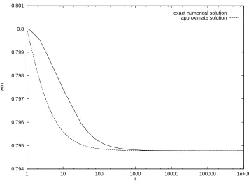
we have a regular event horizon. We now have a hairy black hole metric, caused by the coupling of the geometry to the SU(∞) Yang-Mills field. In figure 1 we compare the approximate solution (51), with the exact numerical solution in the SU(2) case, where
f has the form (40). We use parameters Λ = −100 and w(rh) = 0.8. It can be seen
that the approximate solution converges a little too quickly, but otherwise has the same qualitative features as the exact solution in this case. The approximation would become better if we used more terms in the expansion (45), or if |Λ| was larger.
an infinite number of parameters is required in order to describe it. As mentioned above, the gauge field requires an infinite number of constants for it to be specified in this approximation, since two arbitrary functions of ξ are involved. Each subsequent term in the expansion in ǫ will introduce a further function of ξ into the gauge field, and hence a further infinite number of quantities. Suppose, however, that we wish to fix the behaviour of the gauge field at, say, the event horizon (this was the procedure used to fix the constants in order to obtain figure 1, and is more convenient computationally than fixing quantities at infinity). This would require an infinite number of quantities to specify, say f0(ξ). The subsequent functions of ξ would be fixed by requiring that
fi(r, ξ) = 0 at r=rh for i >0, for example this would mean that
F2(ξ) =
2π√3F1(ξ)
r2
h
. (56)
The result, either way, is that an infinite number of parameters are needed to specify the gauge field function. Next we turn to the metric functions. These do not depend on ξ, but do contain constants constructed from the gauge field function by integrating over ξ. Each term in the perturbation expansion of the metric functions involves at least one new constant constructed from the gauge field function (which cannot be determined from previous constants) as well as a constant of integration. The constants of integration can easily be fixed by the boundary conditions on the metric i.e. by setting δi →0 asr → ∞
for i >0 so that the geometry has the correct behaviour at infinity, and setting qi = 0 at
r = rh for i ≥ 2 so that there is a regular event horizon at r =rh. However, an infinite
number of different constants, coming from the gauge field function, will be required if we are to specify the metric to all orders inǫ. Thus, while it appears that we only need a finite number of constants to construct the metric to each order in perturbation theory, the exact metric will need an infinite number of constants, so that we do have infinite amounts of hair.
3.3
Solutions with a small gauge field
(RN AdS) space, with chargeQ= 1. Therefore in this section we are in effect considering perturbations about this configuration.
Let ε be a small parameter such that ε ≪ 1 and |f(r, ξ)| ≤ ε for all r, so that the magnitude of the gauge field is uniformly bounded and is close to zero. The parameter ε
determines the magnitude of the gauge field (no matter what the size of the cosmological constant Λ) and should not be confused with ǫ = 1/Λ of the previous section where
|Λ| ≫1. This condition of uniform boundedness is rather strong, as we shall see shortly, and the negative cosmological constant is crucial if this condition is to be met. We then consider the following asymptotic expansions of the field variables as ε→0:
f(r, ξ) = εhf0(r, ξ) +εf1(r, ξ) +ε2f2(r, ξ) +. . .i m(r) = m0(r) +εm1(r) +ε2m2(r) +. . .
δ(r) = εδ1(r) +ε2δ2(r) +. . . . (57)
These expansions are inserted into the field equations (29,37,38), as a consequence of which f1, m1 and δ1 all vanish identically. In addition, we have, to lowest order, the RN AdS geometry, so that
m0(r) = 1 2rh
+ rh 2 −
Λr3
h
6 − 1
2r. (58)
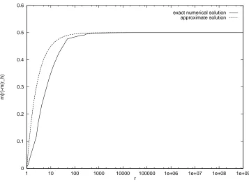
In fact this is a good approximation to the exact metric functionm, as can be seen from figure 2, where we compare (58) with the exact numerical solution for theSU(2) case with Λ =−0.001 andw(rh) = 0.1. Again, the approximate solution has the correct qualitative
features and just converges a little too quickly.
The Yang-Mills equation, to lowest order, tells us that theξdependence off0is arbitrary (subject to (39)), but itsr dependence is governed by the following differential equation:
r2 1− 2m0
r −
Λr2 3
!
∂2f 0
∂r2 + 2m0− 2Λr3
3 −
1
r
!
∂f0
∂r +f0 = 0. (59)
This is exactly the same equation satisfied by very small SU(2) gauge fields, and in this case we can see that the gauge field effectively becomes an infinite number of SU(2) degrees of freedom. The interaction between the degrees of freedom does not come into play in this approximation because the gauge field is very small (and so we have ignored terms involving f2).
which the gauge field is uniformly bounded and arbitrarily small. This is very different to the situation when Λ = 0, when w→ ±1 as r → ∞, so that any gauge field which is very small close to the event horizon, must become order unity at infinity. In this case our expansion in terms of εis not uniformly valid. For Λ>0, it is possible to have gauge fields which are uniformly arbitrarily small, however, in that case, the set of parameters
w(rh) which lead to regular black hole solutions consists of discrete points [18]. When the
cosmological constant is negative, we have regular black hole solutions for a continuous interval of values ofw(rh) containing zero, although the size of this interval shrinks to zero
as Λ→0− [12]. Therefore, for any negative cosmological constant (no matter how small
or large), we can specify any sufficiently small function f(ξ) satisfying the ansatz (39) to be the gauge field function at the event horizon, and then we have infinite gauge field hair which remains arbitrarily small at all distances away from the black hole horizon, including up to the boundary of AdS. It is for this reason that we view the Λ → 0−
model as a “regulator” model for SU(∞)-hair on asymptotically flat space-times with zero-cosmological constant. A zero-cosmological-constant situation might be desirable from both theoretical and phenomenological points of view, e.g. it may be the result of a space-time symmetry like supersymmetry. Notably, in the two-dimensional stringy analogue of the W-hair [4], the ground-state energy of the two-dimensional string has been preserved under the action of the W∞ symmetries [19] and this could be viewed as
the analogue of a zero-cosmological constant situation.
4
Conclusions
In this work we have formulated the field equations for spherically-symmetric EYM black holes in SU(∞) gauge theory. Their study was motivated by some considerations in string theory, the holographic principle and the so-called AdS/CFT correspondence. We have solved these equations both numerically and analytically in some cases. The intro-duction of a negative cosmological constant (no matter how small) proved extremely useful in simplifying the equations by means of appropriate perturbative expansions. Specifi-cally, we have obtained solutions for the cases: (i) Λ <0 with |Λ| ≫ 1, and finite gauge fields, and (ii) Λ<0 arbitrary, and infinitesimally small gauge fields. The latter case ex-hibits holographic properties of the gauge-field hair and may be relevant for issues related to information loss.
quan-tify entropy production during an evaporation process for the case of an SU(2) EYM black hole, coupled to scalar matter [21]. This can be done by identifying the target-space temporal evolution parameter, ‘time’ t, with the logarithm of the brick-wall scale, interpreted as a Renormalization-Group scale that regularizes ultraviolet (short-distance) infinities in the coupled matter/black hole system. One then concentrates on the logarith-mic divergences in the expression for the entropy of the scalar field. Such divergences are extra divergences that cannot be absorbed in a standard renormalization of Newton’s or other field-theory coupling constants (which for instance yield a regularized Bekenstein-Hawking area law [21]). In that sense, such terms have been interpreted in [20] as entropy production.
If the holographic properties of the SU(N → ∞) EYM AdS background were to be extended to the quantum case, such logarithmic divergences should have been suppressed by inverse powers ofN → ∞. However, it can be easily seen that this is not the case for a minimally-coupled scalar field neutral under the gauge symmetry. Indeed, the geometries we consider are small perturbations near RN AdS black-hole space times, and therefore the entropy of a scalar field interacting with this geometry is very nearly the same as the RN AdS case, which is known to be non-trivial [22]. However, the case of a scalar field coupled to the gauge degrees of freedom, which exhibit the holographic properties, may completely change the picture. We hope to return to this issue in a future work. Nevertheless, we believe that the results presented in this work are of sufficient interest to motivate further studies in the above direction.
Acknowledgements
References
[1] R. Bartnik and J. McKinnon, Phys. Rev. Lett. 61 (1988) 141.
[2] P. Bizon, Phys. Rev. Lett. 64 (1990) 2844.
[3] J.H. Schwarz, Target Space Duality and the Curse of the Wormhole, Proc. Int. Conf. on High Energy Physics: Beyond the Standard Model-II, Norman, Oklahoma, Novem-ber 1-3, 1990 (eds. K. A. Milton, R. Kantowski and M. A. Samuel, World Scientific, 1991) p. 384;
S. Kalara and D.V. Nanopoulos, Phys. Lett. B267 (1991) 343.
L. Susskind, Phys. Rev. D49 (1994) 6606; ibid. D52 (1995) 6997.
[4] J. Ellis, N.E. Mavromatos and D.V. Nanopoulos, Phys. Lett. B272 (1991) 261.
[5] I. Bakas, Phys. Lett. B228 (1989) 57; Comm. Math. Phys. 134 (1990) 487;
I. Bakas and E. Kiritsis, Int. J. Mod. Phys. A6 (1991) 2871, and references therein.
[6] L. Krauss and F. Wilczek, Phys. Rev. Lett. 62 (1986) 380;
S. Coleman, J. Preskill and F. Wilczek, Nucl. Phys. B378 (1992) 175.
[7] E.G. Floratos, J. Iliopoulos and G. Tiktopoulos, Phys. Lett. B217 (1989) 285.
[8] N.E. Mavromatos and E. Winstanley, J. Math. Phys. 39 (1998) 4849.
[9] G. ‘t Hooft, in Salamfest 1993, p. 284, gr-qc/9310026;
L. Susskind, J. Math. Phys. 36 (1995) 6377.
[10] J. Maldacena, Adv. Theor. Math. Phys. 2 (1998) 231.
[11] E. Witten, Adv. Theor. Math. Phys. 2 (1998) 253.
[12] E. Winstanley, Class. Quant. Grav. 16 (1999) 1963.
[13] H.P. K¨unzle, Class. Quant. Grav. 8 (1991) 2283.
[14] B. De Wit, J. Hoppe and H. Nicolai, Nucl. Phys. B305 (1988) 545.
[15] O. Brodbeck and N. Straumann, J. Math. Phys. 37 (1996) 1414.
[16] S.W. Hawking and D.N. Page, Comm. Math. Phys. 87 (1983) 577.
[18] M.S. Volkov, N. Straumann, G. Lavrelashvili, M. Heusler and O. Brodbeck, Phys. Rev. D54 (1996) 7243.
[19] E. Witten, Nucl. Phys. B373 (1992) 187.
[20] J. Ellis, N.E. Mavromatos, D.V. Nanopoulos and E. Winstanley, Mod. Phys. Lett. A12 (1997) 243.
[21] N.E. Mavromatos and E. Winstanley, Phys. Rev. D53 (1996) 3190.
0.794 0.795 0.796 0.797 0.798 0.799 0.8 0.801
1 10 100 1000 10000 100000 1e+06
w(r)
r
[image:23.612.134.490.207.472.2]exact numerical solution approximate solution
Figure 1: Comparison of the exact, numerical solution for the gauge field with gauge groupSU(2), where Λ =−100 andwh = 0.8 and the approximate solution given by (51).
0 0.1 0.2 0.3 0.4 0.5 0.6
1 10 100 1000 10000 100000 1e+06 1e+07 1e+08 1e+09
m(r)-m(r_h)
r
[image:24.612.134.491.201.462.2]exact numerical solution approximate solution
Figure 2: Comparison of the exact, numerical solution for the metric functionm(r)−m(rh)
with gauge group SU(2), where Λ =−0.001 andw(rh) = 0.1 with the RN AdS solution,