A Numerical and Analytical Study of Detonation Diffraction

Detonation Diffraction

Thesis by

Marco Arienti

In Partial Fulfillment of the Requirements for the Degree of

Doctor of Philosophy

California Institute of Technology Pasadena, California

2003

c

Acknowledgements

I would first like to thank my advisor, Joseph Shepherd, whose enthusiasm has been a constant source of inspiration in the long years leading to the preparation of this thesis. This work could be completed only thanks to his insight in all aspects of detonation theory, modeling and experiments.

My education at GALCIT has profited from several discussions with Eric Morano and Patrick Hung, who also provided part of the code I used in my computations. I am indebted to Michael Aivazis and Julian Cummings at the Center for Advanced Computing and Research at Caltech for their assistance in cross-platform compilation, as well as for their attempts to train me to a more rigorous programming discipline. By permitting an easy and unrestricted access to the computational resources of the Center, Michael offered the ideal environment for my research. Professor Manish Parashar at Rutgers University provided the framework for parallel simulations with his software package GrACE, and a kind assistance that was very much appreciated. I would also like to thank several other researchers at GALCIT for their useful insights in fluid mechanics in general and physics of detonations in particular – Eric Schultz, Joanna Austin, Eric Winterberger, Demos Kivotides, Ravi Samtaney and Cristopher Eckett. Suzy Dake’s secretarial talents were appreciated as were the proofreading skills of Melinda Kirk. I also thank Professors Hans Hornung, Dan Meiron, Tim Colonius, and Ron Cohen, for taking the time to read my thesis and for serving on my examining committee.

Finally, and most importantly, I am grateful to my wife, Valeria, for her years of moral support and patience.

Abstract

Contents

Acknowledgements iii

Abstract v

List of Figures x

List of Tables xix

Nomenclature xx

1 Introduction 1

1.1 Detonation wave structure . . . 1

1.2 Detonation diffraction . . . 5

1.2.1 Experimental observations . . . 7

1.2.2 Direct numerical simulations . . . 9

1.3 Thesis outline . . . 10

2 Governing equations 13 2.1 Reactive Euler equations . . . 13

2.2 Reactive Euler equations in intrinsic coordinates . . . 15

2.3 The Lagrangian derivative of temperature . . . 17

2.4 Quasi-steady, quasi-one-dimensional reaction zone . . . 20

2.5 The reaction mechanism . . . 24

3.2 Numerical integration . . . 26

3.2.1 Parallel implementation . . . 28

3.3 Shock and flow gradient tracking . . . 29

3.4 Lagrangian particles . . . 31

3.4.1 Lagrangian particles integration . . . 33

3.5 Computational setup . . . 34

3.5.1 Boundary conditions . . . 34

3.5.2 Initial conditions . . . 36

4 Activation energy studies 39 4.1 Coarse-resolution studies . . . 40

4.1.1 Low activation energy . . . 42

4.1.2 High activation energy . . . 43

4.1.3 Intermediate activation energy . . . 44

4.2 High-resolution studies . . . 45

4.2.1 Case θCJ = 1 . . . 45

4.2.1.1 Particle analysis . . . 54

4.2.2 Case θCJ = 4.15 . . . 56

4.2.2.1 Particle analysis . . . 59

4.2.3 Case θCJ = 3.5 . . . 65

4.2.3.1 Particle analysis . . . 73

4.3 Conclusions: a failure model for diffraction . . . 80

5 Wave front models 83 5.1 Skews’ construction for diffracting detonations . . . 83

5.2 Detonation asymptotics . . . 85

5.3 Reduction to blast equation . . . 90

5.4 Whitham shock dynamics . . . 93

6 Transverse wave formation 102

6.1 Computational setting . . . 103

6.2 Non-reactive reference case . . . 103

6.3 Linear acoustic theory . . . 104

6.4 Comparison of different reaction models . . . 108

6.5 Growth of transverse waves . . . 114

7 Summary 118

Bibliography 122

A Convergent evaluation of curvature 129

B Effect of corner radius of curvature 133

List of Figures

1.1 Sooted aluminum sheet. From Kaneshige (1999). . . 2

1.2 Temperature and pressure profile for a ZND wave as a function of the distance behind the shock. . . 3

1.3 Mole fraction profile for a ZND wave. . . 4

1.4 Sonic parameter for a ZND wave. . . 4

1.5 Schematic of a diffracting shock (Skews’ construction). . . 6

1.6 Laser shadowgraph of super-critical diffraction of 100 kPa C₂H₂+1/2 O₂. From Schultz (2000). . . 7

1.7 Laser shadowgraph of sub-critical diffraction of 70 kPa H₂ + 1/2 O₂. From Schultz (2000). . . 8

1.8 Laser shadowgraph of near-critical diffraction 100 kPa H₂+1/2 O₂. From Schultz (2000). . . 9

1.9 Detonation diffraction around a corner. –·–· denotes the plane of symmetry of the channel, H the channel half-width. . . 11

2.1 Intrinsic coordinatesξ and η for an arbitrary front, (a), and specialized to a cylindrical front, (b). . . 15

2.2 Example ofDn(κ) relation for single-step reaction mechanism,Ta= 4.15 times the post-shock temperature. The curvature is normalized by the reference half-reaction length. . . 22

3.2 Comparison of the residual (left-hand side of Equation (2.18) minus right-hand side). Solid line: unsteady term computed via Equation (2.19). Dashed line: unsteady term computed via Equation (3.11). . . 32 3.3 Boundary conditions. . . 34 3.4 Pressure, density, temperature, progress variable and particle velocity

as a function of the distance from the shock η in a ZND profile com-puted for a single-step reaction model with zero activation energy. The particle velocity is divided by the Chapman-Jouguet detonation speed

DCJ, whereas all the other variables are normalized by the corresponding post-shock (von Neumann) values. . . 37 3.5 ZND pressure profiles versus distance from the shock. The curves are

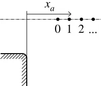
computed from the values of θCJ and k listed in Table 3.1. The line passing through the square symbols corresponds to zero activation en-ergy. . . 37 4.1 Distance from the corner, measured along the channel axis of symmetry,

xa, and along the corner wall, yw. . . 40 4.2 Detonation velocity at the axis, Da, as a function of the distance

mea-sured from the vertex, xa. The labels are values of the non-dimensional activation energy θCJ, varying from 0 to 4.15. . . 41 4.3 Detonation velocity at the corner wall, Dw, as a function of the distance

from the vertex, yw. The labels are values of the normalized activation energy θCJ, varying from 0 to 4.15. . . 42 4.4 Detonation velocity - curvature (Dn−κ) diagram at the axis of symmetry

of the channel. The labels are values of the normalized activation energy

θCJ, varying from 0 to 4.15. . . 44 4.5 Numerical schlieren images for the case θCJ = 1. (a) t = 13.83; (b)

4.6 Pressure profile (a) and sonic parameter (b) for 5 data sets extracted at

t = 35.79. Slice 1 and 5 are extracted along the axis of symmetry and the corner wall, respectively. The remaining data are taken in the shock normal direction and are evenly spaced along the detonation front. . . 47 4.7 Numerical schlieren image, (a), and contours of u2/c2−1, (b). The red

line is the 0.95 reaction locus. In (b), the contours have values ranging from −1 to 8, with spacing equal to 0.25. Dashed lines correspond to

u ≤ c and solid lines to u > c. Every dashed contour that is adjacent to a solid contour represents a sonic line in the laboratory frame. The plots are a close up of the frame at t = 28.47 in Fig. 4.5, computed for

θCJ = 1. . . 49 4.8 Contours of pressure (left), and numerical schlieren images of density

(right) at time t = 8.5 (a), and t = 13.83 (b), computed for θCJ = 1. The pressure increment of the contours is 0.8334 up to a cutoff value of 50 times the ambient pressure. The reference segment (bottom right corner of the contour plots) measures ∆₁/2. . . 51 4.9 Sequence of transverse waves along the detonation front at time t =

35.79 for θCJ = 1. Frame (a): schlieren image. The solid line is the locus of 95% reaction completion. The reference segment (bottom right corner) measures 10 ∆₁/2. Frame (b): contours of c2 −(7.010−ux)2− (7.010−uy)2 from -20 to 15 with spacing equal to 1. . . 53 4.10 Location of injected particles. . . 54 4.11 Particle paths for 10 sample particles injected along the vertical corner

4.13 Terms in the reaction zone temperature Equation (2.18) along the same particle paths as in Fig. 4.11 for the case θCJ = 1. The particles are injected along the vertical wall of the corner. · · · ·Lagrangian temper-ature; –·–· heat release; – – – curvature; — — transverse divergence; –··–·· unsteadiness. The solid line is the difference between the left-hand side and the right-left-hand side in Equation (2.18), as computed from the above terms. (a) Particle 1; (b) Particle 7. . . 56 4.14 Numerical schlieren images for the case θCJ = 4.15. (a) t = 22.24; (b)

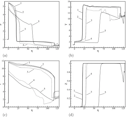
t = 28.43; (c)t = 34.63; (d)t= 40.83. (e)t= 47.02; (f) t= 53.22. . . 57 4.15 Density (a), temperature (b), pressure (c) and progress variable (d)

profiles for 5 different data set extracted at t= 53.22. . . 58 4.16 Numerical schlieren image, (a), and contours of u2/c2−1, (b). The red

line is the 0.95 reaction locus. In (b), the contours have values ranging from −1 to 8, with spacing equal to 0.25. Dashed lines correspond to

u≤cand solid lines tou > c. Every dashed contour that is adjacent to a solid contour is a sonic line in the laboratory frame. The plots are a close up of the frame at t= 28.43 in Fig. 4.14, computed forθCJ = 4.15. 60 4.17 Space-time diagram for failing detonation (θCJ = 4.15). Shock (solid

line); sonic loci (dotted line); 0.05 and 0.95 reaction loci (broken line). 61 4.18 Location of injected particles. . . 61 4.19 Particle paths for ten sample particles. Shock (thick solid line); particle

4.21 Terms in the reaction zone temperature Equation (2.18) along the same particle paths as in Fig. 4.19 for θCJ = 4.15. The particles are in-jected on the channel axis of symmetry. · · · · Lagrangian tempera-ture; –·–· heat release; – – – curvature; — — transverse divergence; –··–·· unsteadiness. The solid line is the difference between the left-hand side and the right-left-hand side in Equation (2.18), as computed from the above terms. (a) Particle 1; (b) Particle 3; (c) Particle 5; (d) Particle 10. . . 64 4.22 Numerical schlieren images for the case θCJ = 3.5. (a) t = 10.17; (b)

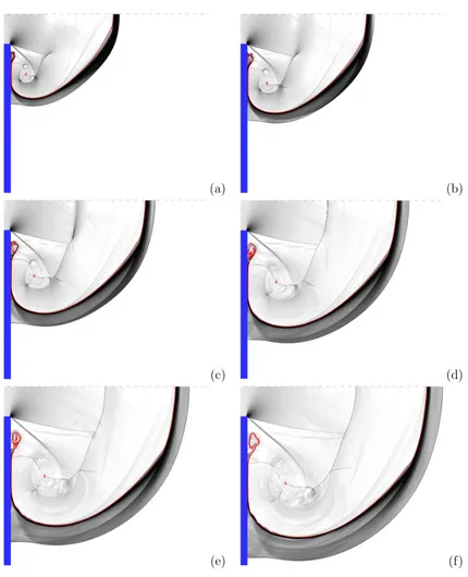
t = 13.83; (c) t = 17.49; (d) t = 21.15. (e) t = 22.98; (f) t= 24.81; (g)

t = 26.64; (h)t= 28.47. . . 66 4.23 Numerical schlieren images for the case θCJ = 3.5. (i) t = 32.13; (l)

t = 35.79; (m)t= 39.45; (n) t= 43.11. (o) t= 44.94; (p) t= 46.77. . 67 4.24 Pressure contours (left) and numerical schlieren images (right) for the

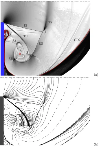
case θCJ = 3.5 at times t = 9.255 (a); 11.08 (b); 12.91 (c); 15.66 (d); 17.49 (e). Each plot measures 86.7 half-reaction lengths in width. . . . 68 4.25 Structure of transverse wave, contours of pressure, (a), and numerical

schlieren images of density, (b). The solid line in (b) is the 0.95 reaction locus. In (a), contour lines are spaced by the non-dimensional value 2.083. A cutoff value of 250 is used (the local maximum value is 445), to mark the pressure peak position behind the kink. The segment at the bottom left indicates the length of ∆₁/2 in the plot scale. The two images are a close up of a frame att = 30.30 computed for θCJ = 3.5. 70 4.26 Numerical schlieren images for the case θCJ = 3.5. Each frame is a close

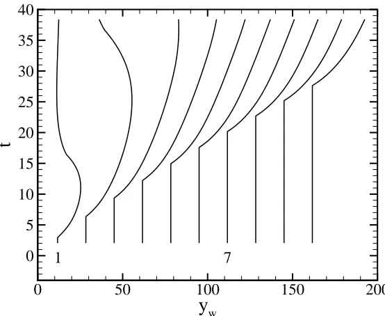
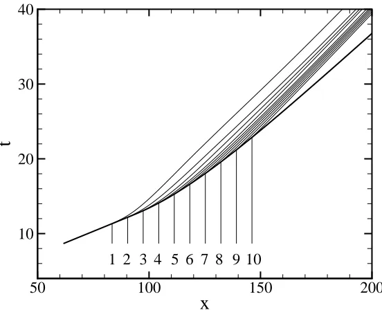
4.27 Space-time diagram for the leading shock and the 0.05 and 0.95 reaction loci along the axis of symmetry. Solid line leading shock; – – – progress variable 0.05; · · · · progress variable 0.95. . . 74 4.28 Space-time diagram for the leading shock and the 0.05 and 0.95 reaction

loci along the wall. Solid line leading shock; – – – progress variable 0.05;

· · · · progress variable 0.95. . . 75 4.29 Particle paths for 21 sample particles injected along the channel axis

(Fig. 4.18) forθCJ = 3.5. The labels 1, 10, 16, 21 indicate particles that are analyzed in terms of numerical dominant balance. . . 76 4.30 Particle paths for 20 sample particles injected along the vertical corner

wall (Fig. 4.10) forθCJ = 3.5. The labels 1 and 10 indicate the particles that are analyzed in terms of numerical dominant balance. . . 77 4.31 Temperature profiles along the particle paths displayed in Fig. 4.29. . . 77 4.32 Temperature profiles along particles paths displayed in Fig. 4.30. . . . 78 4.33 Terms in the reaction zone temperature Equation (2.18) along the same

particle paths as in Fig. 4.29 for the case θCJ = 3.5. The particles are injected along the axis of symmetry. · · · · Lagrangian tempera-ture; –·–· heat release; – – – curvature; — — transverse divergence; –··–·· unsteadiness. The solid line is the difference between the left-hand side and the right-left-hand side in Equation (2.18), as computed from the above terms. (a) Particle 1; (b) Particle 10.; (c) Particle 16; (d) Par-ticle 21. . . 79 4.34 Terms in the reaction zone temperature Equation (2.18) along the same

5.1 Schematic of a diffracting shock (Skews’ construction). . . 84 5.2 Sound speed, relative particle velocity, square root of the sonic

param-eter, frame (a), and disturbance angle plotted vs. the progress variable

Z, frame (b). . . 85 5.3 Dn–κ diagram for θCJ = 1. —— evaluated along the channel axis of

symmetry and the corner wall from numerical simulation; – – – com-puted for quasi-steady, quasi-one-dimensional reaction zone. . . 86 5.4 Dn–κdiagram along the channel axis of symmetry forθCJ = 3.5. ——

eval-uated along the channel axis of symmetry from numerical simulation; – – – computed for quasi-steady, quasi-one-dimensional reaction zone. 87 5.5 Dn–κ diagram along the channel axis of symmetry for θCJ = 4.15.

—— evaluated along the channel axis of symmetry from numerical sim-ulation; – – – computed for quasi-steady, quasi-one-dimensional reaction zone. . . 88 5.6 Shock deceleration as a function of the distance from the corner vertex,

parametrized by θCJ. . . 91 5.7 Detonation diffraction around a corner. –·–· denotes the axis of

sym-metry of the channel . . . 97 6.1 Detonation running over an obstacle. . . 102 6.2 Non-reactive shock over an obstacle. . . 104 6.3 Detail of shock interaction for the non-reactive case. (a) schlieren image;

(b) pressure diagrams The four horizontal lines (numbered 1, top, to 4, bottom) in (a) mark where data have been extracted to draw the pressure plots. . . 105 6.4 Geometry of the wavefront. . . 106 6.5 Threshold value of normalized activation energy for amplification plotted

6.7 Computational cases A and B, detail of the solution (schlieren image), left, and pressure diagram, right. The four horizontal lines (numbered 1, top, to 4, bottom) mark where data have been extracted to draw the pressure plots. The dashed line on the left is the locus of 50% reaction completion locus. Frames (a) and (b); order 1 reaction. Frames (c) and (d); order 2 reaction. . . 110 6.8 Computational cases C and D, detail of the solution (schlieren image),

left, and pressure diagram, right. The four horizontal lines (numbered 1, top, to 4, bottom) mark where data have been extracted to draw the pressure plots. The dashed line on the left is the locus of 50% reaction completion locus. Frames (a) and (b); order 1 reaction. Frames (c) and (d); order 2 reaction. . . 112 6.9 Frames (a) to (c): contours ofω, Equation (6.13), for cases A, B, C. The

contours start at the value -20 and are spaced by 0.50. The plot scale is the same used for the schlieren images in Fig. 6.7 and Fig. 6.8. Frames (d) to (f): plot of s for cases A, B, C along slices taken at the locations shown in the upper diagrams. . . 113 6.10 Space-time diagram of the transverse wave system for pressure (a), and

superposition of the same data showing the growth of wave S2 (b). . . 116 6.11 Pressure peak vs. time for S2 wave. Symbols: peak value of S2 in

the pressure diagrams of Fig. 6.10 (b). Solid line: least-squares fitting, Equation (6.14). . . 116 A.1 Point selection for computing a second-order derivative. Here h= 2. . 130 A.2 Convergence study for the computed maximum value of curvature as a

function of grid refinement. ¥ grid-adaptive spacing; ¨ fixed point; N fixed spacing. . . 131 A.3 Convergence study for the computed maximum value of curvature as a

B.1 Effect of a finite radius of curvature rc on the wall detonation velocity in the vicinity of the corner. . . 134 B.2 Effect of grid refinement at a constant radius of curvature, rc = 1. The

internal box is a close up of the plot, showing the oscillations in the detonation velocity at the wall. . . 134

C.1 Iso-contours of pressure (left), and numerical schlieren images (right) for three different grid resolutions. (a) N₁/2 = 22.5; (b) N1/2 = 11.2; (c)

List of Tables

Nomenclature

SI Units†

Roman characters

A area function

B wave velocity in the surface kinematics wave equation m/s

c frozen sound speed m/s

Cp mixture specific heat at constant pressure J/kg·K

Cv mixture specific heat at constant volume J/kg·K

D detonation velocity m/s

Da detonation velocity along the channel axis of symmetry m/s ˙

Db initial blast decay rate m/s2

Dn normal detonation velocity m/s

Dw detonation velocity along the corner wall m/s

Ea activation energy in Arrhenius reaction rate J

e specific internal energy J/kg

Et total energy per unit volume J/m3

f detonation overdrive

Fx convective flux vector in x direction (various)

Fy convective flux vector in y direction (various)

H channel half-width m

h number of skipped grid point in the evaluation of curvature

K twice the amplification factor in one-dimensional wave equation 1/s

k pre-exponential factor in model reaction rate (various)

l direction cosine of wave normal with respect to x coordinate

M leading shock strength

m characteristic angle in chapter 5 rad

m direction cosine of wave normal with respect to y coordinate

Ms local flow Mach number with respect to the shock front

n exponent in Whitham’s area function

N₁/2 number of grid points per half-reaction zone length

nr order of reaction

PM Peak value of pressure amplitude Pa

P pressure Pa

Q heat of reaction J/kg

r blast radius m

rb initial blast radius m

Rg specific gas constant of mixture J/kg·K

s amplitude of acoustic disturbance

S reaction source term vector (various)

Ta activation temperature of reaction K

tb initial time in blast model s

t time s

u flow velocity in the laboratory frame m/s

uη flow velocity in normal direction m/s

uξ flow velocity in transverse direction m/s

ux flow velocity in x direction m/s

uy flow velocity in y direction m/s

W conservative solution vector (various)

w flow velocity in the shock frame m/s

W mean molar mass of mixture kg/mol

Wk molar mass of species k kg/mol

wη flow velocity in normal direction in intrinsic coordinates m/s

wξ flow velocity in transverse direction in intrinsic coordinates m/s

x laboratory Cartesian coordinate m

y laboratory Cartesian coordinate m

x₀ x coordinate of intrinsic system reference point m

xb obstacle position m

y vector of species mass fractions

yK mass fraction of species K

Z reaction progress variable in one-step reaction

Greek characters

α angle of the disturbance trace with the undiffracted shock normal rad

∆ induction length m

∆₁/2 ZND half-reaction length for CJ detonation m

² height and width of obstacle m

γ ratio of mixture specific heats

η shock based (intrinsic) coordinates m

κ local front curvature 1/m

κa front curvature along the axis of symmetry 1/m

κd front curvature at the reflection of the firstC+ characteristic 1/m

κb initial blast curvature 1/m

Λ wavelength of acoustic disturbances m

λ detonation cell width m

ν coordinate in the normal direction with respect to the acoustic wavefront m

ω sonic parameter m2/s2

φ front normal angle with respect to the axis of reference rad

ϕ level set function m

˙

σ total thermicity 1/s

σK thermicity coefficient of species K

θ ray angle with respect tox

θCJ activation energy normalized by the CJ post-shock temperature

ξ shock based (intrinsic) coordinates m

ΩK production rate of speciesK 1/s

ζ activation energy normalized byT_k

Subscripts

K species index

k plane of parallel propagation with respect to the detonation front

Accents

Chapter 1

Introduction

1.1

Detonation wave structure

Detonations are supersonic combustion waves with a strong leading shock front. The shock wave ignites the reactive material and the exothermic stage of the reactions creates volume expansion that pushes the shock into fresh reactants.

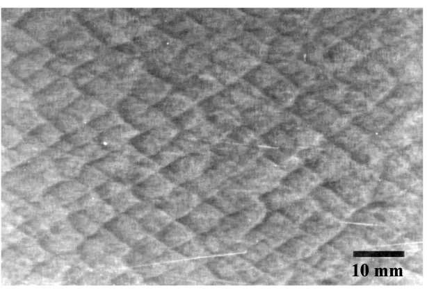
Experiments in reactive mixtures reveal that detonation fronts tend to develop complicated three-dimensional time-dependent structures with interior transverse shock waves (see, for instance, Fickett and Davis 1979). A self-sustaining cellular structure, driven by chemical reactions, is often observed. The cell boundaries are unsteady, decaying transverse waves which propagate at approximately acoustic velocity. They are periodically restored by collision with waves moving in the opposite direction. The variations of pressure and velocity in this structure are sufficient to incise diamond-shaped patterns on sooted plates, see Fig. 1.1 from Kaneshige (1999).

To study this intricate flow field, the simplest, physically relevant mathematical model is provided by the reactive Euler equations of gasdynamics, expressing con-servation of mass, momentum and energy for an inviscid flow. An additional set of equations describes the rate of change of the chemical species as observed by material particles in the flow. Transport effects and dissipative processes are neglected in this model.

Figure 1.1: Sooted aluminum sheet. From Kaneshige (1999).

processes, is followed by a region with a finite rate of reaction. Under these conditions, the reactive Euler equations admit a steady solution in the coordinate system attached to the shock. This solution (the Zel’dovich-von Neumann-Doering, or ZND, wave) propagates at speed D which is a function of the boundary conditions at the end of the reaction zone.

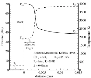
Figure 1.2 shows a representative pressure and temperature profile for a ZND wave computed by Schultz (2000) with a program developed by Shepherd (1986). The program uses the Chemkin II chemical kinetics package and integrates the equa-tions of mass, momentum, energy and species conservation through the reaction zone. (Kee et al. 1989). The species production rates of a stoichiometric C₃H₈–O₂ mix-ture at standard conditions are calculated with the Konnov (1998) detailed reaction mechanism.

distance (cm) P re ss ure (a tm ) Temp er atu re (K )

0 0.005 0.01 0.015

0 10 20 30 40 50 60 70 0 500 1000 1500 2000 2500 3000 3500 4000

Reaction Mechanism: Konnov (1998) C₃H₈+ 5O₂ D_CJ=2361m/s P₁=1atm, T₁=295K

∆= 0.03mm T₁ P₁ P_vN T_vN T_CJ P_CJ ∆ shock induction length

Figure 1.2: Temperature and pressure profile for a ZND wave as a function of the distance behind the shock.

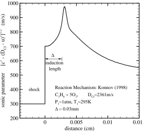
by a rapid rise in temperature, a decrease in pressure, and the formation of the major products of reaction (see Figs 1.2 and 1.3). In this example profile, the sonic parameter c2 −(D−u)2 reaches a peak value at a distance ∆ from the shock and then decreases (Fig. 1.4).

In a Chapman-Jouguet (CJ) wave, the recombination region ultimately passes through a sonic point where the local sound speed equals the particle speed in the ref-erence frame of the shock. The corresponding speed of propagation, DCJ, is the min-imum speed allowed based on thermodynamic arguments (Fickett and Davis 1979). Overdriven detonations (D > DCJ) are also possible when the particle speed u > uCJ at the end of the reaction zone.

distance (cm) M o le F ractio n s (C 3 H8 ,O 2 ,H 2 O, C O2 ) M o le F ractio n (O H )

0 0.005 0.01 0.015

0 0.1 0.2 0.3 0.4 0.5 0.6 0.7 0.8 0.9 1 0 0.05 0.1 0.15 0.2

C₃H₈ O₂ H₂O CO₂ OH

Reaction Mechanism: Konnov (1998) C₃H₈+ 5O₂, D_CJ=2361m/s P₁=1atm, T₁=295K

∆=0.03mm

Figure 1.3: Mole fraction profile for a ZND wave.

distance (cm) so n ic p ar ameter [c 2 -( DCJ -u ) 2 ] 1/ 2 (m/s )

0 0.005 0.01 0.015

200 300 400 500 600 700 800 900 1000

Reaction Mechanism: Konnov (1998) C₃H₈+ 5O₂, D_CJ=2361m/s P₁=1atm, T₁=295K

∆= 0.03mm ∆

shock

induction length

1.2

Detonation diffraction

Detonations diffracting from a planar to a cylindrical (or spherical) geometry through an abrupt area change experience expansion waves that propagate into the partially burnt reactants behind the wavefront.

One of the key features of the diffraction process is the propagation of the sig-nal generated by the expansion waves emanating at the corner. The head of the disturbance intersects the undisturbed detonation, and the propagation speed v of this point can be evaluated with the help of a suitable extension of Skews’ geomet-ric construction for non-reacting diffracting shocks (Skews 1967). In Fig. 1.5, we see that the disturbance is propagating at the local sound speed cwhile being convected downstream at a speed u. The angle α between the disturbance trajectory and the normal of the undiffracted shock, at speed D, can be found with the formula

tanα = v

D =

q

c2−(D−u)2

D .

In the non-reactive cases, the values u and c are determined from the undisturbed post-shock state. In the reactive case, the fact that a finite transverse signal speed is observed in corner-turning experiments with CJ detonations (for instance, Schultz 2000) indicates that these acoustic disturbances must propagate in the reaction zone, between the sonic plane (whereDCJ =uCJ+cCJ by definition) and the leading shock.

The sensitivity of chemical reactions to post-shock conditions is the second key feature in detonation diffraction. Typical reaction rates are of the Arrhenius form. For a single-step reaction model of ordernr, this is

Ω =k ρnr−1(1−Z) e−Ta/ T,

u ∆t

c ∆t head of

corner

signal α

D ∆t undisturbed shock

interaction point

v ∆t

diffracted shock D − u

v c

O

Figure 1.5: Schematic of a diffracting shock (Skews’ construction).

a proportionality parameter setting the length scale of energy release. The sensitivity of the chemical kinetics is expressed in the nonlinear term by the parameter Ta, the activation temperature of the reaction.

At the shock, Z = 0 and T and ρ depend only on the undisturbed flow ahead, at state 0, and on the shock strength, M =D/c₀. For instance, in the limit ofM2 À1, a shock in a perfect gas with specific heat ratio γ generates a jump in temperature and density

Ts

T₀ =

2γ(γ−1) (γ+ 1)2 M

2 ρs

ρ₀ = γ+ 1

γ−1.

Since the shock is weakened by the interaction with expansion waves from the corner,

shock coupled to reaction zone

Figure 1.6: Laser shadowgraph of super-critical diffraction of 100 kPa C₂H₂+ 1/2 O₂. From Schultz (2000).

1.2.1

Experimental observations

decoupled shock reaction

front

Figure 1.7: Laser shadowgraph of sub-critical diffraction of 70 kPa H₂+ 1/2 O₂. From Schultz (2000).

the smallest side of the orifice is larger than 3λ. A recent review of the available detonation diffraction literature can be found in Schultz (2000).

shock

shock and reaction front together reaction front

Figure 1.8: Laser shadowgraph of near-critical diffraction 100 kPa H₂+ 1/2 O₂. From Schultz (2000).

1.2.2

Direct numerical simulations

layer. These cells weakened as soon as they expanded into the lower layer, while new transverse waves formed spontaneously along the shock front, moved toward the rarefaction zone, and ignited unburnt shocked reactants. If an insufficient number of detonation cells (3 or less) was initially contained in the upper layer, the detonation did not propagate into the lower layer. Li and Kailasanath (2000) observed a suc-cessful detonation transmission from a smaller to a larger channel in a stoichiometric ethylene-oxygen mixture when 8 detonation cells were present in the smaller channel. The transmission was unsuccessful in a stoichiometric ethylene-air mixture with only 4 cells.

Pantow et al. (1996) used a two-step MacCormack scheme with FCT to study detonation diffraction of H₂–O₂ mixtures diluted by different amounts of argon or nitrogen. The chemical kinetics were implemented as a two-step parameter model and computations were performed on a time-dependent adaptive grid (no data on grid resolution are reported, but we estimate that at least 45 grid points per detonation cell width were used). As well as illustrating re-ignition after Mach reflection at the confining walls, these simulations show newly formed transverse waves in regions where the detonation front begins to fail.

Simulations with single-step Arrhenius kinetics by Williams et al. (1996) indicate that the generation and interaction of transverse waves are even more intricate in three dimensions. While the grid resolution is quite coarse (only 8 grid points in the reference half-reaction length), Williams’ results show the existence of perpendicular modes which generate vorticity fields more complex than in two dimensions. Vorticity seems to provide a strong coupling mechanism between the perpendicular modes, and is possibly a trigger mechanism for the production of new transverse waves.

1.3

Thesis outline

H

π/2

Figure 1.9: Detonation diffraction around a corner. –·–· denotes the plane of sym-metry of the channel, H the channel half-width.

symmetry, and in Fig. 1.9 we show only the lower half-space of the domain. We will refer to the intersection of the plane of symmetry with the x-y plane as the axis of symmetry of the channel. If we assume an unbounded volume, then the only geometric parameter of the problem is the exit diameter of the tube. In two dimensions, the reference length is the channel half-width, H. Dimensional analysis for the single-step reaction model in the Arrhenius form leads to the following dependence for the critical channel half-width,

Hc

∆₁/2 =g

µ

Q RgT0

, γp, γr, f,

Ta

T₀, n

¶

, (1.1)

where Qis the heat of reaction, γr and γp are the reactant and product specific heat ratios, andf =D/DCJ is the overdrive of the detonation in the channel. The reaction characteristic length∆₁/2is defined as the distance, in the reference CJ wave, between the shock (Z = 0) and the point where Z = 1/2. Our study is further specialized by setting f = 1, γp =γr, and nr= 2.

The concept of shock decoupling from the reaction zone is the simplest idea used to explain the behavior of a diffracting detonation front. Chapter 2 is devoted to the extension to an arbitrary wavefront of the equation framework used in the study of direct initiation of spherically symmetric detonations (Eckett et al. 2000). The numerical implementation of the equations of fluid motion, and the algorithms used for flow diagnostics, are described in Chapter 3.

describes the temperature rate of change of a fluid element. Conveniently simplified, this equation provides the starting point for a critical diffraction model. We examine the mechanism of spontaneous generation of transverse waves due to reflection of the unsteady rarefaction front. This mechanism is related to the sensitivity of the reac-tion rate to temperature, and it is investigated in the form of a parametric study for the activation energy.

In Chapter 5, we review the applicability of existing shock dynamics models to the corner-turning problem. Numerical results from the parametric study are compared with predictions from these theories. The objective is to find a formula for shock decay at the centerline when the detonation front is close to local failure. This formula is then used in the simplified temperature rate of change equation to give a relation between critical diameter and activation energy.

Chapter 6 is devoted to the study of a result that emerged from the computation of fully coupled diffracting detonations: the spontaneous formation of transverse waves along the wavefront. We consider planar CJ detonations, with nr = 1 and nr = 2, moving in a channel over a small obstacle, to study how acoustic waves propagate within the reaction zone. Depending on the reaction kinetics, we show that such waves may be amplified due to feedback between the chemical reaction and fluid motion (Strehlow and Fernandes 1965). The amplification can lead to shock steepening and formation of transverse detonation waves.

Chapter 2

Governing equations

2.1

Reactive Euler equations

Ignoring viscosity, heat transfer, diffusion, radiation and body forces, the governing equations for a compressible reacting flow are the reactive Euler equations (see, for instance, Fickett and Davis 1979). In a fixed Cartesian reference frame, the two-dimensional, reactive Euler equations are given by

Dρ

Dt +ρ ∂ux

∂x +ρ ∂uy

∂y = 0, (2.1a)

Dux Dt +

1

ρ ∂P

∂x = 0, (2.1b)

Duy Dt +

1

ρ ∂P

∂y = 0, (2.1c)

De

Dt − P ρ2

Dρ

Dt = 0, (2.1d)

DyK

Dt =ΩK, (2.1e)

derivative of a variable

D Dt =

∂ ∂t+ux

∂ ∂x +uy

∂

∂y. (2.2)

If we take theeto be a function ofP,ρ, and the mass fraction arrayy={yK, K = 1, . . . , N}, then

De

Dt = ∂e ∂P ¯¯ ¯¯ ρ,y DP

Dt + ∂e ∂v ¯¯ ¯¯ P,y Dv

Dt +

X K ∂e ∂yK ¯¯ ¯¯

P, ρ, yJ₆₌K DyK

Dt . (2.3)

From this expression and Equation (2.1d), we obtain the adiabatic change equation,

DP

Dt =c

2Dρ Dt +ρc

2 X K

σKΩK. (2.4)

In Equation (2.4), cis the constant composition, or frozen, sound speed,

c2 =

P + ∂e

∂v

¯¯ ¯¯

P,y

ρ2 ∂e ∂P

¯¯ ¯¯

ρ,y

, (2.5)

and σK is the thermicity coefficient of species K,

σK = 1 ρc2 ∂P ∂yK ¯¯ ¯¯

e, ρ, yJ₆₌K

= − 1

ρc2 ∂e ∂yK

¯¯ ¯¯

P, ρ, yJ₆₌K

∂e ∂P ¯¯ ¯¯ ρ,y . (2.6)

In this work, we will find it useful to replace the energy equation (2.1d) with the adi-abatic change equation. The sum of the thermicity coefficients σK in Equation (2.4) expresses the total pressure change due to chemical reaction at constant volume. This last term is called the thermicity product ˙σ,

˙

σ =X

K

ξ

η η

η φ

(x , y )_{0 0}

η1

η2 Dn

x y

x y

ξ

(x , y )_{0 0}

η

η₁ η₂ η

φ Dn

(a) (b)

Figure 2.1: Intrinsic coordinates ξ and η for an arbitrary front, (a), and specialized to a cylindrical front, (b).

2.2

Reactive Euler equations in intrinsic coordinates

The analysis of the reactive Euler equations can be carried out by using intrinsic, shock-based coordinates as independent variables. While more cumbersome than the Cartesian description of the previous section, this approach allows for a direct comparison with the system of equations that can be derived for cylindrical symmetry. In this way, the effect of shock front curvature can be more easily examined. As we will show, the formulation in intrinsic coordinates simplifies noticeably along an axis of symmetry of the flow. In this case, only one additional term, due to the transverse flow divergence behind the leading shock, is formed in comparison to the cylindrical case (Eckett et al. 2000).

In intrinsic coordinates (Fig. 2.1), the variable ξ measures the arc length of the leading shock from a reference point (x₀, y₀). Along the shock, the second coordinate

η is constant and is equal to zero. Lines of constant η are the loci of points with the same distance from the shock. The angle φ, formed by the normal to the front with respect to a reference axis, is a dependent variable,φ(ξ, t). The two-dimensional curvature of the front,κ, is by definitionκ= (∂φ/∂ξ)_{η, t}. Dnis the detonation velocity normal to the front.

η=R−r, and we find the trivial result κ= 1/R.

Conservation of mass, momentum and total energy can be written in intrinsic coordinates as (Bdzil and Aslam 2000),

L(ρ) + [(Dn−uη)ρ],η+ρ

uηκ+uξ,ξ

1−η κ = 0, (2.8a)

L(uη) + (Dn−uη)uη,η =

P,η

ρ −

uξ(Dn,ξ−uξκ)

1−η κ , (2.8b)

L(uξ) + (Dn−uη)uξ,η =−

P,ξ+ρuη(uξκ−Dn,ξ)

ρ(1−η κ) , (2.8c)

L(e) + (Dn−uη)e,η =

P

ρ2[L(ρ) + (Dn−uη)ρη], (2.8d)

where we use the notation , ξ and , η to indicate a partial derivative with respect to

ξ and η, in this order. The operator

L= ∂

∂t ¯¯ ¯¯ ξ, η + µ

B+ uξ−ηDn,ξ 1−η κ

¶ ∂ ∂ξ ¯¯ ¯¯ t, η , (2.9)

and uη, uξ are the particle velocity components in the shock normal and transverse direction. Where intrinsic coordinates can be used, the set (2.8) is completely equiv-alent to the set (2.1)(a) to (d). Note, however, that the partial time derivatives in the Cartesian and intrinsic system differ,

∂ ∂t ¯¯ ¯¯ ξ,η 6 = ∂ ∂t ¯¯ ¯¯ x,y , (2.10)

since the intrinsic reference system is time varying.

In Equation (2.9),B is the wave velocity in the surface kinematics equation (Bdzil and Stewart 1989)

φ,t+B φ,ξ =−Dn,ξ. (2.11)

can be expressed as a function of curvature and normal shock velocity,

B =

Z ξ

0

φ,ξDndξ+B0(t). (2.12)

The term B₀(t) accounts for a finite angle between the shock normal and the axis of reference. By inspection of the equations above, the Lagrangian derivative of a variable is expressed as

D/Dt=L+ (Dn−uη) ∂/∂η. (2.13)

2.3

The Lagrangian derivative of temperature

The simplest concept of detonation failure is a decoupling of the reaction zone from the shock front, or equivalently, the failure of particles to rapidly undergo reaction after they cross the shock. Since most of the reaction rate laws are strongly temperature dependent, we now focus our attention to the Lagrangian derivative of temperature, DT /Dt. To do so, we need to close the set of reactive Euler equations with a thermal equation of state. For simplicity, we consider a mixture of perfect gases

P =ρ RgT, (2.14)

where Rg is the mixture gas constant

Rg =

R

W =R

X _yK

WK

. (2.15)

R is the universal gas constant, W the mixture molar mass and WK is the molar mass of species K. The frozen sound speed is

c=

µ

γ P ρ

¶₁/2

, (2.16)

To analyze the relative importance of the wavefront local flow features, it is con-venient to express DT /Dtin the intrinsic coordinate system described in the previous section. By taking the Lagrangian derivative of Equation (2.14), and using the adi-abatic change equation (2.4) together with the mass and momentum equations in (2.8), we find the temperature reaction zone structure equation

µ

1− w 2 η c2 ¶ Cp DT

Dt = (2.17)

= 1

γ−1

¡

c2−γ w2_η¢ σ˙ heat release +w2_η κ(Dn−wη)

1−η κ curvature

+wη (Dn−wη),t+

P,t

ρ unsteadiness

+w2_η wξ,ξ

1−η κ divergence

−wη

w_ξ2κ

1−η κ centripetal

+ wξ

1−η κ (−wηwη,ξ+ P,ξ

ρ ) N1

+B (wη(Dn−wη),ξ+

P,ξ

ρ ) N2

− ηDn,ξ

1−η κ (wη(Dn−wη),ξ + P,ξ

ρ ) N3

+wξwη

2Dn,ξ

1−η κ N4

withwη =Dn−uη and wξ =uξ. Cp is the mixture specific heat at constant pressure,

Cp =Rgγ/(γ−1). The left-hand side of Equation (2.17) has the dimension of energy density per unit time. The right-hand side has terms depending from the thermicity product, shock curvature, partial time derivatives of the flow, transverse divergence

wξ,ξ, and also a term that has the appearance of work associated with centripetal motion. The remaining terms in (2.17) are more difficult to interpret, and are simply labeled N1 to N4.

to as “unsteady terms” or “unsteadiness” for the fluid particle. For a decelerating wave such as in a detonation diffraction, the unsteady terms are negative. Thus, the reaction may quench if the wave is decelerating too rapidly. When the wavefront is convex-upstream, the curvature term is positive, and so it cannot possibly quench the reaction without the additional presence of unsteadiness.

If the axis of reference is also an axis of symmetry for the flow field, several terms disappear atξ = 0. The transverse derivatives vanish, with the exception ofwξ,ξ, and we obtain

µ

1− w 2 η

c2

¶

Cp DT

Dt =

1

γ −1

¡

c2−γ w_η2¢ σ˙ heat release (2.18) +w_η2 κs(Ds−wη)

1−η κs

curvature +wη (Ds−wη),t+

P,t

ρ unsteadiness

+w_η2 wξ,ξ

1−η κs

divergence

In Equation (2.18),κs(t) andDs(t) are the front curvature and shock speed evaluated on the axis of symmetry. The result is the same found for a cylindrically symmetric flow with the addition of a transverse divergence term. This term is always positive since wξ is antisymmetric and no mass flux is allowed at the axis of symmetry.

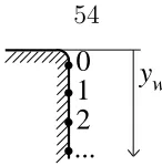
The relative size and behavior of the terms in the temperature reaction zone structure equation will be examined numerically by following the path of massless particles injected into the flow. We will refer to these particles as Lagrangian. While this procedure can be applied to a general flow, the analysis can be restricted to regions where the shock is normal and the flow is parallel to the reference axis, so that Equation (2.18) can be used. Such regions are the channel axis of symmetry and the corner wall, i.e., the two boundary regions of a diffracting wavefront. The goal is to identify the dominant balance in a Lagrangian particle close to ignition failure and to find any simplifying assumption regarding the behavior of terms in (2.18).

conditions of symmetry,

wη (Ds−wη),t+

P,t

ρ =

1

ρ

µ

DP

Dt −w

2 Dρ Dt

¶

+w2_η κs(Ds−wη)

1−η κs

+w_η2 wξ,ξ

1−η κs

. (2.19)

This formula is useful in the numerical evaluation of the unsteady terms of Equation (2.18), since it provides an alternative to computing directly the partial time derivative.

2.4

Quasi-steady, quasi-one-dimensional reaction zone

The reaction zone structure equations (2.8) can be simplified to a set of ordinary dif-ferential equations under the assumption that (1) the reference reaction zone length,

∆, is small with respect to the radius of curvature,

κ ∆¿1; (2.20)

and, (2) the characteristic timescale for the change in the shock speed is much longer than the passage time of fluid elements through the reaction zone

τ =∆/wη ¿Dn/(dDn/dt). (2.21)

The resulting equations are the conservation laws of quasi-one-dimensional reactive gas-dynamics with area change, and they admit steady-state solutions in the reference frame of the leading shock (Fickett and Davis 1979). These solutions are of particular interest in the study of the divergent reactive flow that is connected with a detonation diffracting through an abrupt area change.

1989)

d

dη (ρ wη) =−ρ κ(Dn−wη) (2.22a) ρ wη

dwη dη +

dP

dη = 0 (2.22b)

d dη

µ

e+P

ρ + w2_η

2

¶

= 0. (2.22c)

The species rate of change is

wη dyK

dη =ΩK (K = 1, . . . , N). (2.23)

The relation between the area change and curvature is (Klein et al. 1995) 1

A

dA

dη =κ

µ

Dn

wη − 1

¶

. (2.24)

The three equations in (2.22) can be expressed in a more convenient form by using the adiabatic change equation (2.4), to obtain

dP

dη =−ρwη

˙

σ−(Dn−wη)κ

1−M_s2 (2.25a)

dρ

dη =− ρ wη

˙

σ−(Dn−wη) κ Ms2

1−M_s2 (2.25b)

dwη dη =

˙

σ−(Dn−wη) κ

1−M_s2 , (2.25c)

whereMs is the local flow Mach number,Ms =wη/c, with respect to the shock front.

κ

D

/D

CJ

0 0.02 0.04 0.06 0.08

0.4 0.5 0.6 0.7 0.8 0.9 1

Figure 2.2: Example ofDn(κ) relation for single-step reaction mechanism,Ta= 4.15 times the post-shock temperature. The curvature is normalized by the reference half-reaction length.

to vanish as 1−M_s2 at a finite distance from the shock.

In the typical case of an overall exothermic reaction, the thermicity product ˙σ is positive, and the existence of a sonic point indicates that the curvature must also be positive. Thus, a diverging flow tends to decelerate the initially subsonic flow behind the shock, while exothermic reactions tend to accelerate it. As a result, solutions to Equations (2.25) are non-singular only for certain valuesDn and κ.

The case of a steady, slightly curved detonation can be treated as a generalized eigenvalue problem where only a particular value of shock curvatureκcorresponds to a non-singular solution for a given normal shock velocity Dn. The relation between

Chapman-Jouguet (CJ) point and proceeds to the von Neumann point (Yao and Stewart 1995). The resulting Dn(κ) relation typically exhibits a maximum value of curvature, κM, separating an upper and lower branch of a backwards C-curve, see Fig. 2.2. Stewart and Yao (1998) show that, very close to the ambient sound speed, another portion of the Dn(κ) curve can be found, corresponding to a forward C shape, so that the overall diagram has the form of a Z-curve.

It should be noted that, even when κ = 0, computations with realistic reaction mechanisms provide an eigenvalue solution Dn(0) that is different from the usual Chapman-Jouguet velocity, DCJ. This latter value, derived from jump conditions, is in fact slightly lower than Dn(0), and equal to it only when all the reactions are exothermic and irreversible (Klein et al. 1995). Particularly, if the thermicity is slightly negative at the end of the reaction zone, then a sonic point occurs where

˙

σ = 0 before the reaction is completed.

2.5

The reaction mechanism

Before ending this chapter, we need to specialize the reaction model to the form that will be used in this work. The reaction model is a one-step irreversible reaction, A → B, where the upstream fluid is undiluted species A. The reactant and product are taken to be perfect gases (constant specific heat) and to have the same specific heat ratio γ. Thus, the specific internal energies of species A and B are

e_A =CvT, eB =CvT −Q,

where Q is the heat of reaction and Cv is the gas specific heat at constant volume. The progress variableZ is defined as the mass fraction of product B,Z =y_B = 1−y_A

and the thermicity is

˙

σ = (γ−1)Q

c2

DZ

Dt. (2.26)

The rate of reaction is expressed in Arrhenius form as DZ

Dt =k ρ(1−Z) e

−Ea/RgT_{, (2.27)}

Chapter 3

Numerical implementation

In this chapter, we discuss how the reactive Euler equations are discretized and solved on a parallel computer. We also show how we extract and post-process information from the numerical simulation to obtain shock and particle histories. The chapter is closed by the description of the initial and boundary conditions of the problem.

3.1

Variable normalization

Variables are non-dimensionalized by taking the uniform conditions upstream of the shock (with subscript 0) as a reference. For convenience, in this chapter dimensional variables are capped by a tilde. We have

˜

u_ref ≡( ˜RgT˜0)1/2, u≡ ˜

u

˜

u_ref, ρ ≡

˜

ρ

˜

ρ₀, P ≡

˜

P

˜

P₀, (3.1)

T ≡

˜

T

˜

T₀, e≡

˜

e

˜

RgT˜0

, Ea≡ ˜

Ea ˜

RgT˜0

.

Length is normalized so that ∆₁/₂ = 1. The time to travel the distance ∆₁/₂ at the reference particle velocity uref is also scaled to unity,

x≡ x˜

˜

∆₁/2

, y≡ y˜

˜

∆₁/2

, ˜t_ref ≡

˜

∆₁/2 ˜

u_ref , t ≡

˜

t

˜

t_ref, k≡

˜

The non-dimensional equations of state become

P =ρ T, (3.3a)

e= 1

γ −1T −Z Q, (3.3b)

where Q≡Q/˜ R˜gT˜0.

3.2

Numerical integration

The reactive Euler equations for a two-dimensional fixed reference frame and in non-dimensional conservative form, are

∂W

∂t +

∂Fx

∂x +

∂Fy

∂y =S, (3.4a)

where W =            ρ ρux ρuy Et ρZ           

, Fx =

           ρux

ρu2_x+P ρuxuy

(Et+P)ux

ρuxZ

          

, Fy =

           ρuy

ρuxuy

ρu2_y+P

(Et+P)uy

ρuyZ

           , (3.4b) and

S =¡0 0 0 0 kρ(1−Z)e−Ea/T¢T . (3.4c)

W is the conservative solution vector, Fx and Fy are the convective fluxes in the Cartesian directions,S is the reaction source term, andEt =ρ(e+u2x/2 +u2y/2) is the total energy per unit volume. Numerical integration of Equation (3.4) is performed using operator splitting,

Wn+1

where the superscript indicates the number of timesteps. In one dimension, the convective operator, LF G, can be expressed for a uniform grid in a cell-based, finite-difference form, as

Wn+1 i =W

n i −

∆t

∆x

¡

Fn

i+1/2−F n i−1/2

¢

, (3.6)

where ∆t is the timestep and ∆x is the cell size. The subscript indicates the spatial cell number. Fn_i+1/2 is the numerical flux at the interface between cells i and i+ 1, computed in the form of a conservative upwinding flux by using Roe’s approximate solution of the Riemann problem (Roe 1986). Glaister’s (1988) implementation for a general equation of state is adopted, with an extension for multi-species gases in chemical non-equilibrium. Second-order spatial accuracy is obtained via min– mod flux limiting, and the scheme is made entropy-satisfying with Harten’s (1983) entropy fix. A detailed description of this implementation is found in Eckett (2001), together with verification results for one-dimensional detonation simulations with detailed chemistry mechanisms. The scheme is extended to more than one dimension via standard dimension-by-dimension integration. It is marched forward in time with the forward Euler integration scheme, which is first-order accurate.

The reaction source operator LS involves the integration of the equation, dW

dt =S, (3.7)

which reduces to

dZ

dt =k ρ(1−Z)e

−Ea/T_{, (3.8)}

Finally, (3.8) is integrated for the whole timestep, using the average temperature

Tn+1/2.

3.2.1

Parallel implementation

The flow solver described in the previous section is used to march the solution in time over a rectangular Cartesian grid. Boundary conditions are implemented at the sides of the patch by priming a bordering layer of guard cells with the appropriate values. The width of a layer of guard cells depends only on the flow solver stencil; it is 2 for the solver described above. As long as the grid sides are updated at each timestep, the integration of a patch can proceed independently from the neighboring patches.

Following this idea, a speed-up of the program execution time is obtained by par-titioning the computational domain into smaller rectangular grids, and by assigning different groups of partitions (sub-domains) to different CPUs of a multi-processor computer. Partial superposition of grids is provided by the guard cells, so that each guard cell must lie on a computational cell of a neighboring patch, or border the outer boundary of the domain.

The Grid Hierarchy Adaptive Computational Engine library, GrACE, operates on these partitions by providing programming abstractions via a set of high-level parallel subroutines (Parashar et al. 1997; Parashar and Browne 2000). These functions hide the inner workings of the concurrent implementation to the rest of the application. The level of granularity of the parallel computation corresponds to the size of the grid partitions, and the basic parallel communication consists in populating the guard cells of a sub-domain by copying the values of the corresponding computational cells from a neighboring sub-domain.

computa-tional domain, and then distributed over the available processors.

3.3

Shock and flow gradient tracking

Detonation speed and front curvature are reconstructed in a post-processing step from shock-tracking data collected during the simulation. Shock tracking is performed at each timestep after integrating the flow field. The tracking algorithm consists of a sequence of sweeps of the current solution in the x and y coordinate directions. For each sweep, we search the position of the first peak of density that emerges from the undisturbed flow. As the detonation front diffracts from a channel at the top left corner, the search is performed by scanning each computational patch from right to left and from bottom to top.

The shock location is taken as the position of the flex point in the numerical representation of the shock. The flex is defined as the midpoint between the peak value of density (the local von Neumann point) and the undisturbed value. Its position is estimated as a linear interpolation between the two grid points that bracket this value.

convolution, i.e., by combining a kernel list with successive sublists of a list of data. The convolution of a kernel Kr with a list {us} has the general form

X

r

Krus−r. (3.9)

For the results presented in this work, the kernel

Kr = 1

√

2π exp

¡

−r2/σ2_Kr¢ r=−nKr. . . nKr (3.10)

is used, with σKr = 10 and nKr = 20. The result of the convolution operation has to be scaled by a factor P_r Kr and padded with nKr zeros at the beginning and at the end of the list. We used the implementation of numerical convolution available in the commercial program “Mathematica” (version 4.0.2.0).

3.4

Lagrangian particles

Lagrangian derivatives are evaluated by following the motion of fluid elements and recording the flow variables as a function of time. This is equivalent to injecting massless particles into the flow at specific locations. Since such particles would pre-cisely follow the fluid motion, we refer to these as “Lagrangian particles.” Flow field variables and the gradients of pressure and particle velocities in Cartesian directions are evaluated at each timestep in the numerical simulation at the four grid points surrounding a particle. They are then interpolated in space to the particle location by standard bilinear interpolation. The results are stored in a separate file for each particle and post-processed at the end of the simulation.

The Lagrangian derivatives in Equation (2.17) or Equation (2.19) are directly computed by finite-difference operations on the particle data stream. However, par-tial time derivatives (in the intrinsic reference frame) have to be estimated indirectly from the relation

∂/∂t|_{ξ, η} =D/Dt−wη∂/∂η−wξ∂/∂ξ, (3.11)

with the spatial gradients in η and ξ obtained by coordinate transformation from the stored gradients in x and y. When applied to situations where the partial time derivative is small compared to D/Dt(a limit case is a ZND detonation where ∂/∂t|_{ξ, η}

is identically zero), the formula above is prone to cancellation errors. Since the partial time derivatives are combined in Equation (2.17) as

wη(Dn−wη)_,t+

P,t

ρ ,

an alternative solution is to evaluate this entire term directly from Equation (2.19). Figure 3.1 indicates that the two results can differ quite substantially.

t w η u ,t +P ,t / ρ

10 11 12 13 14 15 16 17

-9 -8 -7 -6 -5 -4 -3 -2 -1 0 1

Figure 3.1: Comparison of unsteady term evaluations. Solid line: Equation (2.19). Dashed line: Equation (3.11).

t (RH S -L H S ) / m ax(L H S )

10 11 12 13 14 15 16 17

0 0.02 0.04 0.06 0.08 0.1 0.12 0.14

larger residual than Equation (2.19). A typical result is plotted in Fig. 3.2, where the peak error mirrors the underestimate of the peak value of the unsteady group in Fig. 3.1. Figure 3.2 also shows that in both cases a large spike is found on the left of the plot at a point corresponding to the passage of the leading shock. The spike indicates that the spreading of the numerical shock over a few grid cells can strongly affect the evaluation of a Lagrangian derivative. Indeed, we found that our analysis cannot be consistently performed “inside the shock,” and it has to be started after reading the first peak value in a particle’s pressure data.

3.4.1

Lagrangian particles integration

The particles are assigned a position at an initial time and then convected by the flow field. Integration of the particle trajectory is performed with a Predictor-Corrector method in the form of an Bashforth predictor (P) followed by an Adams-Moulton corrector (C). Only one PC iteration is performed. The overall scheme is of the PECE type, where step E indicates the update of the derivative part from the last computed value (in Numerical Recipes 1992, pp. 747–751). Step P is computed before advancing the Euler equations by a timestep, and step C is computed after.

reflective

ghost region

zero gradient

Figure 3.3: Boundary conditions.

3.5

Computational setup

3.5.1

Boundary conditions

In the numerical simulations, the corner is located at the bottom left of a rectangular Cartesian computational domain (Fig. 3.3). The flow is symmetric with respect to the top boundary, so reflective boundary conditions are used there. The flow at the inlet, initially at CJ conditions, becomes subsonic when the rarefaction signal from the corner moves upstream. For ease of implementation, a zero gradient condition is implemented there. To preserve for a sufficiently long time the corner expansion from perturbations coming from the left boundary, the inlet channel is 0.9H long. The implementation of the right and bottom boundaries is not relevant, since the simulation is terminated before the detonation front exits the domain.

To remove the singularity introduced in a Euler (inviscid) flow around a sharp vertex, the boundary is approximated by polygonal segments as a rounded corner, with radius of curvature rc. The effect of a finite valuerc on the detonation velocity at the wall is examined in Appendix B at decreasing radii of curvature. It is found that whenrc is of order one or smaller, the finite curvature affects the flow field only to a distance of a few multiples ofrc from the corner.