Machine learning techniques for high dimensional data

(1)

Machine Learning Techniques for High Dimensional Data

Thesis submitted in accordance with the requirements of the University of Liverpool for the degree of Doctor in Philosophy

by Yuan Chi

(2)

Abstract

This thesis presents data processing techniques for three different but related

applica-tion areas: embedding learning for classificaapplica-tion, fusion of low bit depth images and 3D

reconstruction from 2D images.

For embedding learning for classification, a novel manifold embedding method is

proposed for the automated processing of large, varied data sets. The method is based

on binary classification, where the embeddings are constructed so as to determine one

or more unique features for each class individually from a given dataset. The proposed

method is applied to examples of multiclass classification that are relevant for large scale

data processing for surveillance (e.g. face recognition), where the aim is to augment

decision making by reducing extremely large sets of data to a manageable level before

displaying the selected subset of data to a human operator. In addition, an indicator for

a weighted pairwise constraint is proposed to balance the contributions from different

classes to the final optimisation, in order to better control the relative positions between

the important data samples from either the same class (intraclass) or different classes

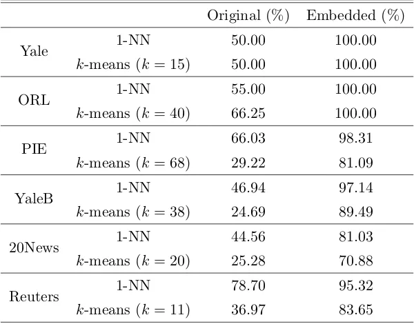
(interclass). The effectiveness of the proposed method is evaluated through comparison

with seven existing techniques for embedding learning, using four established databases

of faces, consisting of various poses, lighting conditions and facial expressions, as well as

two standard text datasets. The proposed method performs better than these existing

techniques, especially for cases with small sets of training data samples.

For fusion of low bit depth images, using low bit depth images instead of full images

offers a number of advantages for aerial imaging with UAVs, where there is a limited

transmission rate/bandwidth. For example, reducing the need for data transmission,

re-moving superfluous details, and reducing computational loading of on-board platforms

(especially for small or micro-scale UAVs). The main drawback of using low bit depth

imagery is discarding image details of the scene. Fortunately, this can be reconstructed

by fusing a sequence of related low bit depth images, which have been properly aligned.

To reduce computational complexity and obtain a less distorted result, a similarity

transformation is used to approximate the geometric alignment between two images of

the same scene. The transformation is estimated using a phase correlation technique.

It is shown that that the phase correlation method is capable of registering low bit

(3)

For 3D reconstruction from 2D images, a method is proposed to deal with the

dense reconstruction after a sparse reconstruction (i.e. a sparse 3D point cloud) has

been created employing the structure from motion technique. Instead of generating a

dense 3D point cloud, this proposed method forms a triangle by three points in the

sparse point cloud, and then maps the corresponding components in the 2D images back

to the point cloud. Compared to the existing methods that use a similar approach, this

method reduces the computational cost. Instated of utilising every triangle in the 3D

space to do the mapping from 2D to 3D, it uses a large triangle to replace a number

of small triangles for flat and almost flat areas. Compared to the reconstruction result

obtained by existing techniques that aim to generate a dense point cloud, the proposed

(4)

List of Figures

1.1 An example of embedding learning (taken from [13] but redrawn here):

representing a set of 3D data samples in a 2D feature space, while

pre-serving the local neighbour structure of each data sample in the original

3D feature space. . . 3

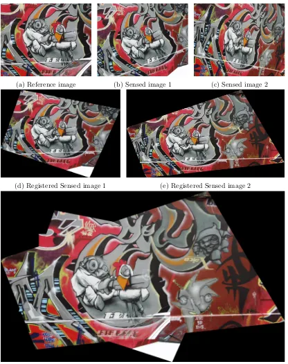
1.2 An example of image registration for the application area in image

mo-saicing . . . 5

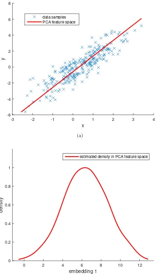
2.1 An example of embedding learning - PCA: (a) for a set of 2D data

sam-ples generated from a multivariate normal distribution, a PCA feature

space is calculated so that the corresponding variance is maximised. . . 19

2.2 An example of embedding learning - LPP versus PCA: (a) the projections

of the original 2D data in the LPP feature space have more discriminating

power, compared to those in the PCA feature space . . . 22

2.3 An example of embedding learning - LPP versus PCA (taken from [44]

but redrawn here): (a) compared to the feature space determined by

PCA, the feature space determined by LPP is less sensitive to the existing

outliers. . . 24

2.4 An example of embedding learning - FDA versus LPP versus PCA: (a)

the projections of the original 2D data in the FDA feature space possess

the most discriminant ability. . . 29

2.5 An example of embedding learning - LFDA versus FDA versus LPP: (a)

the projections of the original set in the LFDA feature space possess the

discriminant power, while preserving the local structures. . . 34

2.6 Comparison of the local structures in the original, LPP, FDA and LFDA

feature space: compared to the local structure in the original 2D feature

space, that in the resultant LFDA feature space has almost the same

structure, which demonstrates that LFDA is capable of preserving the

local structures. . . 35

2.7 An example of embedding learning - DNE versus LFDA versus FDA: (a)

the resultant feature space learned by DNE is almost the same as that

learned by LFDA (i.e. DNE is capable of discriminating data samples

(7)

2.8 An example of embedding learning - SELF versus LFDA versus PCA:

(a) the projections of the original 2D data in the SELF feature space

possess the most discriminant ability. . . 42

3.1 An example of an ideal pinhole camera. . . 50

3.2 An example of the same image under different distortions: translation,

Euclidean, similarity, affine, and projective. . . 55

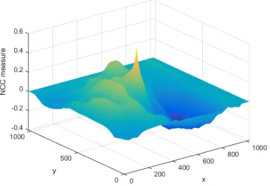
3.3 An example of registering a translation distorted image by NCC - the

reference and sensed images are shown in Figure 3.2a and 3.2b,

respec-tively: (c) the difference between the reference and registered images. . . 59

3.4 An example of registering a similarity distorted image by PC - the

refer-ence and sensed images are shown in Figure 3.2a and 3.2d, respectively:

(a) and (b) the spectrum magnitudes of the reference and sensed images

in the log-polar coordinates, respectively (f) the difference between the

reference and registered images. . . 63

3.5 An example of constructing DoG images (taken from [192] but redrawn

here): within each octave, Gaussian blurred images of the original

im-age are generated so that they are separated by a constant factork, as

shown on the left column. Then, the neighbouring blurred images are

subtracted to generate the DoG images, as shown on the right column.

After finishing the above process within an octave, the blurred image is

downsampling by a factor of 2, and then the process is repeated. . . 69

3.6 An example of scale-space images in an octave for the original image

shown in Figure 3.2a. . . 70

3.7 An example of DoG images, which corresponds to the scale-space images

shown in Figure 3.6: to make them move visible, all images are in the

jet colour map. . . 71

3.8 An example of detecting extremum in a DoG image (taken from [192] but

redrawn here): comparing the intensity value of a pixel location (marked

as X) to that of its 26 neighbours at the current and adjacent images

(marked as green circles). . . 72

3.9 An example of constructing a descriptor for a keypoint [192]: within

each 4×4 window, the gradient magnitudes and orientations of all pixel

locations are calculated to from an 8 bin histogram. . . 73

3.10 An example of constructing an 8 bin histogram [192]: a gradient

orienta-tion is added to the bin covering this orientaorienta-tion (i.e. each bin covers 45

degrees), and the amount added to the bin depends on the corresponding

gradient magnitude. . . 73

3.11 A RANSAC iteration example: estimating a model for a set of 2D data

(8)

3.12 Another RANSAC iteration example: estimating a model for a set of 2D

data samples, based on two randomly selected data samples. . . 79

3.13 An example of registering a projective distorted image by SIFT and

RANSAC - the reference and sensed images are shown in Figure 3.2a and

3.2f, respectively: (a) and (b) the SIFT features detected in the reference

and registered images (marked as cyan ×), respectively (c) and (d) the

feature correspondences detected before and after employing RANSAC,

respectively (f) the difference between the reference and registered images. 82

3.14 An example of interpolating intensity value by bilinear interpolation. . . 86

4.1 All the data samples in a single example class from each of the four face

databases: Yale, ORL, PIE, and YaleB. . . 105

4.2 Comparison of the class structures based on the proximity matrices

com-puted from the original data samples (the entire training sets were used). 109

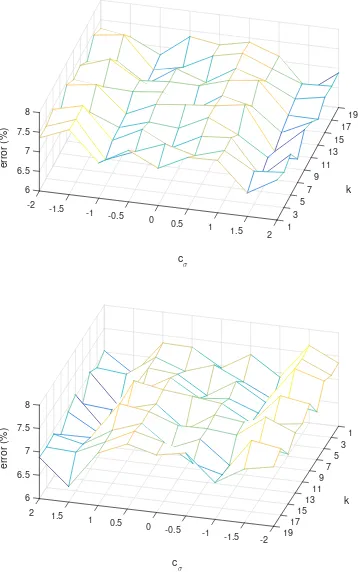
4.3 Sensitivity analysis of the performance of the proposed method to the

variations of the parameters kand σ (in terms of cσ), on YaleB. . . 111

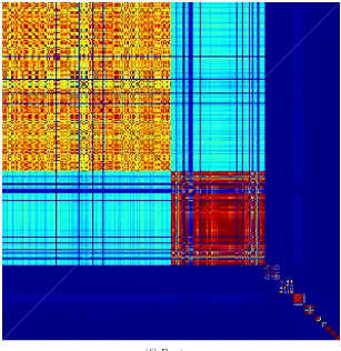
4.4 Comparison of the class structures based on the proximity matrices

computed from the embedded data samples generated by the proposed

method (the entire training sets were used). . . 114

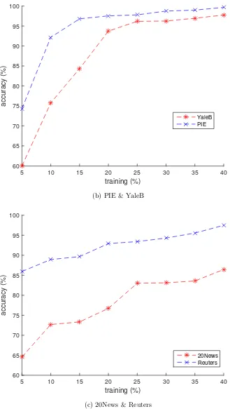
4.5 Performance of the proposed method, in terms of accuracy rate of

classi-fication and identiclassi-fication, on the six different datasets with varying the

number of data samples for training. . . 117

5.1 Examples of two 8-bit depth images and the corresponding 2-bit depth

images: Gaussian noise is present in the 8-bit depth images, and the

image structures are preserved in the 2-bit depth images. . . 122

5.2 A sequence of nine similarity distorted 2-bit depth images of the 8-bit

depth example image shown in Figure 5.1a (i.e. aerial image). . . 125

5.3 A sequence of nine similarity distorted 2-bit depth images of the 8-bit

depth example image shown in Figure 5.1c (i.e. Lena). . . 126

5.4 Registration results of the images shown in Figure 5.2. . . 127

5.5 Registration results of the images shown in Figure 5.3. . . 128

5.6 Original 8-bit depth images, and reconstructed results by fusing the

cor-responding aligned images shown in Figure 5.4 and 5.5. . . 129

5.7 The NCC and SSIM measures between the original and reconstructed

images: the reconstruction process was repeated 100 times, for different

bit depth images (i.e. from 1-bit to 7-bit). . . 130

5.8 Examples of an example under different levels of Gaussian noise and

without any blurring: the SD of Gaussian noise is varied from 8 to 64,

(9)

5.9 Examples of an example image under different levels of Gaussian noise

and a fixed Gaussian blur (i.e. the scaleσ = 1.6/√2): the SD of Gaussian

noise is varied from 8 to 64, with a constant step value of 8. . . 132

and a fixed Gaussian blur (i.e. the scale σ = 1.6): the SD of Gaussian

and a fixed Gaussian blur (i.e. the scale σ = 1.6×√2): the SD of

Gaussian noise is varied from 8 to 64, with a constant step value of 8. . 134

and a fixed Gaussian blur (i.e. the scaleσ = 1.6×2): the SD of Gaussian

1-bit depth images. . . 136

6.1 An example of forming triangles for a number of 3D points in a flat

region: (a) a number of 3D points in a flat region (i.e. they almost lie on

a common plane) (b) the projections of the 3D points in this common

plane (c) the triangles formed by employing the technique Delaunay

triangulation (d) the boundary points of this region (e) the triangles

(10)

6.2 An example of mapping a 2D image triangle to the corresponding

posi-tion in the plane determined by three 3D points. . . 150

6.3 The graf set of six 2D images of the same scene for generating a sparse

point cloud, by the SfM technique. . . 152

6.4 The bark set of six 2D images of the same scene for generating a sparse

6.5 The wall set of six 2D images of the same scene for generating a sparse

6.6 The vgm set of six 2D images of the same scene for generating a sparse

6.7 A sparse point cloud generated by employing the application VisualSFM

[300], based on the six 2D image shown in Figure 6.3. . . 156

6.11 A dense point cloud generated by employing the application CMVS [301],

based on the sparse point cloud shown in Figure 6.7. . . 160

6.15 The 3D reconstruction result by employing the proposed method, based

on the sparse point cloud shown in Figure 6.7. . . 164

(11)

Acknowledgement

First of all, I am extremely grateful to my primary supervisor, Prof. Jason Ralph, for his

support, advice and encouragement throughout the whole duration of my PhD study.

His deep insights helped me at various stages of my research, especially the useful

guidance during the difficult conceptual development stage. I also remain indebted

for his financial support. My sincere gratitude also goes to my co-supervisor, Dr.

Yannis Goulermas, for his invaluable insights and suggestions. I really appreciate his

willingness to meet me at short notice every time.

I wish to express my sincere appreciation to the other colleagues and friends who I

met during my time at the University of Liverpool, and those who have contributed to

this thesis and supported me in one way or the other. Special thanks here are due to our

postdoctoral researcher, Dr. Elias Griffith, whose help with MATLAB programming

was of utmost importance when I was in the early stages of my PhD study. I would also

like to take this opportunity to thank Dr. Tingting Mu and Prof. Stephen Marshall

-my viva examiners, for their very helpful comments and suggestions.

Last but not least, words cannot express the feelings that I have for my parents for

their constant unconditional support over the years - both emotionally and financially.

I would not be where I am today if it not for them, and for which I could never thank

(12)

Chapter 1

Introduction

1.1 Research Topics

There are three applications (i.e. embedding learning, image fusion, and 3D

recon-struction) considered in this thesis, but there are two main areas of work: embedding

learning and image registration. Embedding learning techniques aim to convert data

from a high dimensional representation to a lower one while preserving the intrinsic

geometry of the data, while image registration techniques aim to determine a

geomet-rical transformation that aligns two images of the same scene. Although they do not

seem directly related to each other at first, both of them are often included as

process-ing stages in applications of computer vision and other relevant areas of science and

engineering. More recently, embedding learning is used as a pre-processing stage to

enhance the performance of image registration, such as for medical imaging [1–3], and

in hyperspectral imaging [4, 5].

1.1.1 Embedding Learning for Classification

Handling measurements in a high dimensional mathematical space occurs frequently in

applications of machine learning, computer vision, data compression, and information

retrieval, as well as many other areas of science and engineering. The measurements are

often represented as feature vectors, and the vector space associated with these vectors

is called the feature space. For example, a statistical classification task commonly refers

to determining which of a set of categories (i.e. classes) one or more new measurements

(i.e. data samples) should belong to, on the basis of an existing set of measurements

whose corresponding category information (i.e. labels) is known. Many classical

clas-sification algorithms have been proposed, and they are widely employed, e.g. Neural

Networks (NNs) [6,7], Support Vector Machines (SVMs) [8,9] andk-Nearest Neighbour

(k-NN) classifiers [10, 11]. In real-world applications, data sets are usually represented

in high dimensional space. For example, a face image captured from a digital image or

a video frame often has many more degrees of freedom than that is required to define

(13)

or verification [12, 13]. Classifiers often suffer from some major problems as data

di-mension increases, such as increasing computational complexity, producing extremely

unreliable final results and so on [14, 15]. To overcome these problems, techniques that

aim to learn a compact representation of the original multivariate data sets are often

employed. These reduce dimensionality by eliminating irrelevant and/or redundant

information that is present in the original high dimensional data.

In general, embedding learning refers to the process of extracting a subset from a

set of data samples. For statistical classification, embedding learning can provide a

compact and meaningful representation for a set of data samples in a high dimensional

feature space by defining or determining a specific embedded subset of data samples

in a reasonably low dimensional feature space from the original (high dimensional)

set. The resulting embedded set should preserve some of the original properties and

characteristics of the data. An example of learning a specific set of 2D embeddings

from a set of 3D data samples is shown in Figure 1.1 [13], which was plotted by using

MATLAB 2014b. The manifold of the data set (i.e. the local neighbour structures)

that is present in the 3D space is unwrapped, as it is converted to a 2D space.

In the literature, a broad range of algorithms for embedding learning have been

proposed [15, 16]. Most algorithms differ from each other in the way that they preserve

important properties and characteristics that are present in the original set of data

samples during the learning process. The learning process refers to solving an

optimi-sation problem, which seeks to minimise or maximise an objective function, and whose

solution must satisfy a certain condition (i.e. a constraint). To achieve different

preser-vations of the important properties and characteristics, different objective functions

and the corresponding constraints are imposed according to the existing techniques.

Given a set of data samples that may have corresponding label information (i.e. which

class or classes each data sample belongs to), existing methods can be divided into the

following three categories, based on whether to utilise the label information and what

type of the label information is available. The first category is unsupervised learning,

where the techniques compute embeddings based only on certain feature properties and

characteristics that exist in the original data set, regardless of whether the

correspond-ing label information exists. The embedded set learned by unsupervised techniques is

a compact and informative representation of the original set which is based only on

features. The second category is supervised learning techniques, where the techniques

utilise the feature data and the corresponding label information when embeddings are

being constructed. The resultant supervised embeddings outperform unsupervised ones

in two ways: one is the grouping ability of the ones in the same class (i.e. keeping

in-terclass ones close together), and the other is the separation ability of the ones from

different classes (i.e. forcing interclass ones to move far apart). The last category is

(14)

15 10 5

x

0 -5 -10 -20 -10

y

0 0

5 15 20

10 25 30

10

z

(a) A set of 3D data samples

embedding 1

-0.04 -0.03 -0.02 -0.01 0 0.01 0.02 0.03

embedding 2

-0.04 -0.03 -0.02 -0.01 0 0.01 0.02 0.03 0.04

[image:14.612.145.489.91.654.2]

(b) An embedded set of 2D data samples

(15)

the label information is not complete (i.e. only part of the data set is labelled). Most

of these algorithms are some kind of combination of an unsupervised learning method

and a supervised one, i.e. employing an unsupervised learning method to consider all

the data samples and a supervised one to deal with only the labelled data samples.

The final performance of semi-supervised embedding learning methods are enhanced

compared to unsupervised learning, due to the employment of the supervised learning

techniques and the use of additional information (labels).

1.1.2 Image Registration & Its Application in 3D Reconstruction

Image registration is a fundamental problem in applications of image analysis related

areas. It aims to find one or more spatial transformations, so that two or more images

(commonly one reference image with one or more sensed images) of the same scene can

be geometrically aligned. Although the images are of the same scene, they differ from

each other because they may be taken at different times, from different viewpoints,

and/or by different sensors [17, 18]. For instance, in medicine, images taken from

dif-ferent modalities (i.e. using difdif-ferent wave bands, such as X-ray radiography, Magnetic

Resonance Imaging (MRI), medical ultrasonography and so on) are aligned to assist

di-agnosis. Image registration has become a crucial stage in tasks such as remote sensing,

medical imaging and computer vision, where final information is based on combining a

number of images. An example of image registration for image mosaicing [19] is shown

in Figure 1.2.

Generally, in 2D images, there are three major types of variations in images that

make them look distinct [17]. The first type of variation is caused by the process

of image acquisition, which leads to image misalignment. The second variations are

changes in the intensity values, due to changes in lighting conditions or relative contrast

in different modalities. The last type of variation is caused by changes in the scene,

such as moving objects. A spatial transformation between two images is sufficient

to remove the first type of variation, but not the other two types of variation. They

generate a more difficult problem in image registration, since an exact match is difficult

to achieve [17]. The problem would not be critical, as long as the changes in intensity

values are relatively small compared to the original intensity values, and the moving

object is not the object of interest in the taken images. As shown in Figure 1.2d, the

part of a car in the bottom right of the image (white area) is not removed after applying

image registration. Also as shown in Figure 1.2f, the final result of image mosaicing is

reasonable, because the part of the car is not the main object of interest in the three

images.

Over the years, a broad range of techniques for image registration have been

pro-posed for a wide variety of areas [17, 18, 20, 21]. Unfortunately, because images to be

(16)

(a) Reference image (b) Sensed image 1 (c) Sensed image 2

(d) Registered Sensed image 1 (e) Registered Sensed image 2

[image:16.612.114.530.67.592.2]

(f) Final result of image mosaicing

Figure 1.2: An example of image registration for the application area in image mosaicing

no one existing method that can achieve an optimal performance when the alignment is

across different types of sensor, platform and/or problem [18, 22]. Existing techniques

for image registration can be classified into two major categories: area based methods

and feature based ones. The area based methods process images without detecting any

(17)

the image) of predefined size are used for the estimation of corresponding

transforma-tion models, which describes mathematical relatransforma-tionships between images for alignment.

However, because they only make direct use of matching image intensity values, with

no analysis of image structures, they are sensitive to the changes in intensity value.

Compared to area based methods, feature based ones work by detecting more robust

features: usually sets of points or small blocks detected in the reference and sensed

images. The aim of these methods is to find the pairwise correspondence between the

detected features in the different images, using either the spatial relations or various

feature descriptors.

In general, the process of image registration can be divided into the following four

stages: detecting features, where the information in the images is useful for matching

is extracted; matching features, where the correspondences are established between the

features detected in the reference and sensed images; estimating the transformation

model, where the type and the parameters in the spatial transformation are estimated,

on the basis of the established correspondences of the detected features; and

trans-forming & resampling images, where the sensed images are transformed and resampled

according to the estimates of the spatial transformation [18].

Detecting Features Features commonly refer to significant areas in images, i.e. salient regions, lines or even points, which are manually selected or, preferably,

auto-matically detected [17,18]. Nevertheless, the features should be distinctive, expected to

be easily detectable and somehow stable, i.e. the same features detected from different

images should share sufficient common elements, even in situations where images do

not cover the exactly the same scene and/or the objects present in images are occluded.

Ideally, any applicable method should be able to detect the same features in all of the

possible images of the same scene, and be insensitive to any assumed type of geometric

deformation and/or additive noise.

Matching Features In this stage, the features detected in different images are matched to each other. The matching process is based on either various measures

of image intensity values between the detected features and the several nearest

neigh-bours, or a similarity measure of the descriptors constructed according to the detected

features. Since any incorrectly matched pairs of features will cause the performance to

suffer in the following stages, the algorithms proposed for matching features should be

robust. Some existing techniques (i.e. area based methods) merge the current stage

with the next one, because once the pairs of feature correspondences have been

de-termined, they can directly estimate the parameters required by the transformation

(18)

Estimating Transformation Models The spatial transformation that can geomet-rically align two images is estimated in this stage. Based on the prior information about

the assumed transformation model, the parameters required by the spatial

transforma-tion are computed using the established matched pairs of feature correspondences. The

estimated model of the spatial transformation should result in a reasonable

transforma-tion, where the corresponding matched pairs are located as close as possible. If there is

no prior information available, the estimated model should be both flexible and general

enough to handle all possible spatial transformations for geometrical alignment.

Transforming & Resampling Images After the model of a spatial transformation has been estimated, the images can be geometrically aligned by mapping the sensed

image(s) into the spatial coordinate of the reference image. Since the new pixel

coordi-nate of the registered image is determined according to that of the reference image, a

non-integer pixel location is often generated, where no appropriate intensity value can

be assigned directly. To address this problem, the sensed images are often resampled

employing an appropriate intensity interpolation technique. The choice of the intensity

interpolation technique depends on the trade-off between the registration accuracy and

the computational complexity. In general, the technique of bilinear interpolation is

sufficient enough for practical applications [18].

3D Reconstruction from 2D Images

3D reconstruction from 2D images is a challenging task in computer vision and

com-puter graphics. It represents a process of obtaining 3D information about the geometry

of a scene from 2D images of this scene. Depth data is the 3D component missing from

given 2D images. To recover depth data, image registration serves as the key part. This

is because a 3D point can be reconstructed by triangulation [23], with the use of its

cor-responding pixel locations in the 2D images that have already been matched through

image registration. To apply triangulation methods, it is an important prerequisite

that the pose and calibration of each camera used should be determined. Traditional

methods require a priori information about 3D positions, such as the 3D location and

pose of camera, or the 3D location of ground control points [23]. However, there is

a method called Structure from Motion (SfM) [23, 24], which can simultaneously and

automatically get the camera pose and scene geometry. It is achieved by employing a

method called bundle adjustment [25, 26], which is based on matched pixel locations

extracted from multiple 2D images that are overlapping and offset.

1.2 Novel Contributions

For embedding learning, a new approach has been proposed to try to overcome the

(19)

underlying structure of a given dataset. It attempts to generate a feature space formed

by distinct feature(s) of each class, which could potentially enhance the grouping of the

data samples in this class while separating them from those in the remaining classes.

Compared to the existing techniques that try to find distinguishing features, each of

which attempts to separate all classes, this approach focuses on finding the distinct

characteristics of one class at a time. It results in the following two contributions:

Firstly, the idea of One-Vs-All (OVA) [27, 28] which decomposes a multiclass

classi-fication problem into several binary ones is applied to embedding learning. It finds

distinct feature(s) for each class individually, so that the data samples in this class can

be uniquely defined, and then separated from those in the remaining ones. Secondly,

to overcome the problem of the imbalanced number of data samples when addressing

final optimisation, a weighted pairwise constraint indicator is proposed to balance the

contributions of the data samples from a target class and those from the remaining

classes.

For image registration, to reduce the usage of on-board computational resources

in small Unmanned Aircraft System (UAS) platforms, an approach can be employed

using low bit depth images instead of full bit depth ones. It only transmits the first

few Most Significant Bits (MSBs) of image data, and it is based on the assumption

that the most important information of each image (e.g. the main structure of the

scene) is contained in the MSBs. To address the problem that low bit depth imagery

can discard image details within the Least Significant Bits (LSBs), it has been found

that the discarded details may be reconstructed by fusing a sequence of related low

bit depth images if there is sufficient noise in the images, when the temporal sequence

has been aligned by image registration [29]. Additionally, the area based registration

method Phase (Fourier) Correlation is employed here, to achieve a low computational

complexity. It results of the following two contributions: Firstly, the phase correlation

method is demonstrated to be capable of registering low bit depth images (up to a

distortion caused by a similarity transformation), without any modification, or any pre

and/or post-processing. Secondly, the image details discarded due to quantisation of

low bit depth imagery can be reconstructed with high fidelity by fusing a number of

related low bit depth images with noise.

For 3D reconstruction from 2D images, a new approach has been proposed to achieve

a good trade-off between the reconstruction details and the computational load. Unlike

the common approach that maps 2D image triangles one by one to the 3D scene, it forms

several large triangles to describe a flat or almost flat region. Each of the large triangles

actually covers a number of small triangles, and they are formed based on the boundary

points of the region. It results in two contributions. Firstly, to describe a region with a

number of triangles, the triangles formed based on boundary points of this region can

(20)

triangles can achieve almost same performances when describing this region, compared

one that based on all small triangles at considerably lower computational cost.

1.2.1 Publications

Parts of the above novel contributions have been presented at conferences and published

in a journal paper:

1. Y. Chi, E.J. Griffith, and J.F. Ralph. Low bit depth images for small,

micro-scale UAVs. In 6th International Conference on Imaging for Crime Detection

and Prevention (ICDP 2015), London, UK, 15-17 Jul. 2015, pages 21–26. IET,

2015

2. Y. Chi, E.J. Griffith, J.Y. Goulermas, and J.F. Ralph. Binary data

embed-ding framework for multiclass classification. IEEE Trans. Human-Mach. Syst.,

45(4):453–464, 2015

3. Y. Chi, E.J. Griffith, J.Y. Goulermas, and J.F. Ralph. Binary data embedding

framework for face recognition. In 5th International Conference on Imaging for

Crime Detection and Prevention (ICDP 2013), London, UK, 16-17 Dec. 2013,

pages 102–107. IET, 2013

4. E.J. Griffith, Y. Chi, M. Jump, and J.F. Ralph. Equivalence of BRISK descriptors

for the registration of variable bit-depth aerial imagery. In 2013 IEEE

Interna-tional Conference on Systems, Man, and Cybernetics (SMC), Manchester, UK,

13-16 Oct. 2013, pages 2587–2592. IEEE, 2013

1.3 Structure of Thesis

This thesis is further divided into six chapters:

• Chapter 2,Embedding Learning for Classification, describes the main con-cepts of embedding learning for classification, and examines the commonly used

techniques in unsupervised, supervised and semi-supervised embedding learning,

as well as the embedding learning techniques for multi-label classification.

• Chapter 3,Image Registration & Its Application in 3D Reconstruction, shows how a pinhole camera model leads two 2D images of the same scene to be

related by a transformation model, and examines the commonly used techniques

for registering 2D images - both area based and feature based. Additionally, the

structure from motion technique is examined here, it reconstructs a 3D scene

(21)

• Chapter 4, Binary Data Embedding Framework, describes the motivation and technical details of the work that has been done for embedding learning,

and additionally an experimental evaluation is conducted to demonstrate the

performance of the proposed method.

• Chapter 5,Image Reconstruction by Fusing Low Bit Depth Image, pro-vides the motivation and whole process of the work that has been done for image

reconstruction, as well as an evaluation of the reconstruction process to show the

reconstruction quality.

• Chapter 6,3D Scene Reconstruction from 2D images, presents the motiva-tion and whole process of the work done that has been done for 3D reconstrucmotiva-tion,

and additionally an experimental evaluation is conducted to demonstrate the

per-formance of the proposed method.

(22)

Chapter 2

Embedding Learning for

Classification

This chapter, describes the background of embedding learning and introduces the

stan-dard mathematical notation that will be used in later chapters. Subsequently, a broad

review of the well known techniques for embedding learning is presented.

2.1 Background

Embedding learning aims to embed a set of data samples into a lower dimensional

fea-ture space that can capfea-ture the meaningful degrees of freedom present in the data. It

has become an essential processing stage in many applications in science and

engineer-ing [14]. In recent years, a wide range of algorithms for embeddengineer-ing learnengineer-ing have been

proposed [15, 16]. The existing algorithms can be split into two different categories,

based on whether there is an explicit relation between a set of data samples and its

corresponding set of embeddings. One is nonlinear learning, where the techniques, such

as Locally Linear Embedding (LLE) [13], Laplacian Eigenmaps (LE) [34], and other

algorithms proposed in [12, 35–40], generate resultant embeddings that have no explicit

relation to the original set. In other words, there is no linear relationship between

the original set and the corresponding embedding results. The other category is linear

learning, where there exists an explicit relation, and it is captured by a linear

map-ping/projection function. Here, the focus will be on the methods in the later category,

since they are usually insensitive to the parameters [41], have lower computational

complexity [41], and are simpler and straightforward for real-time applications. For

instance, for the purpose of classification, once a linear mapping/projection function

has been determined from a training set (i.e. a set of data used for learning), it can be

used for mapping/projecting any data sample in the corresponding test set (i.e. a set

of data used solely for testing generalisation performance) to the same feature space,

for further identification or verification.

(23)

generate embeddings only based on specific feature properties and characteristics of

a set of data samples, without explicit knowledge of the identifies or classes of the

data. For example, Principal Component Analysis (PCA) [42] aims to yield an

orthog-onal projection function, so that the corresponding embedding results are uncorrelated

to each other, and the corresponding total variance is maximised. Latent Semantic

Indexing (LSI) [43] attempts to obtain a lower rank approximation to represent the

original set. Both methods take into account the global structure of the original set

when determining the mapping functions, but not the local structure. As a result, it

is likely that the local structures of the resultant embeddings become distorted. To

overcome this problem, various methods using manifold learning and spectral analysis

have been developed to take into account the local structure information when

generat-ing embeddgenerat-ings [12, 13, 34–38, 40, 44–49]. For example, Locality Preservgenerat-ing Projections

(LPP) [44], Orthogonal Locality Preserving Projections (OLPP) [45] and Orthogonal

Neighbourhood Preserving Projections (ONPP) [45] focus more on the local structures

of the original set to preserve the essential geometry. This can be captured by pairwise

proximity information based on constructed graphs for the local neighbours of each

data sample [14]. These techniques differ from each other through different

assump-tions on how to construct graphs of local neighbours and enforce constraints: ONPP

assumes that each data sample can be represented by a linear combination of its local

neighbours, while LPP and OLPP employ similarity measures to capture graphs of

lo-cal neighbours. Additionally, both OLPP and ONPP indicate that each dimensionality

of the resultant linear mapping/projection function should be orthonormal.

When a set of data samples possesses a good arrangement between the features and

the corresponding classes (i.e. the data samples in the same class are located nearby,

while those from different classes are located far away), the above unsupervised methods

can obtain a good and informative representation of the original set, based only on

certain feature properties and characteristics, and no local information. However, for

a real world dataset, a good arrangement may not always hold. Therefore, there may

exist confusing data samples in the original set (i.e. data samples from different classes

are located nearby, and/or those in the same class are located far away), and then both

global and local structures of the original set become unreliable due to the existence of

the confusing data samples. The resultant embeddings, which are only learned on the

basis of feature properties and the characteristics of the original set, may degrade the

final performance. Additionally, the local neighbour information, which is utilised by

some unsupervised methods, is based on one type of distance measure (metric) between

each data sample and its neighbours in the original feature space. It may be influenced

when there exists a bad arrangement between the features and the labels. As a result,

these methods may fail to overcome the problem, and can increase the misclassification

(24)

space may get projected into a wrong class in the embedded feature space.

To avoid such problems, techniques that use the set of data samples and the

cor-responding label information have been proposed. These techniques are supervised

learning methods. They improve the grouping ability of the data samples in the same

class (i.e. intraclass), whilst increasing the separation ability of those from different

classes (i.e. interclass). Most of the supervised methods attempt to embed a set of

data samples, so that the data samples of intraclass are made to be close together and

the interclass data samples are as far apart as possible. For example, both Fisher

Dis-criminant Analysis (FDA) [50] and Maximum Margin Criterion (MMC) [51] achieve

this based on the additional use of the label information to capture the within-class

and between-class scatters (i.e. the estimates of the corresponding covariance matrices)

for respective intraclass and interclass information of the original set. Both methods

encourage all of the data samples of the same class to stay close together and those of

different classes to move apart, with a slight difference in the way of formulating each

objective function - FDA utilises the ratio of the two scatters, while MMC [51] utilises

the difference between the two scatters (intra- / interclass). Various other methods

have been proposed [52–66], and the majority of these are based on using rules similar

to that of FDA and MMC with slight variations or incorporating the label

informa-tion into the pairwise proximity informainforma-tion modified by the unsupervised methods.

For example, Marginal Fisher Analysis (MFA) [52], Discriminative Locality Alignment

(DLA) [53], and Discriminant Neighbourhood Embedding (DNE) [54] encourage only

the neighbouring data samples of intraclass and interclass to be nearby and far away,

respectively. They share the same idea, but differ from each other in the way that they

impose each objective function and constraints. MFA [52] is a variant of FDA, where it

considers local neighbour information by redefining the between-class and within-class

scatters, on the basis of k-NN information. DLA [53] works similar to MFA, but it

employs a criterion whose form is similarly to that of MMC (a difference rather than

a ratio). DNE [54] incorporates the label information into the graphs of local

neigh-bourhoods constructed by OLPP. Local FDA (LFDA) [57] is another variant of FDA,

where it keeps the neighbouring data samples of intraclass close, while for the data

samples of interclass, it works more strictly - it makes all of them move apart.

Repul-sion OLPP (OLPP-R) [60] uses the neighbourhoods differently compared to LFDA: it

keeps all of the data samples of intraclass close, while the neighbouring data samples

of interclass move apart. Repulsion ONPP (ONPP-R) [60] and Discriminative ONPP

(DONPP) [63] are more complex, both of them preserve the local data structure within

each class separately, while encouraging the neighbouring data samples of interclass to

move apart. They differ from each other through the use of different reconstruction

weights. ONPP-R [60] uses reconstruction weights that are calculated for all data

(25)

data samples that are close by in the original feature space. DONPP [63] uses

recon-struction weights which are calculated based on the assumption that each data sample

can be reconstructed from the remaining ones in its class.

The fully supervised learning techniques make the use of labelled data samples

when determining optimal projection functions. But in some situations, labelling data

samples is difficult, expensive or time consuming, so only a small number of them are

actually labelled. Employing unsupervised learning techniques in such cases may

gen-erate unreliable results, while employing supervised learning techniques with only the

labelled data samples may fail to discover the actually meaningful structures, due to

the small sample size. To address this problem, a group of techniques, called

semi-supervised learning have been developed to use both unlabelled and labelled data

sam-ples to build a better mapping function [63, 67–73]. The simsam-plest way to approach

semi-supervised learning is to combine an unsupervised technique and a supervised

one, i.e. using the unsupervised technique to deal with all data samples (both

un-labelled and un-labelled), while the supervised technique deals with the un-labelled data

samples. For example, Semi-supervised DONPP (SDONPP) [63] combines ONPP with

DONPP, SEmi-supervised LFDA (SELF) [69] combines PCA and LFDA, while

Semi-Supervised FDA (SSFDA) [68] and Semi-Semi-Supervised MMC (SSMMC) [68] combine

OLPP with FDA and MMC, respectively. There are other different ways to achieve

semi-supervised learning, for example methods described in [71] and [72] attempt to

learn predicted labels. A broader review on semi-supervised learning techniques can be

found in [73–75].

The algorithms for supervised and semi-supervised learning typically only aim for

single label classification, where each data sample is assigned exactly one label. For

more complex classification problems, data samples are extended from single label to

multi-label, i.e. a data sample simultaneously belongs to two or more classes. In such

cases, the above algorithms are no longer applicable. To address this problem, a variety

of algorithms for multi-label classification have been proposed [76–87]. A direct way to

achieve embedding learning for multi-label classification is to find a optimal approach

to balance some kind of statistical measure (e.g. covariance or correlation coefficient)

of the embedding results and the corresponding multi-label information. For

exam-ple, Partial Least Squares (PLS) [76, 77] attempts to maximise the covariance between

the resultant embeddings and the corresponding multi-label information. Canonical

Correlation Analysis (CCA) [79, 80] works similarly to PLS. Instead of employing

co-variance, it aims to maximise the correlation coefficient. A recent review of the existing

(26)

2.1.1 Definitions

The input to a method on linear embedding learning is a training set ofndata samples

of dimensiond, where it is denoted by an n×dmatrix X, as:

X= [x1,x2, . . . ,xn]T (2.1)

whereT denotes the transpose operator, andxi= [xi1, xi2, . . . , xid]T corresponds to the ith data samples in the training set. The ntraining data samples belong to cdifferent

classes, and this class information is modelled as ann×cbinary matrix Y as:

Y= [y1,y2, . . . ,yn]T (2.2)

whereyi = [yi1, yi2, . . . , yic]T indicates which of the c different classes (C1, C2, . . . , Cc)

that theith training data sample belongs to, and theijth element yij is defined as:

yij =

1 ifxi ∈Cj (i.e. xi belongs to Cj)

0 otherwise (2.3)

The number of the training data samples from the ith class Ci is denoted by ni (i =

1, . . . , c). The corresponding test set consists of mdata samples of dimension d, and it

is denoted by am×dmatrixXe, as:

e

X= [x_e1,ex2, . . . ,exm]

T _(2.4)

wherex_ei = [xei1,exi2, . . . ,exid]

T _{corresponds to the}_i_{th test data sample.}

The objective of the techniques for linear embedding learning is to construct a

linear mapping/projection functionψ:Rd→Rkfrom either only the training setXor both the training setX and the corresponding label informationY. The functionψis denoted by ad×kmatrixV. It generates a training set of nembeddings of dimension

k(k < d), denoted by a n×k matrixZ, as:

Z=XV = [z1,z2, . . . ,zn]T (2.5)

where zi = VTxi = [zi1, zi2, . . . , zik]T corresponds to the ith data sample in the

em-bedded training set. In the emem-bedded feature space, the dimensionality of the training

set is reduced, and additionally the manifolds in the low dimensional space that the

training data samples lie on should be recovered, as well as the discrimination between

the data samples from different classes must be enhanced [14]. Then, through the same

determined mapping/projection functionV, the corresponding test setXe are projected

to the same embedded feature space, denoted by am×k matrixZe, as:

e

Z=XVe = [_ez₁,_ez₂, . . . ,_ez_m]T (2.6)

wherez_ei=VTxei = [zei1,ezi2, . . . ,ezik]

T _{corresponds to the}_i_{th embedded test data}

sam-ple. The dimensionality of the data samples in the test set is reduced and the

(27)

discriminability of the embedded test data samples is a way to measure the final

per-formance of the determined mapping/projection function.

To give a better review of the existing embedding learning techniques, the well

known techniques on unsupervised, supervised and semi-supervised learning are each

examined in detail. Although the concept of multi-label learning is beyond the scope of

this thesis, some commonly used techniques for multi-label classification are listed for

completeness. Sometimes, since the meaningful structure of a data set lies on a

nonlin-ear space, the linnonlin-ear embedding lnonlin-earning techniques will fail to discover the nonlinnonlin-ear

structure. To overcome this problem, some techniques are developed to increase the

power of the proposed algorithms for embedding learning by extending them to

non-linear space. Some commonly used techniques for nonnon-linear extension are also listed.

2.2 Unsupervised Learning Techniques

The unsupervised learning techniques determine mapping/projection functions on the

basis of using some feature properties and characteristics of a set of data samples.

Through the mapping/projection functions that are determined, the algorithms aim to

provide a good and informative representation of the original set.

Principal Component Analysis

Principal Component Analysis (PCA) [42], also known as the Karhunen-Loeve

Trans-form (KLT) [88], is one of the most widely used methods for linear embedding learning.

PCA constructs a d×k orthogonal projection matrix V, to maximise the variance of all the embedded data samples [42]. It has a number of advantages [89]: reducing

the number of dimensions without much loss of the original information, removal of

redundancy, and reduction of noise. For the training set X, the maximisation of the variance of all the embeddings can be formulated as:

arg max

zi∈Rk 1

n−1

n X i=1

zi−

1 n n X j=1 zj 2 2 (2.7)

wherek · k₂ donates the 2-norm or Euclidean norm, and the objective function can be

reformulated as [55]:

n X i=1

zi−

1 n n X j=1 zj 2 2 = n X i=1 

zi−

1 n n X j=1 zj   T 

zi−

1 n n X j=1 zj   = tr    n X i=1 

z_i−

1 n n X j=1 zj   

z_i−

(28)

Then, the maximisation problem in (eq. (2.7)) is equivalent to the following:

arg max

V∈Rd×k_,_VT_V₌_I k×k

tr    n X i=1 

VTxi−

1

n n

X

j=1

VTxj



 

VTxi−

1

n n

X

j=1

VTxj





T



 (2.9)

where tr[·] is the trace operator, and the optimisation problem above can be

reformu-lated as:

arg max

trVTStV

(2.10)

whereStis defined as:

St= n

X

i=1



xi−

1 n n X j=1 xj   

xi−

1 n n X j=1 xj   T (2.11)

Stis called the total scatter matrix of the training setX[55]. Stabove can be expressed

more succinctly, as:

St=XT

In×n− 1 n1n×n

T

In×n− 1 n1n×n

X

=XT

In×n−

1

n1n×n

X (2.12)

whereIn×n−_n11n×nis the n×ncentring matrix.

The optimal projection matrixV∗= [v1,v2, . . . ,vk] can be obtained by employing

Lagrangian multipliersλi (i= 1, . . . , k) [55]:

L(vi, λi) =vTi Stvi−λi(viTvi−1) (2.13)

Next the derivative with respect tovi is taken:

∂L(vi, λi) ∂vi

=Stvi+STtvi−2λivi (2.14)

using the fact that St is a symmetric matrix, and the derivative result is set to zero,

thus the following is obtained:

Stvi=λivi (2.15)

Clearly, the equation above is a standard eigenvalue problem. The optimal projection

matrix V∗ is obtained by Singular Value Decomposition (SVD) [90], whose columns [v1,v2, . . . ,vk] are the k standard eigenvectors of St, corresponding to the k largest

standard eigenvalues [λ1, λ2, . . . , λk].

An example of PCA embedding learning for a set of data samples in 2D is shown

in Figure 2.1. The data samples are generated from a multivariate normal distribution

with a mean of (0.392,0.207) and a covariance of [1,1.5; 1.5,3], and then the PCA

(29)

data samples are projected from the original 2D feature space into this new 1D feature

space, the corresponding variance is maximised.

To visually analyse the projected data samples in the determined 1D feature space,

the corresponding density can be estimated as follows: First, let mline represent the

slope or gradient of the determined line, then the projected coordinate of an arbitrary

data pointxi can be calculated as:

yi= [cos(arctan(mline)),sin(arctan(mline))]×[xi1, xi2]T (2.16)

Since a linear shift in the projected coordinate set Y will not have any effect on the final result of density estimation, Y can be shifted linearly so that it starts from the value of 0. This can be simply achieved by:

Y=Y−min(Y) (2.17)

where min(·) returns the minimum value. Next, a histogram, with the number of bins

being 20, is contracted based on the shifted coordinate setY. Finally, a density function is estimated by fitting it to the contracted histogram, based on the assumption that

the data samples are in a nonparametric kernel-smoothing distribution.

Latent Semantic Indexing Latent Semantic Indexing (LSI) [43] is a method that works very similarly to PCA. It operates like PCA, but without the process of centring

the data samples eq. (2.12). A document-term matrix, which identifies the occurrences

of a number of unique terms within a dataset generated by a collection of

document-like data (e.g. 1 indicates a term occurs, while 0 otherwise), is usually a sparse matrix.

Thus, the centring process (i.e. subtracting off the mean) will result in losing the

original sparseness present in the document-term matrix, and then increasing the cost

of processing and/or storing it. LSI was developed for text processing, however due

to its similarity to PCA, it has been applied to a variety of application areas, such

as information retrieval. Based on (2.10) and (2.12), LSI gets its optimal projection

function by solving the following optimisation problem:

arg max

trVTXTXV (2.18)

Locality Preserving Projection

Both PCA and LSI construct the optimal mapping functions based on preserving the

global structure of the original set, because of this it is likely that the corresponding

local structures are distorted. Locality Preserving Projection (LPP) [44] is a method

that was proposed to focus more on the local structures of the original set, when

con-structing the optimal mapping function. It is developed through the pairwise proximity

(30)

x

-3 -2 -1 0 1 2 3 4

y

-6 -4 -2 0 2 4 6 8

data samples PCA feature space

(a)

embedding 1

0 2 4 6 8 10 12

density

0 0.2 0.4 0.6 0.8 1

estimated density in PCA feature space

[image:30.612.157.474.86.646.2]

(b) the estimated density of the projected data samples in the PCA feature space

(31)

represent the local structures. As a result, it is likely that a search of nearest

neigh-bours in the resultant embedding feature space will yield a similar result, compared to

that in the original high dimensional feature space. This makes LPP particularly

use-ful in applications such as information retrieval, where a search of a nearest neighbour

is ultimately needed [44]. LPP has been demonstrated to have more discriminating

power than PCA and be insensitive to the presence of outliers [44]. The advantages are

both shown as an example of embedding learning between PCA and LPP in Figure 2.2

and 2.3. In Figure 2.2a, the data samples of two different classes are generated from

two different multivariate normal distributions, with different means (0.366,0.620) and

(7.366,6.620) while a common covariance [1,1.5; 1.5,3]. Comparing Figure 2.2b and

2.2c, it can be seen that the two estimated densities shown in Figure 2.2c have less

overlap region. It means that in the LPP feature space, the projected data samples

have better separation performance. Because a suitable distance is maintained between

the data samples of the two classes, a simple classifier based on nearest neighbour search

(e.g. 1-NN, which simply assigns a test data sample to the class of its nearest

neigh-bour) is powerful enough to achieve class discrimination. PCA feature space, although

it maximises the variance, it distorts the good arrangement between nearest neighbour

and class label (i.e. a data sample and its nearest neighbour are from the same class).

This makes the 1-NN classifier fail to achieve a good performance. The LPP feature

space preserves the local structures, which results in more discriminating power. In

Figure 2.3a, the data samples are generated from a multivariate normal distribution

with a mean of (0.879,0.548) and a covariance of [1,1.5; 1.5,3], while several outliers

are added to the Gaussians. For the same reason, the resultant LPP feature space

is less sensitive to outliers, compared to the PCA one. However, LPP may lead to

unsatisfying effectiveness due to the constructed graph of local neighbours [41]. This is

because the local neighbourhood graph is generated based on adopting the Euclidean

distance as the similarity measure between data samples, while the Euclidean distance

cannot adequately describe the intrinsic geometry of the manifold structure in the real

word [41].

LPP is a linear approximation of Laplacian Eigenmaps (LE) [34], where a linear

constraint is imposed between the original set and the determined mapping/projection

function. It attempts to minimise the pairwise distance errors between all the data

sam-ples in the embedded feature space, and then for the training setX, the corresponding minimisation problem is defined as:

arg min

zi∈Rk

n

X

i,j=1

wijkzi−zjk2₂ (2.19)

where the imposed linear constraint is zi =VTxi, and wij is the ijth element of the n×n weight matrix W. wij is defined based on a similarity or closeness measure

(32)

used similarity or closeness measures for weight matrix W are listed in appendix A.

wij is only nonzero when theith and jth data samples are connected. Commonly, two

different ways are used to define whether a connection exists. One is when theith data

x

-4 -2 0 2 4 6 8 10 12

y

-4 -2 0 2 4 6 8 10 12

data samples of class 1 data samples of class 2 PCA feature space LPP feature space

(a)

embedding 1

0 2 4 6 8 10 12 14 16 18

density

0 0.2 0.4 0.6 0.8 1

in PCA Feature Space

estimated density of class 1 estimated density of class 2

(33)

embedding 2

0 2 4 6 8 10 12

density 0 0.2 0.4 0.6 0.8 1

in LPP Feature Space

(c) the estimated densities of the projected data samples in the LPP feature space

Figure 2.2: An example of embedding learning - LPP versus PCA: (a) the projections of the original 2D data in the LPP feature space have more discriminating power, compared to those in the PCA feature space

sample is the mutual or undirected k-NN of the jth one, and vice versa; the other is

when a specific measure of the distance between theith andjth data samples is below

a pre-defined threshold. Based on the work in [44], the objective function above can

be reduced to:

1 2

n

X

i,j=1

wijkzi−zjk2₂ =

1 2   n X i,j=1

wijzTi zi+ n

X

i,j=1

wijzTjzj− n

X

i,j=1

wijzTi zj− n

X

i,j=1

wijzTjzi

  = n X i,j=1

wijzTizi− n

X

i,j=1

wijzTi zj

=

n

X

i=1

zT_i

  n X j=1 wij 

z_i−

n

X

i,j=1

zT_i wijzj

= tr   n X i=1 zi   n X j=1 wij 

zT_i −

n

X

i,j=1

ziwijzTj





= tr

ZTDZ−ZTWZ

(34)

whereD is ann×ndiagonal matrix, with its ith diagonal element diibeing:

dii= n

X

j=1

wij (2.21)

x

-3 -2 -1 0 1 2 3 4

y

-10 0 10 20 30 40 50 60 70 80

data samples of class 1 data samples of class 2 PCA feature space LPP feature space

(a)

embedding 1

0 10 20 30 40 50 60 70 80

density

0 0.2 0.4 0.6 0.8 1

in PCA Feature Space

(35)

embedding 2

0 1 2 3 4 5 6 7

density

0 0.2 0.4 0.6 0.8 1

in LPP Feature Space

(c) the estimated densities of the projected data samples in the LPP feature space

Figure 2.3: An example of embedding learning - LPP versus PCA (taken from [44] but redrawn here): (a) compared to the feature space determined by PCA, the feature space determined by LPP is less sensitive to the existing outliers.

and it can be formed from [15]:

D= diag(W×1n×1) (2.22)

where D is a diagonal matrix, the function diag(·) returns a vector corresponding to the matrix diagonal for a given input matrix or a corresponding diagonal matrix for an

input vector, and 1n×1 is a n-dimensional vector with all its elements to be 1. Thus,

the minimisation problem in (2.19) can be reduced to finding the following:

arg min

V∈Rd×k_,_VT_XT_DXV₌_I k×k

tr

VTXTLXV

(2.23)

where the constraintVTXTDXV=Ik×kis imposed in [44] to remove arbitrary scaling

factors in the embeddings, andL is ann×nLaplacian matrix, which is defined as:

L=D−W (2.24)

Similarly, introducing Lagrangian multipliers λi (i = 1, . . . , k), the solution to the

minimisation problem in (2.23) can be reduced to the following generalised eigenvalue