Application of the DRAM software for the dynamic analysis of a linkage mechanism

Rochester Institute of Technology

RIT Scholar Works

Theses

Thesis/Dissertation Collections

1987

Application of the DRAM software for the dynamic

analysis of a linkage mechanism

Deepak Namdeo Rode

Follow this and additional works at:

http://scholarworks.rit.edu/theses

This Thesis is brought to you for free and open access by the Thesis/Dissertation Collections at RIT Scholar Works. It has been accepted for inclusion in Theses by an authorized administrator of RIT Scholar Works. For more information, please [email protected].

Recommended Citation

APPLICATION OF THE DRAM SOFTWARE FOR THE DYNAMIC

ANALYSIS OF A LINKAGE MECHANISM

by

Deepak Namdeo Rode

A Thesis Project Submitted

in

Partial Fulfillment

of the

Requirements for the Degree of

MASTER OF SCIENCE

in

Mechanical Engineering

Approved

by:

Approved

by:

Prof.

Qllesis AdV1.s,er)

in

Mechanical Engineering

Prof.

~'lhesis

AdV1.s,er)

Prof.

(Department Head)

TITLE OF THESIS: APPLICATION OF THE DRAM SOFTWARE FOR THE DYNAMIC

ANALYSIS OF A LINKAGE MECHANISM

I DEEPAK NAMDEO RODE HEREBY GRANT PERMISSION TO THE WALLACE MEMORIAL

LIBRARY, OF R.I.T., TO REPRODUCE MY THESIS IN WHOLE OR IN PART. ANY

ACKNOWLEDGEMENTS

I would like to express _my deepest gratitude:

To my advisor Dr. Wayne W. Walter, Rochester

Institute of

Technology,

Mechanical

Engineering Department,

without whose _{professionalism,} encourangement, and direction

this effort would not have been possible.

To Dr. Richard

Budynas,

Rochester Institute of

Technology,

Mechanical

Engineering

Department,

for his

suggestions and careful checking of the software manual.

To Prof. Liu

Ti-Lin,

Rochester Institute of

Technology,

Mechanical

Engineering

Technology Department,

for his guidance and suggestions in _selecting the software

problems.

To Mr. David

Beale,

Mechanical

Dynamics,

Inc.,

Ann

ABSTRACT

This _study provides the application of the DRAM

software for the dynamic analysis of a linkage mechanism and

presents a simplified version of the DRAM user manual. This

user manual appears in appendix C.

The linkage mechanism which is used for the dynamic

analysis consists of three rigid _cranks, and two rigid

couplers. Crank 2 of this mechanism is responsible for

transfering

motion to the other links. Kinematic and

kinetic results

by

DRAM are compared with analytical

results. Good agreement was observed.

Since the DRAM user guide is not _easy to understand, it

was _necessary to write a _{user-friendly} guide. Several types

of kinematic and dynamic examples are included in this new

manual. These examples demonstrate the usefulness and

effectiveness of DRAM for the solution of _{progressively} more

complex problems. The new manual also provides the

analytical solution of selected examples. The _accuracy of

TABLE OF CONTENTS

PAGE

LIST OF FIGURES i

I. INTRODUCTION 1

II. LITERATURE REVIEW 4

III. DESCRIPTION Of MECHANISM 10

IV. COORDINATE SYSTEM 10

V- _{SELECTED INPUT DATA FOR THE ANALYSIS 14}

VI. MATHEMATICAL EQUATIONS Of THE ANALYSIS 15

DISCUSSION 18

38

40

ANALYTICAL SOLUTION 41

PROGRAMS AND OUTPUTS 55

SIMPLIFIED VERSION OF THE

DRAM USER MANUAL 73

VII. RESULTS AN]

rIII. SUMMARY

IX. REFERENCES

X. APPENDIX A

XI. APPENDIX B

LIST OF FIGURES

FIGURE TITLE PAGE

1. LINKAGE MECHANISM. 11

2. LINKAGE MECHANISM WITH THE POSITION VECTORS 12 AND RESPECTIVE ANGLES.

3. LINKAGE MECHANISM WITH THE MARKERS AND 13 COORDINATE SYSTEMS (DRAM) .

4. COMPUTER GRAPHICS. 18

5. ANGULAR DISPLACEMENT OF LINK 6 (DRAM). 21

6. ANGULAR DISPLACEMENT OF LINK 6 (ANALYTICAL). 22

7. ANGULAR DISPLACEMENT OF LINK 7 (DRAM). 23

8. ANGULAR DISPLACEMENT OF LINK 7 (ANALYTICAL). 24

9. ANGULAR VELOCITY OF LINK 6 (DRAM). 25

10. ANGULAR VELOCITY OF LINK 6 (ANALYTICAL). 26

11. LINEAR VELOCITY OF LINK 7 (DRAM). 27

12. LINEAR VELOCITY OF LINK 7 (ANALYTICAL). 28

13. ANGULAR ACCELERATION OF LINK 6 (DRAM). 29

14. ANGULAR ACCELERATION OF LINK 6 (ANALYTICAL). 30

15. LINEAR ACCELERATION OF LINK 7 (DRAM). 31

16. LINEAR ACCELERATION OF LINK 7 (ANALYTICAL). 32

17. LINKAGE MECHANISM WITH INERTIA FORCES AND

TORQUES. 35

18. TORQUE AT LINK 2 (DRAM). 36

I. INTRODUCTION

The linkage mechanism is _playing an important role in

today

5

technology

because of its simplicity. Mechanical

engineers often adopt the linkage mechanism for the _primary

applications of various commercial softwares which analyze

mechanical system response. DADS has _recently been

introduced in which a film follower mechanism is used as a

sample example. In

fact,

this mechanism is little more than

a simple application of the four bar linkage mechanism.

DRAM,

another popular commercial software package, also uses

the linkage mechanism in _many sample examples in the user

manual.

Hence,

the linkage mechanism is one of the most

commonly used and favorite mechanisms in today's _changing

technology.

DADS has been developed

by

Computer Aided Design

Software,

Inc. DADS performs 3-D

dynamic,

inverse

dynamic,

kinematic,

and static analysis of physical systems _operating through large displacements. Given geometries, mass

properties, component characteristics, and system initial

states, DADS automatically formulates and solves equations

of motion, calculating positions, velocities, accelerations,

reaction

forces,

and energies of the system and its

components. The results are reported in

tabular,

curve, and

animated fashion.

DRAM determines static equilibrium and time response

systems

(machinery,

vehicles) which perform through large displacement. DRAM requires as data _only a minimal

definition of the mechanical system. It proceeds from this

data to

develop

and _numerically evaluate the system

equations of _motion, then reports the results as graphic

terminal

display

or print-out summaries.

Several features have been incorporated into DRAM to

account for the behavior of realistic _machinery and

vehicles. These are:

1 Representation of multi-degree-of-freedom

(dynamic),

constrained or unconstrained systems,

including

the

zero degree-of-freedom (kinematic) system as a subset. 2 A

library

of force elements such as springs and

dampers. Included in the

library

are modes of impact

and Coulomb friction.

3 A

library

of motion generators (ideal motors) which

describe time dependent motion of various elements.

4 User-specified force effects _permitting representation

of unusual or non-linear applied forces.

5 Surface-to-surface (high pair) contact.

Most commercial softwares have the _ability to handle

constant velocities as well as changing velocities, to

perform a complete cycle analysis.

However,

sometimes it

may be necessary to use special _velocity input subroutines

to perform the desired task. These subroutines must be

written in an acceptable form specified

by

the software.

Such is the case with DRAM.

complex linkage mechanism has been analyzed. In this study,

both DRAM (Dynamic Response Of Articulate Machinery) and the

analytical solution are utilized for the dynamic analysis of

the linkage mechanism. DRAM computer graphics has also been

generated. With the

help

of computer graphics, it is

possible to

display

the motion of each link of the mechanism

on the graphic terminal

during

the cycle.

Since the DRAM user guide is difficult to understand,

it was _necessary to

develop

a _{user-friendly} guide to

demonstrate the usefulness and effectiveness of DRAM for the

dynamic analyses of mechanical systems. While

developing

a

simplified version of the DRAM user manual, it was important

to consider several different types of examples. The

examples are presented in such a fashion that the reader's

II. LITERATURE REVIEW

Every

mechanical engineer has a general _{understanding}

of the principles of dynamics.

However,

the depth and

breath of knowledge needed to _accurately analyze _complex,

real-word _problems, not to mention the tediousness of the

calculations^

is discouraging.

Considering

the limited time

and budget available for most design _projects, one should not be surprised that most design engineers

typically

do

very little dynamic analysis themselves.

Instead,

they

_rely

either on an analytical specialist _or, more _commonly, on the

build-and-test method. Dynamic analysis has been the last

of the major _engineering methods to benefit from the

computer's power.

Why

has dynamic _analysis, the link for all other

methods, matured _only recently?

Generating

the equations of

motion required to simulate the dynamic operation of a

mechanism is straightforward. The obstacle has been a

quick, simultaneous solution to these equations at

tiny

intervals of time over the period covered

by

the analysis.

To be useful in _practice, the solution must be derived in an interactive time

frame,

i.e. one or tens or hundreds of

seconds. Another reason for the late start of

computer-aided dynamic analysis lies in graphics hardware. The first general-purpose program to calculate the time

the tree-branch coordinate method to minimize computation

time.

Basically,

this approach refers each successive part

of the model to one or more _{preceeding parts,} thus _producing

a matrix that is dense but _greatly reduced in size. In

addition to _solving dynamic _problems, DRAM is also capable

of static and kinematic analyses.

The original version of the program was completed in

1969 at the

University

of Michigan under the direction of

Milton

Chace,

MDI _chairman, who was then a professor of

mechanical engineering. DRAM is now marketed

by

Mechanical

Dynamics Inc.

In

1973,

Nicolas Orlandea wrote ADAMS (Automated

Dynamic Analysis Of Mechanical Systems) for his doctoral

thesis in mechanical _engineering at the

University

of

Michigan. ADAMS was designed as a

three-dimensional,

large

displacement dynamic program that could also handle

kinematics and statics problems. To solve the equations of

motion, ADAMS uses a sparse matrix method. The matrix is

larger than that in

DRAM,

but most of the variables have a

coefficient of zero. A special solver algorithm maps out

the matrix and eliminates _unnecessary operations before

ADAMS performs the actual computation. In practice this

method has been shown generally to yield faster solutions

than the tree branch approach.

Although DRAM and ADAMS are

internally

_very

different,

connections in the input data language. The input data format for ADAMS is quite similar to that for DRAM. The

major difference lies in the additional information required to describe motion in three dimensions rather than two.

ADAMS also offers a wide range of

joints,

with _revolute,

translational,

cylindrical, spherical, universal, rack and

pinion, and screw joints

being

available.

For many problems the systematic creation of input data is all that is required of the user. In other cases it is

impossible to _completely define the problem using the input language. For

instance,

DRAM provides only constant

velocity and harmonic motion generators. To provide more

flexibility,

both programs allow the user to define

forces,

motion _generators, and output requests through Fortran

subroutines.

The

increasing

popularity of large displacement

dynamics software is

beginning

to attract the attention of

turnkey

CAD suppliers, who are writing the

interfacing

software required for their systems.

Among

the first

vendors to announce interfaces for ADAMS and DRAM are

Applicon,

Computervision,

Control

Data,

Intergraph,

McAuto,

and Sperry. For the user of dynamics software, the interface eliminates the need to enter _any geometric

data;

the basic part _geometry created on the CAD system in earlier

phases of design is transferred to ADAMS and DRAM. Additionally, the entry of data on constraints and forces is

in batch mode. The interactive mode is the more appropriate

for the first run, because it allows the programs to check

for input data errors. For later runs the user can switch

to batch mode to minimize _computing cost.

Some of the applications of ADAMS and DRAM can

described as follows.

ADAMS is used _primarily where the displacement and

forces

being

studied are in three dimensional space. For

example, the Chevrolet

Engineering

Center used the software

to simulate the behavior of an entire automobile as it was

driven over _{curbs, chuckholes,} railroad

ties,

and other

highway

obstacles. Large displacement dynamic simulation of

this kind permits determination of the highest reaction

forces that components such as suspension bushings are

likely

to encounter

during

their lifetime. With these

forces

known,

peak stresses can be determined through

finite-element analysis.

The DRAM program performs two

dimensional,

planar

simulations. These mechanical systems _may not _necessarily

lie in a single plane.

Rather,

all points of interest lie

in parallel planes as

they

move. These structures are

represented as planar systems with

top,

_side, or front views

of the assembly. One of the industrial uses of DRAM was the

analysis of a Deere and Co. _spring reset plow that unhooks

from embedded rocks. When the plow blade hits a _rock, the

links,

stops, and _springs, that permits the plow blade to

escape a rock regardless of its depth or shape.

Recently,

the dynamic analyses of systems is also done

by

the DADS (Dynamic Analysis and Design System) software. DADS has been developed

by

Computer Aided Design Software

Inc. The Dynamic Analysis and Design System is a general

purpose computer program which solves kinematic and dynamic

analysis problems for a _variety of real word systems. DADS builds a mathematical model of the real system to calculate

the _{positions, velocities, accelerations,} and reaction

forces of the various components of the system. DADS

performs 3-D

dynamic,

inverse

dynamic,

kinematic,

and static

analysis of physical systems _operating through large displacements. DADS automatically formulates and solves

equations of motion, calculating positions, velocities, accelerations, reaction

forces,

and energies of the system and its components.

Using

DADS,

the designer can simulate the behavior of a

wide range of alternate designs without the expense of

building

and

testing

prototypes. DADS has a large

library

of mechanical elements _containing various

joints,

constraints, and force elements. DADS has the

following

features:

1. Uses state-of-art numerical integration methods to

provide better stability and efficiency.

2. Automatic removal of redundant constraints.

3. User

friendly

preprocessor^

5. Complete planar analysis

6. User supplied subroutines.

7. Upward _{compatibility} of the PC version to the more

sophisticated mainframe version of DADS.

There are the number of instances where _engineering

time and _money are _very important in the analysis of

problems. DADS is _very useful in these situations. Some of

the situations can be summarized as follows:

1. Where analysis is not done at _all, or is done

by

hand,

DADS can reduce the time and expense of

doing

the

analysis manually, or make analysis feasible where it was

not feasible before.

2. Where computer analysis of kinematics and large

displacement dynamics is _already

being

done

by

means of

writing special programs, or

by

inserting

equations of motion into programs, DADS

'

s superior _generality and ease of

use can save time and money when _analyzing complex system or

when a large number of _alternating designs must be

evaluated.

3. Where another general purpose kinematic and large

displacement dynamic analysis program is in use, there can

be difficulties because some of those programs are

restricted to _solving either closed

loop

or open

loop

problems, or are suitable only for grounded

body

problems or

only

"free-free"

problems. DADS is _very general and _easily

solves all those classes of problems.

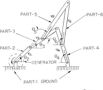
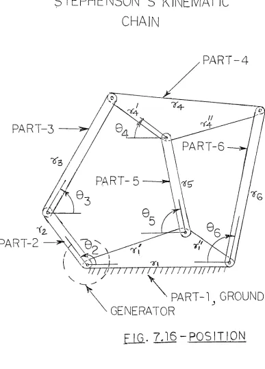
III. DESCRIPTION OF MECHANISM

The linkage mechanism presented in this _study consists

of six links and is a closed

loop

type mechanism. See

figure 1. These six links form two loops. Each

loop

has

four links. Figure 2 describes these loops with their

assumed direction for the analysis. This mechanism has two

types of links. Link 3 is a rigid link with a 120 degree

angle between the two arms while the other links are of the

straight rigid type. The intersection of link 3 and link 6

is a point whose motion is noncircular. Figure 1 describes

the initial position of each link. The clockwise rotation

of crank 2 generates the input motion for the respective

links in the mechanism. The rest of the links have

counterclockwise rotational motion. All angles and angular

velocities measured in the counterclockwise direction are

considered positive.

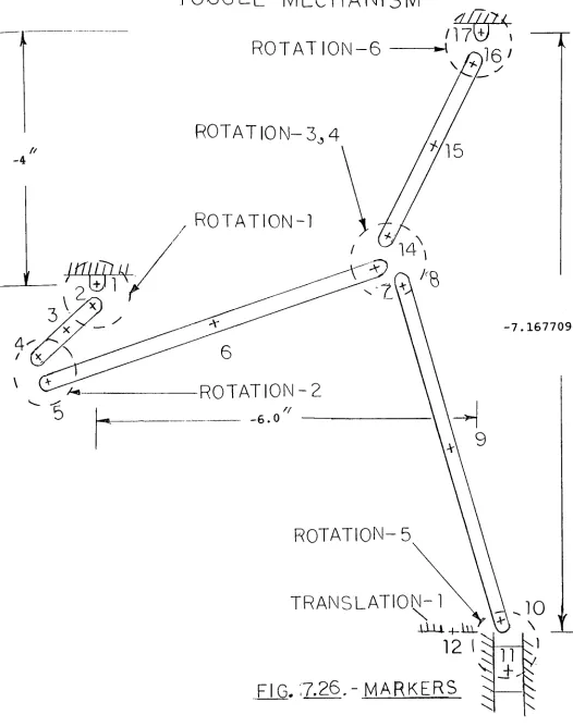
IV- COORDINATE SYSTEM

The analysis of this mechanism employs a right handed

coordinate system. For DRAM analyses, two types of

coordinate systems need to be used. The first coordinate

system is called the local reference axis _system, and

describes the orientation of the link and the positions of

the markers in the link. The orientation of the local

U

CO

W

O

M IH CJ w cu

to

W

CO

o

cj

B

s o

CO

o cu

CO

CJ

^

Q

S3

M

d

M

i>

g

CO

CO >* CO

W

%

M

P

o o CJ

CO

e

CO H

u

tn

O

system. The global coordinate axis system is always

attached to the fixed points of the mechanism. In the

analytical _solution, a simple right hand coordinate system

has been used. Figure 2 and figure 3 show the selected

coordinate systems for the analysis of the mechanism.

V- SELECTED INPUT DATA FOR DYNAMIC ANALYSIS

The

following

input data has been used in the analysis

of the linkage mechanism:

Note that the link of lengths must be referred to the

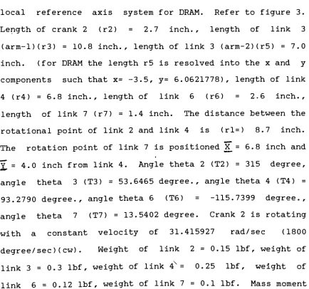
local reference axis system for DRAM. Refer to figure 3.

Length of crank 2 (r2) = _2.7

inch.,

_{length of link 3}

(arm-l)(r3) = _10.8

inch.,

_{length of link 3 (arm-2)(r5)} = _7.0

inch. (for DRAM the length r5 is resolved into the x and _y

components such that x=

-3.5, y=

6.0621778),

length of link 4 (r4) = _6.8

inch.,

length of link 6 (r6) = _2.6

inch.,

length of link 7 (r7) = _{1.4 inch. The} distance between the

rotational point of link 2 and link 4 is (rl=) 8.7 inch.

The rotation point of link 7 is positioned

X_

= _{6.8 inch and}

= _{4.0 inch} from link 4. Angle theta 2 (T2) = 315

degree,

angle theta 3 (T3) = 53.6465

degree.,

angle theta 4 (T4) = 93.2790

degree.,

angle theta 6 (T6) = _-115.7399

degree.,

angle theta 7 (T7) = 13.5402 degree. Crank 2 is rotating

with a constant velocity of 31.415927 rad/sec (1800

degree/sec) (cw) . Weight of link 2

= _{0.15 lbf}

, weight of

link 3 = _0.3

lbf,

weight of link

4X

= _0.25

lbf,

_{weight of} [image:21.551.62.496.278.684.2]

of inertia of link 2 = _{0.00094409 lbf inch.}

sec. sq, mass moment of inertia of link 3 = _{0.02437009 lbf inch. sec.}

sq, mass moment of inertia of link 4 = _{0.00998037 lbf inch.} sec. _sq, mass moment of inertia of link 6 = _{0.00072108 lbf} inch. sec. _sq, mass moment of inertia of link 7 =

0.00018612 lbf inch. sec. sq. Note: Since DRAM

automatically divides the values input for mass and mass moment of inertia

by

gc, the values of mass and mass moment

of inertia used in the DRAM input data _coding need be input in lbm units.

VI. MATHEMATICAL EQUATIONS OF THE ANALYSIS

Since the DRAM results obtained needed to be checked

by

generating an analytical solution, the complex variable method was adopted for the analysis.

However,

the same analysis can be done

by

using the vector method as well. These methods have been explained in "Kinematics And

Dynamics of

Machines"

by Martin,

G. H. To implement the

complex variable method, the linkage mechanism was

considered in two loops. Figure 2 shows the two loops of the mechanism _along with the vector direction of each link

in the respective loop.

The displacement, velocity and acceleration equations

are summarized here and the complete derivation of these

Displacement :

^0-CO

S

a

4-Yg

6053

-^4

COS^

=Y)

CO

Velocity

:

T2.(-Sin(92.)^2.^esin(S33c53--r4C-5^<&4)e^

-o

---C5;

facco52.)(92-i-?3(cosa3)e3

-?^

co)se^)e^-o

C4)

Acceleration:

T2(-Case>;0

Ca.D%^C-

O^c^X^sf

-K3

C~Si'<n3J)c%

^C-sm

2.)

O^V^s

(-Sin

3)

(%)V(3

Ceases

)

93

Second loop:

Displacement:

^Co5^i

+

7sC0is

Vricjass+^ccr.s7=":?&

o*-

--C7^

Velocity: . _

+

Ty

C-S\n7)

C71

-o -

--_

--

--Cc0

vr7

cos

&y

C

Bv)

= o l _

_ ~

,----Oo.)

tV-

os

^; c^

V*

c-sm

er)^+T7c-_o

ez> coyft ^^e7;

e7

=

?4(-Si

n

4)^^7-1

CcoS4)

4^^-Sin<95)C%Vt5CCo3r35)g^

- -" f 1o "\

02-)

The virtual work method has been used to find the

here and the complete analysis of the virtual work is given

in appendix A.

4-[>,

+rrv7

Cf7/a3aJ

&7

7

4^2.^ K^3+Yr^

^

x3

+

<m3^^3

+"^4*4

+

(WH-W^/*s^mfycy6

4^7*7

(.13)

A FORTRAN computer program was written to compute the

angular

displacement,

_velocity, and acceleration of the

various links for a complete cycle of motion. The torque

required at link 2 to drive the linkage through one complete

VII. RESULTS AND DISCUSSION

Computer Graphics:

Schematic drawings of the linkage mechanism have been

generated

by

_{DRAM's postprocessor on the Tektronix terminal.}

DRAM's _ability to save the graphic information

during

a

simulation, for subsequent analysis, is

being

utilized

by

means of the GRSAVE option in the input data coding. The

computer graphics of the linkage mechanism was developed

by

writing a graphics program package in the input data coding.

The various graphics statements used in the graphics program

are explained in the examples of chapter 9 of " A simplified

version of the DRAM user manual " in appendix C. Various

commands have been used to

display

the computer graphics of

the linkage mechanism on the Tektronix terminal. These

commands are summarized in chapter 8 of " A simplified

version of the DRAM user manual ".

Figure 4 shows a hard _copy of the computer graphics of

the mechanism that was obtained. Link 6 and link 7 of the

mechanism are of interest

during

the analysis.

Therefore,

to

identify

the displacement of link 6 and link

7,

an

arrangement of the small circles have been made through the

graphics program at each respective link. The displacements

of other links could be identified in a similar manner.

Kinematics:

Since the linkage mechanism is of closed

loop type,

the

CO CJ

o u 1

tn

a-a

U>

>-*

5

' _o

t> M

1- tu

?

etc. in the program was detected _easily due to DRAM's

ability to correct the initial input data. As result, the

input data was _checked, and corrected.

A complete _description of the linkage mechanism was

input to DRAM through the input data coding language. As

mentioned _earlier, link 6 and link 7 are of interest in this

analysis. Their

displacements,

velocities and accelerations

were determined

by

_requesting these outputs in the DRAM

request statements. Since the step size in the output

statement of the input data coding is

50,

the complete cycle

analysis of the mechanism provides 50 values of each output

request. The time interval of two consecutive output values

is 0.004 second.

However,

the number of output values of

each output request could be increased

by

increasing

the

steps. The values of all angles were output in degrees.

They

can be output in radians

by

_using the RANGLE option in

the output statement.

In order to check the DRAM results, an analytical

solution was done with the

help

of a computer program. The

calculated analytical results show a close match with the

DRAM results. Further more, plots of DRAM results as well

as plots of the analytical results

by

the DIS8 _plotting

software appear to be the same.

Figure 5 though figure 16 show the plots of the DRAM

results and the analytical results. A comparison of figure

5 with figure 6 shows that the nature of these curves

. .,_.

1 1 1 1 1 1 1 1 1 1 1 1 1 1 1 1

%

<B

8> Z

ZJ-2

->--11

s s

in

>-~

0. r o u

in

6

M

a UJ

E-h

LJ

LJ

O

CE

CO

i i

a

or

en

CD

cc

oo

>

LJ

H_I

E-h

CD

u

H

EH

rt5

'J3

2; H Pu a

EH

U

a.

0

o

H

00s

:z:

LJ

LJ

O

en

co

Q

en

_j

ZD

CD

-en

co

>

LJ

E-_J

00y

00

002

00 T

0

p

r^

M

(J

O

Eh

u CJ < Cu CO

M

Q

tJ

O

o

o a CM - O

^-^^

m t>s

^

_ 1 hi

E-h - a

<

u H

LJ

i >

^1

YZ

-LD

2

<4 1

LJ

_ r ₁

^

CJ

- o

r--az

_j ld

a_

-CM _ x-t iJ

CO

CD

L\ - a

O

O

\

_N^

-o

CO

H

en

\1

\. u

CO

yZ.

\

- o

LjJ

_j

1 1

\

z:

_CO

] \ . i M

ZD

\

LT> t Q

CD

\

-l\

3

z

\

az

\

- _{t_j}

^

i

CO

>

\

LJ

\

.

M

ZI

\

Lf>

i i

\

-CM

E

\

\

- a

\

"

o

1 - a

1

o

1

CD

OOt

00

00S

001

0

?!

t

5

1 1 1 1 1 1 1 1 1 1 1 1

X

s

2

s

3?

Xl-I-i

o

UJ

3-uj

S3

H

^

In O

J"

H M u o

UJ J

-IN *^

u.

|-_ _iJ

-i _lo

o a

(0

%

X

_,

WUI

t-> Oi

o M

8"

U.

z

OI

X

KVUJ

io

o<x

o UJ K

xuiuj

a. E O u

Q

O M tn

a ui IE

?

!

-^\

\

V

1 1 1 1 1 1 1 1

1

1 1 1 1 1 1 1

*

s

s

3 (A X UI 0.L) >-vu a_i ro oz >u>

s

I

i

I

o

E-h

az

C

LJ

LJ

o

o

az

C

az

CD

az

co

>

LJ

zz

. i E-h

CD

:*: o o CM LO - o CD LO - O in CM

0000T

V."

|

I 1

oosz

r-T-r-n

ooos

rr

p-n

OOSS

o

o

CO

CD

LjJ

in E< o o LO CD m

f

CM o o o o o I I I I

I

I I I I

I

00SS- 000S-O0SZ-_o p < u H S3 M P U, o s; o H EH $ P W u u p D CJ o M

I

s

IS

XUJUJ o.r

13

i

i

i

I

S5

a.

H P

In

o

O

P

-lot W u u

z

3 < IE

_ fj

-1

5

a

M_ M

W>

P

X

*2o

wo

-in

fc*

r-t USE

<0

a O

H

M

o

E-h

cn

ct:

LJ

O

O

en

cc

LJ

CO

>

LJ

t\

i i i

I

i i i i

I

i i i i

;

i i i i

I

i i i i

|

i i i i

|

000SC 0000C 000SZ 00002

000SI

000OT

000S

g-oas/Ni

NQiiuaanaoou yusNii

o in o

u

H

Eh

S3 l-H

P

tn

O

a

o

p W

u u

<

S3 M

p

r-i

6

M

graph does not agree with the plotted numbers of angular

displacement of link 6 on the _y axis of the analytical

graph. The tabulated numerical output from both solutions

show a close match ( see page 59 and the T6 column on page

71 of appendix B) . It appears that there is a _software

problem in DRAM's _plotting routine. A careful observation

shows that there is a short

delay

in plotting the first

value on the DRAM graph. DRAM draws a straight line from

the origin to this delayed point. This is true for all

plots of DRAM. The angular displacement of link 7 in figure

7 is consistent with the angular displacement of link 7 in

figure 8. In figure 9 the angular _velocity of link 6 is

consistent with the angular velocity of link 6 in figure 10.

The linear velocity values of the plot of link 7 in figure

11 and figure 12 are consisten except near the 0.15 sec.

time area in the DRAM graph. The tabular values of the

linear velocity in this region are _actually negative. In

the DRAM graph the negative values are not plotted on the _y

axis. As a result, the DRAM graph is inconsistent near the

0.15 sec. region. Again

it

appears that there is a

software problem here in DRAM's plotting routine. Figure 13

and figure 14 show the agreement of the angular acceleration

results of link 6.

Finally,

there is also an agreement of

the linear acceleration results of link 7 in figure 15 and

figure 16.

V = _R(W)

(14)

n

An

=

R(W)2-(15)

At

=

K(U)

(16)

AA

=

\[a

+

AZt

(17)

where V is the linear _velocity, R is the length of the

link,

W is the angular _velocity of the

link,

A is the normal

component of _{acceleration,}

A,

is the tangential component of t

acceleration,.^

is the angular _{acceleration,} and A^is the

linear acceleration.

Kinetic:

A schematic

drawing

of the linkage mechanism for the

kinetic analysis is shown in figure 17. Shown here are the

inertia forces and torques associated with each link. Note

that the center of _gravity of link 3 is taken for _simplicity

at the point shown. The vitual work method was used to

determine the torque input at link 2 _necessary to drive the

linkage through one complete cycle. The Newtonian method

can also used for this torque analysis, but the virtual work

method appears to be a simpler approach. The analytical

results for the torque show good agreement with DRAM'S

torque results. Plots of these torque results can be seen

O

Q

W

U <S

o

In

EH

s

S3

H

01

CJ

S3 M P

o

-1

4

1

1 1 1 1 1 1 \T 1 I

1

1 I 1 I I

X

-IN

2

-la.

o

i

?

i

XUJUJ o.E

a

oo-JZ L

M

P

Eh <

OI

o EH

CD

iH

o

CM

E-h

az

LJ

ZD

a

C

o

E-h

o LO o o in -^^^ - o

3

t) * H " in

B

CM p

i

. o

O

cn o

LJ

_S3

H

o

CO

P

. o

UJ

_EH

m

2Z

<

i i

H

in t-H _CH K _i>i _o O H o " o * en r-H in _o o o M In " in ' CM _o - o " o . o a

0*-VIII. SUMMARY

The DRAM software package has proven its usefulness and

effectiveness in the analysis of a complex linkage

mechanism. The DRAM postprocessor has also shown its

importance in computer-aided-design. In short, it was

determined that DRAM is _effectively applicable to solve

mechanical systems of the linkage type. The major findings

of this _study are enumerated below:

1. The computer graphics of the linkage mechanism were

generated

by developing

a graphics program.

Plotting

of

the DRAM results was done

by

_using DRAM's _plotting

commands with the

help

of the Tektronix terminal.

Smoothness of the curves was achieved

by increasing

the

step size in the output statement to

200,

although the

input data _coding shows 50 steps. The step size of 50 is

used to abbreviate the number of output values of the

results.

2. The obtained values of the

displacements,

velocities,

accelerations and torque

by

DRAM compare well with the

analytical results. The results obtained

by

DRAM are,

therefore, consistent with those of the complex variable

method.

A simplified version of the DRAM user manual presents

the second part of the study. In this user _manual, several

examples are presented. The examples are discussed in such

a manner that the reader's

familar^ity

with DRAM is built _up

simplified and made understandable

by

_referring to the

sample examples from time to time. The manual also provides

chapters on _getting started with DRAM and DRAM graphics on

the vax/vms system at the Rochester Institute of Technology.

Finally,

an important

thing

included in the manual is a

chapter on " how to overcome common mistakes and

difficulties which might occur while _running DRAM ".

It was found that there are some difficulties in the

DRAM software. These difficulties can be encountered as

follows:

DRAM does not provide the angular _velocity and

acceleration if the link is rotating about a fixed point.

In such a situation it was necessary to convert the

calculated angular velocity, and acceleration

by

an

analytical method into the linear velocity, and acceleration

respectively for the comparison of results. It is also

noticed

during

this thesis that there is a DRAM software

problem in the plotting routine. DRAM always starts the

plot from the origin regardless of the _starting value. Some

IX.

REFERENCES

1

Vierck,

R. K. ,

Vibration

Analysis

Harper

& Row

Publishers,

Inc,

New

York,

1979.

2

Merian,

J. L. ,

Engineering

Mechanics vol.

2,

Dynamics

John

Wiley

&

Sons,

Inc,

New

York,

Toronto,

1978,

3

Martin,

G. H. ,

Kinematics

And Dynamics of Machines

McGraw-Hill

Book

Company,

New

York,

1969.

4

Hibbleler,

R. C. ,

Encrineerincr

Mechanics,

Dynamics

Macmillan

Publishing

Co.,

Inc,

New York 1983. 5

DiBenedetto,

A.,

"Analysis

_{Of Angular Velocities and}

Accelerations

in Plane Linkages

by

means of Numerical

Procedure",

"Journal of

Mechanisms,

Transmission

and Automation in Design"

vol. 105,1983.

6

Anderson,

R.

A.,

Fundamentals

Of Vibrations

The Macmillan

Company,

New

York,

1967.

7

Church,

A. H. , Mechanical

Vibrations,

Jon

Willey

and

Sons,

Inc,

1967.

8 DRAM user _guide. Dynamic Resoonce Of Articulate

Machinery,

Mechanical Dynamics

Inc,

Ann

Arbor,

Michigan,

Fifth

Edition,

1979.

9

Cheney

W. ; Kincaid D. , Numerical Mathematics

and

Computing

Brooks/Cole

Publishing

Company,

California. Second

Edition,

1985. 10 Beer F. P. , Johnston E. R. , Vector Mechanics For

Engineers,

Fourth

Edition,

McGraw-Hill Book company. New York.

11 DADS

literature,

Dynamic Analysis and Design

System,,

Computer Aided Design

Software,

Inc.

Mathematical Derivations:

Ac shown in fig. ₂ the position vectors for

loop

I can be

written as follows.

1^ Tf3

-YA

~

V,

Separating

real and

imaginary

parts we have

^2

COS

^73 Ccj55

-T0|

L05&4

-

T|

(A-

1

)

T2.

Si

nG>z

-fr^

Si'nG-3

-tZ(

SincS^

-0 -

--(A-2-)

Rearranging

equations (1) and (2)

T3

CO

5

%

=T(

-T2.

C05?_

1^

CO-S-)

Let

__

q

,

-Ti

-rz

Cos

2-^

Cc^tVg

-q| -yYJ\

Cos

(9

4

---(A-3J

tn

3\r^O^

-

bl

r-'M

S'n^|

- - - -

-(

A

-4

J

Squaring

and _adding (3) and ₍₄₎

?/

-qf~-4,

b'trr/f-V

:?-

^l^|

COS

&^

+

Zb|f^,

Sin

e<\

c\\

Cos&~'\

-)-b,Sine.i,

--

f

q' -t-bi

+74

-rjg

)__^A_5)

2?/)

Equation 5 is a transcendental equation in

&

4 . To _solve for

N/q^+tf

S\'n>9

-_bl

a

^f^;

Now equation(5)becomes

\Tq^b?r

0^

Cos9

4-S,n^jSm^)_ -^ItL^Jl^

Let us convert the cosine term into the tangent

by

using

C05-

I

^

\

-j--Loi?"C4-^J

2^>TSI^:

Squaring both sides we get

- _.

C~

1

-b\

-T4 _-t-r3

J

l

+

to^c^-^

^i^ltf)

04

-

tq^

*

1

(^_ci,

_

bi

-T4 _-\-r3

)

Divide equation (2)

by

equation (1)

^"CDse3

qt

h-t^,

GjS^

ta-n

cS3

-

b|

_-y-r^

sms^j

a\

-r-^4

co^-t

Velocity

: Differentiate equations (1) and (2). We get

7aC'SmeOe2

l-r^Cr

Sin

03)3-Y-f

C-^'tdO^

)

^

0

-

-?2Cco53";2

+73

(.co^^e^

-X*,

(Co-s^)

^

=

o

-Rearranging

-r3

^\r)G3e3

-I_-V^i

Sin

<9^

Gz,

-Ta

Si

"n

0Z Bz

^2.

Sm

₀

_^

02

-?/)

Sv

n

^

-fz

O^^

&2

-^A

Co54

-(

A-G)

-CA-7)

6--13

Si'n

e3

f5

0)53

-t*4

os^

^3

Sin

le^-^P

Similarly,

Oq

--73

s

rn

<^3

-^4

S

1n

^

T3

Cos

3

-7^.0*5

9^

^

Sin

Qe3

-4)

Acceleration : Differentiate equations (6) and (7). We have

t?3(-5in3)^-74

C~C0,s4)

Ce^)'-T^

C-S,ne4)^4

"

__--CA-^

4T3

(

cos

0.3

)e3

~*4

(-st*

ne.<o

Cs^2"-^

CCo^o^O^

= o

CA-9)

Rearranging

0- _

Y3

cose3

e3

-7^

co5^

94

e3

-X

J

-4

Cos0-)

N

-nr3Sm3

T'l

Sf'n4

?3

COS

03

-~''4^se-^

^3"^

(

^i2"

Cc6e3

Co$4

-r-Sroe^SmS'^-T-^'C^)

X>

zl"?3T4

sYo^Cosq.,

_-^3^

Cose3

sin

4

=

r3T4

Sin

( 3--|

)

-V-^4

O^lV1-t3

So

C@3

~4)

Similarly,

-rjSVrj3

X

)

r 1

^4

~

~i3

Co5S3

J

f

^

~T3

$i

r>

$3

T4

Sin

64

x>

T4

Sin

C3--1

}

Now the _{position vectors for}

loop

II can be written

as _follows.

The above equation can be written in the complex torm as

f^|

Co54

-*5

Cos

&s

_-VH

Cte&c,

_-Yfj

Cose7

_=v$ Cosy _ - -

(A-\oJ

T4

Si

n^

+

rs-SmS^

Vr6

Sm

&

+r7 Sin6>7

-v<h

sr^^

-

--(A-ll)

Rearranging

7g Cases

^^Co^^j-r^Coso^-r^CasQs

^r7Cose7

Yg

S'o

-^Sin

<p

-t_j

Si'n

&f

-~^5

Sl

'^

$5"

-^7

5i'n

^7

Let

b2

~~

t-^

si n

y

-Y4

Si"n

S4

-ts

Si'n

5

Y6

QJ^Sg

~

q2-?7^7

_____

(A~I2)

Tg

S\nG

-

b2

-T7-Sir,$7

_ . _ . _

(A-13)

By

using the phase angle method we get

-

2-2-2

_^

where

2.

cT

7

Cos-Pi

~-

J_!__

T

W-^.'ti

.2. _, ,2. y

H*2,

^2-ilrv-Vj

, 'bto?_i r

i^bj

a-. ,x, -J

/.

C>xS

C7-0>/)

-

-^-f^+b24-y7

I

f

-nfG

-VU.^

bz

h-t7x

Squaring

both sides we have

\

i ?- . 5L .. V_ /.. 2..

tV "

\

After _simplifying we get

?-__2-\2

+

^l

a

z

-Vy

Cos&y

-q^-r"/

C<?Sv

Velocity

: Differentiate equations ₍₁₀₎ and (11). We get

X^

C-SVrU94)C4)H'V%

[-^0

03)^5

4^

C~5Vn4)(^)

4f7(-Sln(97) C<$>7)

-

0

- - - -

-(A-14)

yA

Cose^

C

<a,

)

4vs

Coses C&s)^

Cos&a

(s)

+-7

Cos/

7)

~o - - - -

(A-/5)

5

-

180

-V

3

4

-1.2 0

-

3

00+^z

0

5

e

3

Rearranging

equations (14) and (15) we gel

-76

s

. o

e

c

c

g

)

~r^7

S(

ezC67

)

~

4-X4

^mai

C^i)

-r-Ts

s,'n

Qs

(3^

-?6

Coo

$C

CQ6^

vrr

to07

C67)

=

A

-T7S110O7

9,

T7

Co^(^7

f$r

'

"" ~~

"-~

-<

^

_T6SinS5 -T7S-n7

cos6

r7C2>se7

OQ~

Av7C0S<97

+8t7Si'o7

-feT7 SrrCG-7)

Similarly,

7

~

-^G

S'/n06

t

^

Coo>

6

-T^SinSG

^

Casc

A

B

-T7Sl'n#7

1_ _

_

13

T^

Si

n

₀

-ATg

COS

9^

Acceleration

:

Differentiate

_equations

(14) and (15). We have

-T4

C-Ces^)C4)2+'^)

C-sm

4

)

&^

4.f^(-Cos .sX^3

4%

(^-Sm

^(5)

^T^

C-Cc^e6)c6s)2'+T6

C~^"n

^<SJ>^

-r^7

C~C(*Se7)

C^7)Xh-T7

C-Si'n7)7

= _O

CA-'^)

- 2_

Y4

C-Si

n

<S^X4jV*4

CC03et^J

04

+rs-C-5i'r)

5J>

CSs)

-VTsrCcos esJ>

as-+rc c-s,,jr>eO

ce^+^CC^eG

;<r

-v77(-S\n-7j)C^73V'T7

Cco^7;e7

~o

CA-17)

Rearranging

Tg

Cr^

n

G6-)

+^7

C-3i

o

G7

) e7

^

-#4

C-

C

06

4)

C

4 )V^

("*

n^4

)

&4

+T^Cas

^C^J

Y6(CO^0^S4-T7

CC0$e7)&7

=

TT4

(-Sin^)

C4)%f^

t

COS

43

6>4

^(-SinGisJKfe)

-H%CC05

65)^5

+T6(-5me^)Ce6^-r-T7

<bS

1^6-7

XzT-

^

Ob

-^

.

s

=

%

e^

-P

T7

3l'r)

tS-7

Qj

-T7

Ga^(P7

?5Sm66

r7sm7

!-*

C3S0&

-^7

eo^o7

_

-pr7

C

os7

-G^

t7

S

i"n

7

"?t7

si'nCD^-?)

Similarly,

< *

B7

=

T

SV"ni9G

T

Sm6

-T

OSG

Y7

s'v n

7

Torque :

The center of mass of each link is shown in figure 17. The

displacement,

velocity, and acceleration of each link are

calculated _{simultaneously} in the

following

mathematical

expressions.

Hence for each link we can write ( Refer to figure 17) :

Link 3 : ,

AS=

T~2_

COS

2L.

as

-^c-sfoe^e^

.

As

-

y^

[>

cos

%^

ce^2"

-t- c-

SJ^J

z.

1

&G{

^7.3Cose3

ti^

=7.3C(-CD5e3i)ce^)2H>C-sin3)>3"]

PR--G

Cos

C<? 0-0.3)

-2-GSm03

PR

=

2-6

C0S693C3)

PR

=

1,C CC-SinGaiC^VGo^^^^

Y33

=

AS

-V

&G\

"V-PR,

(Distance) - - -

C

A-I8J)

73

-as

+s>

-v-Pft

-% (Velocity>

----CA~

'^

yy3

-/AS _-r-Erf? *PR -VI

(Acceleration)-- --C/\-*6)

SS

2-13s

=%[C-sin02)^Sc^^l

<y

OS)

-"7 -3

SiA

e3

Oq

=

7'3C0-S3

3

OP

- Q.

<o

C-^''n3>)^3

tI

j) r-\ i

op

~z^

Cc-coso3;)cp

4-c-siv>e3^3j

7^33

l^jS+

OCD

Op (Distance)

><3

-BS-T-OOf

-OP^Xj

(Velocity)

-X*3

~

B5

_{T-QC]-OPrX;.; (Acceleration)}

~

-(

A-.2

)

_ _

-(A-2.3)

Link 2 :

y2

-Li

COSOi

-' ~

x

y^

=

<ifo CC-

C05

2,)

C<%0

\c->^L)

z]

-- -

C

A

-*0

C

A- 2.4)

(A-2-s)

*2

=

B-Si'n(9z.

- " c^A-2-r)

*2.

~

X%

CCo52j

RETURN

END

KEYWORD DEFINITIONS:

TIME:

Simulation time.

PAR:

Ten parameters.

NGEN:

Identification number of the generator (same as the ID

number of the generator). The NGEN can be used to branch

to the appropriate section of the subroutine when more

than 1 generator is used in the system.

X:

Is the displacement.

DX:

Is the velocity.

D2X:

Is the acceleration.

For Example:

Refer to the Mechanical Dynamics Inc'

s user guide

LINKAGE

MECHANISM C DYNAMIC ANALYSIS D

PART/

1,

GROUND

MARKER/1,GMARKER,PART=1,X=0,Y=0,ANGLE=0 MARKER/

15,

POINT,

PART=1,X=8.

7,

Y=0

MARKER/

14, POINT,

PART=1,X=15.

5,

Y=4.0

PART/2,MASS=0.15,CM=3,INERTIA=0.3645,ANGLE=315 PART / 2,DEGDANGLE=-1800

MARKER/

2, GMARKER,

PART=2,X=0,Y=0,ANGLE=0 MARKER /

3, GMARKER,

PART=

2,

X=_1.3

5,

_Y=0,ANGLE=0

MARKER/4,POINT

,PART=

2,X=2. 7,Y=0

PART/3,MASS=0. 3,CM=19_,INERTIA=9. 4090,ANGLE=233

MARKER/6, POINT,

PART=3,X=0,Y=0

MARKER/ 5,

GMARKER,

PART=3,X=10. 8,Y=0 ,ANGLE=0 MARKER/ 7 ,

POINT,

PART=3,X=-3. 5_,Y=6. 0621778 MARKER/19,

GMARKER,

PART=3,X=3. 5,Y=2. 6,ANGLE=0

PART/4,MASS=0. 25,CM=17,INERTIA=3. 8533,ANGLE=93

MARKER/ 16,GMARKER,PART=4,X=0,Y=0,ANGLE=0 MARKER/ 17 ,

POINT,

PART=4 ,X=3. 4,Y=0

MARKER/18,GMARKER,PART=4,X=6. 8,Y=0,ANGLE=0

PART/6,MASS=0.12,CM=9,INERTIA=0.2784,ANGLE=65

MARKER/

10, POINT,

PART=6,X=0,Y=0

MARKER/9,

GMARKER,

PART=6,X=1 . 3,Y=0,ANGLE=0 MARKER/8,

POINT,

PART=6,X=2. 6_,Y=0

PART/ 7,MASS=0. 1,CM=12,INERTIA=0. 07186,ANGLE=193 MARKER / 1 3,GMARKER,PART=7,X=0,Y=0,ANGLE=0

MARKER/12 ,

POINT,

PART=7,X=0. 7_,Y=0

MARKER/

11, POINT,

PART=7,X=1.

4,

Y=0

ROTATION/1, 1=1,

J=2 ROTATION/

2, 1=4,

J=5 ROTATION/

3, 1=6,

J=18

ROTATION/4, 1=7,

J=8 ROTATION/

5,

1=10,

J=ll ROTATION/

6,

1=14,

J=13 ROTATION/

7,

1=15,

J=16

GENERATOR/

1,

ROTATIONAL, ON=2,CONSTVEL,DEGPAR=-1800,PAR=315. OD

SYSTEM/GC=386.088,JGRAV=-386.088,ERR=1.E-4,IC

OUTPUT /END=0. 2,STEPS=50

,SAVEINT,GRSAVE,NOPLOT

REQUEST/

1,

DISPLACEMENT,

1=9,

J=l REQUEST/

2,

DISPLACEMENT,I=12,J=14

REQUEST/3, VELOCITY, 1=9,

J=l

REQUEST/7,

FORCE,

1=2,

J=l

GRAPHICS

GRAPHICS/1,0UTLINE=2,4

GRAPHICS/ 2,0UTLINE=5,6 GRAPHICS/3,0UTLINE=6,7

GRAPHICS/4,

CIRCLE,

CM=8,RADIUS=0. 1

GRAPHICS/5,0UTLINE=8,10

GRAPHICS/6, CIRCLE,

CM=11,RADIUS=0.05 GRAPHICS/

7,

0UTLINE=

13,

₁₁

GRAPHICS/

8,

0UTLINE=

16,

₁₈

GRAPHICS/9,

CIRCLE,

CM=19

,RADIUS=

. 2

LINKAGE MECHANISM C DYNAMIC ANALYSIS 3

--DEFAULT VALUE (TSM1)

--SYSTEM/TS= _4.0000E-03

SYSTEM HAS 0

DEGREE(S)

OF FREEDOM

SYSTEM WILL BE SIMULATED IN KINEMATIC MODE

* INPUT DATA LOOP CLOSURE CHECK *

j j

I ROTATION 1 DISPLACEMENT I VELOCITY I

I I ERROR I ERROR I

j j j j

I 3 1 9.B7363D-02 I 8. 48230D+01 I I 4 1 2.16149D-01 I 8.48230D+01 I

! j - j

LOOP CLOSURE DISPLACEMENT SOLUTION

CONVERGENCE WITHIN 6.51352D-15 IN 4 ITERATIONS

LOOP CLOSURE VELOCITY SOLUTION

CORRECTED INITIAL CONDITIONS

PART/

PART/ 2

PART/ 3

PART/ 4

PART/ 5

PART/ 6

KFLAG= _{0 ORDER}=

O.0O000000000O0OOD+0O DEG

3.150000000000000D+02 DEG

2.336465358888234D+02 DEG 6.426010474128745D+01 DEG

1.935402462335677D+02 DEG

9.3279025b8285362D+01 DEG

O.OOO0O00O0OOOOOOD+OO RAD/SEC

-3.141592653589793D+01 RAD/SEC

8.194347775570054D+00 RAD/SEC 5.458131723533457D+01 RAD/SEC

B.920737528789960D+00 RAD/SEC

1.933368376638460D+01 RAD/SEC

0 IFCT= ₅₁ H= _0.40000D-02 ITER=

LINKAGE MECHANISM C DYNAMIC ANALYSIS 3

REQUEST NUMBER

MAGNITUDE OF THE LINEAR TIME DISPLACEMENT OF

MARKER 9 RELATIVE TO MARKER 1 0.0000E+OO 1.54806E+01 4.0000E-03 1.52741E+01 8.0000E-03 1.50745E+01 1.2000E-02 1.48857E+01 1.6000E-02 1.47105E+01 2.0000E-02 1.45507E+01 2.4000E-02 1.44077E+01 2.8000E-02 1.42821E+01 3.2000E-02 1.41743E+01 3.6000E-02 1.40B40E+01 4.0000E-02 1.40103E+01 4.4000E-02 1.39525E+01 4.8000E-02 1.39097E+01 5.2000E-02 1.38816E+01 5.6000E-02 1.38682E+01 6.0000E-02 1.38706E+01 6.4000E-02 1.38900E+01 6.8000E-02 1.39285E+01 7.2O00E-02 1.39882E+01 7.6000E-02 1.40714E+01 8.0000E-02 1.41801E+01 8.4000E-02 1.43165E+01 8.8000E-02 1.44821E+01 9.2000E-02 1.46780E+01 9.6000E-02 1.49041E+01 1.0000E-01 1.51581E+01 1.0400E-01 1.54327E+01 1.0800E-01 1.57123E+01 1.1200E-01 1.59703E+01 1.1600E-01 1.61796E+01 1.2000E-01 1.63385E+01 1.2400E-01 1.64770E+01 1.2800E-01 1.66207E+01 1.3200E-01 1.67734E+01 1.3600E-01 1.69289E+01 1.4000E-01 1.70806E+01 1.4400E-01 1.72235E+01 1.4800E-01 1.73548E+01 1.5200E-01 1.74731E+01 1.5600E-01 1.75781E+01 1.6000E-01 1.76680E+01 1.6400E-01 1.77339E+01 1.6800E-01 1.77552E+01 1.7200E-01 1.76978E+01 1.7600E-01 1.751B4E+01 1.8000E-01 1.71780E+01

MAGNITUDE OF THE ANGULAR ANGLE DISPLACEMENT (DEGS) OF

(DEGREES) MARKER 9 RELATIVE TO MARKER 1 1.82315E+01 6.42601E+01 1.87227E+01 7.57727E+01 1.90673E+01 B.57147E+01 1.92413E+01 9.44739E+01 1.92462E+01 1.02283E+02 1.90968E+01 1.09316E+02 1.B8150E+01 1.15721E+02 1.84268E+01 1.21626E+02 1.79594E+01 1.27134E+02 1.74391E+01 1.32317E+02 1.6BB95E+01 1.37210E+02 1.63299E+01 1.41B22E+02 1.57745E+01 1.46132E+02 1.5232BE+01 1.50105E+02 1.47101E+01 1.53699E+02 1.42081E+01 1.56874E+02 1.37269E+01 1.59604E+02 1.32656E+01 1.618B7E+02 1.2B240E+01 1.63756E+02 1.24034E+01 1.652B5E+02 1.20073E+01 1.66593E+02 1.16417E+01 1.67B53E+02 1.13162E+01 1.69291E+02 1.10448E+01 1.71200E+02 1.08477E+01 1.73947E+02 1.07527E+01 1.77991E+02 1.07943E+01 1.B3B64E+02 1.10015E+01 1.92070E+02 1.13643E+01 2.02793E+02 1.17B19E+01 2.15363E+02 1.20712E+01 2.28039E+02 1.21075E+01 2.39104E+02 1. 19126E+01 2.48157E+02

1.15707E+01 2.55720E+02 1.11552E+01 2.6237BE+02 1.07202E+01 2.6B510E+02 1.03117E+01 2.74312E+02 9.97605E+00 2.79841E+02 9.76614E+00 2.85032E+02 9.74402E+00 2.89723E+02

9.97829E+00 2. 93745E+02 1.05315E+01 2.97139E+02

1.143B2E+01 3.00428E+02

1.26825E+01 3.04750E+02

1.41677E+01 3.11852E+02

LINKAGE MECHANISM C DYNAMIC ANALYSIS 3

REQUEST NUMBER

MAGNITUDE OF THE LINEAR

1'IME DISPIjACEMENT of ANGLE

MARKER 12 RELATIVE ( DEGREES)

TO MARKER 14

0. 0000E+00 7. 00000E-01 1. 93540E+02

4. 0000E-03 7. 00000E-01 1. 94787E+02

8. 0000E-03 7. O0O00E-O1 1. 95403E+02

1. 2000E-02 7. 00000E-01 1. 96196E+02

1. 6000E-02 7. 00000E-01 1. 97511E+02

2. 0000E-02 7. OO000E-01 1. 99457E+02

2. 4000E-02 7. 00000E-01 2. 02003E+02

2. 8000E-02 7. 00000E-01 2. 05036E+02

3..2000E-02 7. 00000E-01 2. 0B39BEH-02

3.,6000E-02 7. 00000E-01 2. 11929E+02

4.,0000E-02 7. 00000E-01 2.. 15486E+02

4..4000E-02 7. 00000E-01

n

^i 1B973E+02 4..B000E-02 7. 00000E-01 2. 22347E+02

5..2000E-02 7. OOQOOE-01 2.,25623E+02

5,.6000E-02 7. 00000E-01 -JL.4 28868E+02 6.. 0000E-02 7. 00000E-01 2.,32194E+02

6..4000E-02 7. 00000E-01 2., 35737E+02

6..8000E-02 7. , 00000E-01 2., 39643E+02

7.. 2000E-02 7., 00000E-01 2..44052E+02

7,.6000E-02 7. .00000E-01 2..490BBE+02

8,, 0000E-02 7. , 00000E-01 2..54865E+02

B..4000E-Q2 7. , 00000E-01 2., 61494E+02

8,.8000E-02 7.. 00000E-01

n

.69097E+02 9,.2000E-02 7.. 00000E-01 2,. 77835E+02

9,.6000E-02 7..00000E-01 2., B7911E+02

1,.0000E-01 7,. 00000E-01 2., 99582E+02

1,.0400E-01 7. . 00000E-01 3,. 1310BE+02

1,.0800E-01 7, . 00000E-01 3.. 28586E+02

1,.1200E-01 7.. 00000E-01 3.. 45545E+02

1,.1600E-01 7.. OOOOOE-Ol 2.. 29387E+00

1,.2000E-01 7..00000E-01 1.. 58982E+01

1,.2400E-01 7..00000E-01 2..40943E+01

1,.2800E-01 7..00000E-01 2..70874E+01

1,.3200E-01 7,.00000E-01 2,. 64777E+01

1,.3600E-01 7,.00000E-01 2,. 37437E+01

1,.4000E-01 7,.00000E-01 1.. 99109E+01

1..4400E-01 7,.0OOO0E-01 1,. 57230E+01

1..4800E-01 7,.00000E-01 1,. 1B442E+01 1,.5200E-01 7..00000E-01 9,. 01729E+00

1,.5600E-01 7,.00000E-01 8,. 16242E+00

1..6000E-01 7,.00000E-01 1,. 03435E+01

1..6400E-01 7,.00000E-01 1,

.65245E+01

1..6800E-01 7,.00000E-01 2,. 72947E+01

1,. 7200E-01 7,

.00000E-01 4,. 29356E+01

1,. 7600E-01 7,.00000E-01 6,. 379B4E+01

1..8000E-01 7,.00000E-01 9,. 04911E+01

LINKAGE MECHANISM C DYNAMIC ANALYSIS 3

REQUEST NUMBER

MAGNITUDE OF THE LINEAR MAGNITUDE OF THE ANGULAJ

TIME VELOCITY OF ANGLE VELOCITY (RAD) OF

MARKER 9 RELATIVE

(DEGREES)

MARKER 9 RELATIVE

TO MARKER 1 TO MARKER 1

0.0000E+00 6.37856E+01 _{1.62977E+02 5.45813E+01} 4.0000E-03 5.83049E+01 _1.69650E+02 4.64293E+01 8.0000E-03 5.16218E+01 1.79675E+02 4.05957E+01

1.2000E-02 4.59483E+01 1.92110E+02 3.60060E+01

1.6000E-02 4.22143E+01 2.05833E+02 3.2264BE-t-01

2.0000E-02 4.03800E+01 2.19303E+02 2.92168E+01

2.4000E-02 3.98024E+01 2.31242E+02 2.67725E+01 2.8000E-02 3.97071E+01 2.41159E+02 2.4B360E+01

3.2000E-02 3.95115E+01 2.49184E+02 2.32829E+01

3.6000E-02 3.89079E+01 2.55713E+02 2.19675E+01 4.0000E-02 3.78146E+01 2.61199E+02 2.07437E+-01 4.4000E-02 3.63001E+01 2.66102E+02 1.94856E+01

4.8000E-02 3.45214E+01 2.70B93E+02 1.81013E+01

5.2000E-02 3.26875E-f-01 2.76063E+02 1.65394E+01 5.6000E-02 3.10434E+01 2.820B6E+02 1.47914E+01

6.0000E-02 2.98644E+01 2.89311E+02 1.28933E+01

6.4000E-02 2.94388E+01 2.97B00E+02 1.09277E+01

6.8000E-02 3.00209E+01 3.07198E+02 9.02194E+00

7.2000E-02 3.17632E+01 3.16B21E+02 7.34267E+00

7.6000E-02 3.46755E+01 3.25981E+02 6.0S426E+00

8.0000E-02 3.86454E+01 3.34288E-I-02 5.45953E+00

8.4000E-02 4.34923E+01 3.41706E+02 5.69897E+00

8.8000E-02 4.9006BE+01 3.48460E+02 7.06224E+00 9.2000E-02 5.49470E+01 3.54922E+02 9.85744E+00 9.6000E-02 6.09B15E+01 1.55964E+00 1.44521E+01 1.0000E-01 6.65543E+01 B.89479E+00 2.12325E+01 1.0400E-01 7.06337E+01 1.74285E+01 3.04010E+01 1.0800E-01 7.13590E+01 2.73291E+01 4.13B92E-I-01 1.1200E-01 6.59B51E+01 3.74530E+01 5.17357E+01 1.1600E-01 5.27931E+01 4.27B77E+01 5.65986E+01 1.2000E-01 3.76899E+01 3.09005E+01 5.26393E+01

1.2400E-01 3.53411E+01 1.. 30639E+00 4.36866EH-01

1.2800E-01 4.24780E+01 3~.43073E+02 3.576S6E+01

1.3200E-01 4.81478E+01 3.35325E+02 3.06692E+01

1.3600E-01 5.01821E+01 3.31534E+02 2.77023E+01

1.4000E-01 4.89070E+01 3.29869E+02 2.59504E+01

1.4400E-01 4.46838E+01 3.30560E+02 2.47242E+01

1.4800E-01 3.78293E+01 3.35567E+02 2.34733E+01 1.5200E-01 2.95685E+01 3.50631E+02 2.17033E+01

1.5600E-01 2.55835E+01 2.62070E+01 1.90992E+01

1.6000E-01 3.5B0S1E+01 6.59223E+01 1.60061E+01

1.6400E-01 5.75816E+01 8.B4510E+01 1.39807E-I-01

1.6800E-01 8.399B2E+01 1.033B7E+02 1.55543E+01

1.7200E-01 1.10829E+02 1.17152E+02 2.3427BE+01

1.7600E-01 1.34118E+02 1.32573E+02 4.02678E+01

LINKAGE MECHANISM C DYNAMIC ANALYSIS 3

REQUEST NUMBER

MAGNITUDE OF THE LINEAR

I"IME VELCICITY OF ANGLE MARKER 11 RELATIVE ( DEGREES )

TO MARKER 1

0. 0000E+00 1. 24B90E+01 2. B3540E-1-02 4.0000E-₀₃

4. 50840E+00 2. 84787E+02 8.

0000E-03 3. 78699E+00 2. 85403E+02 1.

2000E-02 6. 23563E+00 2. 86196E+02 1.

6000E-02 9. 93223E+00 2. 87511E-I-02 2.

0000E-02 1. 3B022E+01 2..B9457E+02

2.4000E-_{02 1.71849E+01 2.}

,92003E+02

2..

8000E-02 1. 97024E+01 2.,95036E+02

3.

2000E-02 2. 12128E+01 n

,9B39BE+02

3.

6000E-02 2. 17726E+01 3., 01929E+02

4.,

0000E--02 2. 15B97E+01 3.. 054B6E+02

4. -02 2. 09704E+01 3., 08973E+02

4.,

8000E-02 2.,02661E+01 3.. 12347E+02

5..

2000E--02 1. 98237E+01 3.. 15623E+02

5. -02 1.,99412E+01 3.. 18B6BE+02

6.,

0000E--02 2., 08319E+01 3.. 22194E+02

6. -02 2..26035E+01 3.. 25737E+02

6..

8000E- _{02 2.}

, 52594E+01 3..29643E+02

7. -02 2.. 872B6E+01 3.. 34051E+02

7, -02 3., 29184E+01 3.. 39088E+02

8..

0000E--02 3., 77747E+01 3..44865E+02

8. -02 4., 33297E+01 3..51494E+02

8. -02 4..97282E+01 3..59098E+02

9,.

2000E--02 5.. 72261E+01 7..B3470E+00

9, -02 6..61459E+01 1.. 79113E+01

1,. 0000E--01 7,.67225E+01 2,. 95B24E+01

1,. 0400E--01 a.. B6597E+01 4,.31075E+01 1,.

0800E--01 1.. 00041E+02 5.. 85B61E+01

1..

1200E--01 1.. 05469E+02 7.. 55453E+01

1,.

1600E--01 9,. 59417E+01 9,. 22939EH-01

1,.

2000E--01 6,. 77000E+01 1..05B98E+02 1, -01 3.. 28281E+01 1,. 14094E+02

1,.

2B00E--01 5,.54113E+00 1.. 170S7E+02

1, -01 1.. 14689E+01 2,. 96478E+02

1,.

3600E--01 2,.09121E+01 2,.93744E+02

1. -01 2,.51779E+01 2.. B9911E+02

1. -01 2..53271E+01 2..85723E+02

1, -01 2,. 13163E+01 2..81B44E+02

1, -01 1.. 22327E+01 2.. 79017E+02

1. -01 2,. 94869E+00 9,. B1624E+01

1, -01 2,.47154E+01 1,. 00343E+02

1, -01 5,. 13927E+01 1,. 06525E+02

1. -01 8,. 04302E+01 1,

. 17295E+02

1,.

7200E--01 1,. 10987E+02 1,.32936E+02

1..

7600E--01 1,. 44585E+02 1,

. 5379BE+02

1..

8000E--01 1,. 81802E+02 1,

. 80491E+02

1. -01 2,. 09496E+02 2,. 12876E+02

1.

LINKAGE MECHANISM C DYNAMIC ANALYSIS 3

REQUEST NUMBER

MAGNITUDE OF THE LINEAR TIME _{ACCELERATION OF}

MARKER 9 RELATIVE

TO MARKER 1

0.0000E+OO 1.54301E+03 4.0000E-03 2.72731E+03 8.0000E-03 3.02351E+03 1.2000E-02 2.92359E+03 1.6000E-02 2.64141E+03 2.0000E-02 2.2B099E+03 2.4000E-02 1.90161E+03 2.8000E-02 1.54491E+03 3.2000E-02 1.24517E+03 3.6000E-02 1.02913E+03 4.0000E-02 9.06964E+02 4.4000E-02 8.63684E+02 4.8000E-02 8. 70063E+02

5.2000E-02 9.05031E+02 5.6000E-02 9.634B3E+02 6.0000E-02 1.04856E+03 6.4000E-02 1.16102E+03 6.8000E-02 1.29464E+03 7.2000E-02 1.43B94E+03 7.6000E-02 1.5B457E+03 8.0000E-02 1.72675E+03 8.4000E-02 1.86624E+03 8.8000E-02 2.00909E+03 9.2000E-02 2.166B2E+03 9.6000E-02 2.35825E+03 1.0000E-01 2.60946E+03 1.0400E-01 2.93473E+03 1.0800E-01 3.27097E+03 1.1200E-01 3.50518E+03 1.1600E-01 4.06133E+03 1.2000E-01 4.88433E+03 1.2400E-01 4.29041E+03 1.2800E-01 2.78257E+03 1.3200E-01 1.45516E+03 1.3600E-01 5.83362E+02 1.4000E-01 7.11773E+02 1.4400E-01 1.47442E+03 1.4800E-01 2.43709E+03 1.5200E-01 3.63056E+03 1.5600E-01 5.02876E+03 1.6000E-01 6.43046E+03 1.6400E-01 7.57507E+03 1.6800E-01 8.46487E+03 1.7200E-01 9.43317E+03 1.7600E-01 1.10896E+04 1.8000E-01 1.39143E+04

MAGNITUDE OF THE ANGULAR

ANGLE ACCELERATION (RADS) OF

(DEGREES)

MARKER 9 RELATIVE

TO MARKER 1

2.902B3E+02 -2. 50598E+03

2.96738E+02

-1. 67960E+03

3.01779E+02 -1. 27776E+03

3.06176E+02 -1. 03198E+03

3.10706E+02 -8.44429E+02

3.16055E+02 -6.83023E+02 3.22878E+02 -5. 43037E+02

3.31823E+02 -4. 30429E+02

3.43441E+02 -3. 52293E+02

3.57626E+02 -3. 11577E+02 1.26094E+01 -3.0561BE+02 2.51593E+01 -3.27290E+02 3.2B951E+01 -3.67021E+02 3.55619E+01 -4.14303E+02 3.43392E+01 -4. 58213E+02 3.09994E+01 -4. 87363E+02 2.72807E+01 -4.90131E+02

2.43866E+01 -4. 55743E+02 2.28598EH-01 -3.7574BE+02

2.2B161E+01 -2.445B4E+02 2.42673E+01 -5.B2284E+01 2.73656E+01 1. B8681E+02 3.25491E+01 5.05723E+02

4.06061E+01 9.07301E+02

5.26460E+01 1.