Performance Analysis of Stiction Detection Methods

(1)



Abstract: Industrial studies stated that, nearly 30% of badly performing process control loops are produced by nonlinearities in the pneumatic control valves, one among the main cause is stiction. The influence of this stiction nonlinearity is commonly detected as the process variable oscillations. As industrial plants contain several loops that are interacting, these oscillations will be spread to the whole system. Overhauling the defective valves will be the one among the top solution to this problem, which is probable only during the period of shut down process. But, this solution of process shut down to separate the defective valve is not cost-effective solution and hence it is taken into account as the prime one. So, there is a necessity for a technique to identify the effect of the control valve stiction. Detection algorithms available in literature are numerous and these techniques create either a quantitative or a qualitative statement about the occurrence of stiction in the control valve. While using available data, a detection method is considered to be effective only when its concluding result is relatively reliable. The main drawback while detecting stiction is that the stem position (MV) of the valve is not available in most of the situations. Quantifying the actual position of the control valve stem is always not probable. Commonly, process output and controller output are taken as the available data from most of the processes. The methods which use these data sets (PV and OP) are more appreciable by the control engineers. In this work, modified bispectral analysis technique is used as control valve stiction detection method and to prove its efficiency four different existing detection techniques available in literature are considered in this study and the performance of each method is reported. Here, eleven different data sets, seven from different laboratory processes and four from process industries are used to make the comparative analysis of performance.

Keywords: Detection, stiction, stem position, process output, controller output, Modified Bispectral analysis.

I. INTRODUCTION

Hundreds to thousands of process control loops is comprised in a typical chemical plant. The deviances from desired values has diverse root causes in which external disturbance, improper controller tuning and nonlinearities in the system are some of the known causes of bad performance [1].

Pneumatic control valves are common instruments in industrial settings and the resistance offered from the stem packing is often considered as the main cause of stiction.

Revised Manuscript Received on September 03, 2019

.Abirami, Research Scholar, Department of Electronics and

Instrumentation Engineering, Annamalai University, Chidambaram - 608002, India.

S.Sivagamasundari, Department of Electronics and Instrumentation

Engineering, Annamalai University, Chidambaram - 608002, India

.

Generally, a valve in good state of maintenance presents low stiction; though, over time, this nonlinearity has a tendency to increase. The existence of stiction declines the control loop efficiency and even causes oscillations in the controlled variable. Despite being the best solution, at times removing the valve for maintenance purpose is not possible. So, particularly when maintenance is not accessible, there is a requirement for a technique to detect and diagnose the consequence of the stiction in the control valve [2].

A. Detection Methods Considered For Analysis

In order to prove the efficiency of the modified bispectral analysis technique, four different existing detection techniques available in literature are considered in this study and the performance of each method is reported. The detection techniques considered for analysis are,

(1) Cross Correlation Method (CCM) - This method by Horch et al., uses PV and OP data to predict the occurrence of stiction in a process control system [3].

(2) Curve Fitting Method (CFM) - The idea of this method proposed by He et al. is based on fitting of PV data to a triangular wave or a sinusoidal wave [4].

(3) Relay Based Method (RBM) - Rossi and Scali, proposed this method which is based on the likeness of shapes of the process variable amongst the loops affected by control valve stiction and loops under the relay control [5].

(4) Area Calculation Method (ACM) - The key idea of this method proposed by Salsbury et al. is to extract features of the process variable between zero-crossing events [6].

II. LABORATORYCONTROLLOOPSFOR

STUDY

The following three laboratory process control loops are deliberated for the study.

A. Airflow Process

The Airflow process under consideration shown in Figure 1, consists of accessories like blower, cold air circulation line with manual control valves, bypass valve, pneumatically operated control valve, orifice fitted in the pipe line to produce differential pressure for the rate of flow of air.

S.Abirami, Research Scholar, S.Sivagamasundari,

(2)

[image:2.595.57.275.51.202.2]

Fig. 1 Laboratory Airflow Process

Three closed loop data sets are taken from the laboratory airflow process.

(i)The first set of data is obtained by introducing stiction (by tightening the stem pack screws) in the control valve. (ii) The second set is due to external disturbance (introduced by continuous opening and closing of by-pass valve). (iii) The third set of data is the result of Aggressive controller tuning.

The PV and OP data sets from airflow process used for various detection techniques are presented in Figures 2 to 4.

650 700 750 800 490 492 494 496 498 500 502 504 506 508 510

Time (Sampling instants)

Fl ow r at e (lp m ) SP PV

650 700 750 800 5 5.5 6 6.5 7 7.5

C on tr ol le r ou tp ut ( m A )

(a) Process Variable (b) Controller output

Fig. 2 Data set of Airflow process with Valve Stiction

150 200 250 300 350 485 490 495 500 505 510 515 520 Time (sec) Fl ow r at e (lp m )

150 200 250 300 350 4 5 6 7 8 9 10 Time (sec) C on tr ol le r ou tp ut ( m A )

[image:2.595.316.538.158.312.2]

Fig. 3 Data set of Airflow Process due to External Disturbance

150 200 250 300 350 496 498 500 502 504 506 508

150 200 250 300 350 4 6 8 10 12 14 16 18 20 C on tr ol le r ou tp ut ( m A )

Fig. 4 Data set of Airflow Process due to Aggressive Controller Tuning

B. Level Control of Spherical Tank Process

A real time experimental setup for a nonlinear spherical tank is presented in Figure 5. This consists of a spherical tank, pump, a water reservoir, Rotameter, an electro pneumatic converter (I/P converter), a Differential Pressure Transmitter (DPT) and a pneumatic control valve. From the water reservoir, the air failure to close type pneumatic control valve

regulates the flow of the water pumped to the spherical tank. The water level in the tank measured by the DPT and is transmitted (4-20 mA) to the interfacing module and then to the PC. Control signal is transmitted from I/P converter (4-20 mA), after computing the control algorithm in the PC, so that the pressure actuates the pneumatic control valve. By this the required flow of water is produced in and out of the tank. Thus a continuous flow of water in and out of the tank is maintained.

Fig. 5 Experimental Setup of Laboratory Spherical Tank Level Process

Two closed loop data sets are taken from the spherical tank level process.

(i)The first set is due to external disturbance (introduced by continuous opening and closing of solenoid valve).

(ii) The second set of data is the result of aggressive controller tuning (by increasing the integral time).

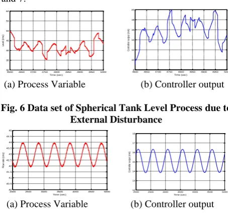
The PV and OP data sets from spherical tank level process used for various detection techniques are presented in Figures 6 and 7.

4600 4650 4700 4750 4800 4850 4900 4950 5000 30 35 40 45 50 55 60 Time (sec) Le ve l ( cm s)

46008 4650 4700 4750 4800 4850 4900 4950 5000 10 12 14 16 18 20 Time (sec) C on tr ol le r ou tp ut ( m A )

[image:2.595.53.282.327.408.2]

Fig. 6 Data set of Spherical Tank Level Processdue to External Disturbance

2000 2500 3000 3500 4000 4500 5000 40 40.5 41 41.5 42 42.5 43 43.5 44 44.5 45 Time (sec) Fl ow r at e (c m s)

2000 2500 3000 3500 4000 4500 5000 12 13 14 15 16 17 18 Time (sec) C on tr ol le r ou tp ut ( m A )

[image:2.595.311.538.434.649.2]

Fig. 7 Data set of Spherical Tank Processdue to Aggressive Controller Tuning

C. Pressure Process

The experimental setup for the laboratory pressure process is presented in Figure 8. The process variable (pressure) is sensed by a piezo electric pressure transmitter, which produces current output in the 4 to 20 mA range. The PI controller is tuned using ZN method. The air failure to open (AFO) pneumatic control valve

[image:2.595.55.278.446.532.2]

(3)

[image:3.595.310.543.53.226.2]

the process pipeline, thus controlling the pressure.

Fig. 8 Laboratory Pressure Process

Two test cases are considered for the pressure control process.

(i)The loop is excited by simultaneously applying a set point change at time zero and introducing a Gaussian noise disturbance of 0.001% variance. The External disturbance is applied by opening and closing of the by-pass valve. (i)The integral time is increased by 10%, hence the

occurrence of comparatively produces large oscillations in the process variables due to large integral action.

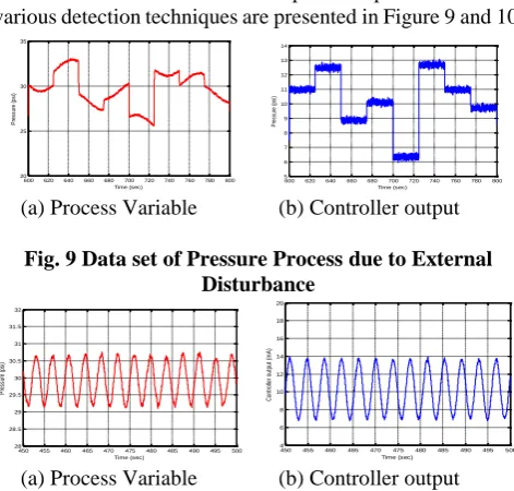
The PV and OP data sets from pressure process used for various detection techniques are presented in Figure 9 and 10.

600 620 640 660 680 700 720 740 760 780 800 20 25 30 35 Time (sec) P re ss ur e (p si )

600 620 640 660 680 700 720 740 760 780 800 5 6 7 8 9 10 11 12 13 14 Time (sec) P re ss ur e (p si )

Fig. 9 Data set of Pressure Processdue to External Disturbance

450 455 460 465 470 475 480 485 490 495 500 28 28.5 29 29.5 30 30.5 31 31.5 32 Time (sec) P re ss ur e (p si )

450 455 460 465 470 475 480 485 490 495 500 4 6 8 10 12 14 16 18 20 Time (sec) C on tr ol le r ou tp ut ( m A )

[image:3.595.305.542.54.417.2]

Fig. 10 Data set of Pressure Processdue to Aggressive Controller Tuning

D.Data Sets from various Industrial Processes To substantiate the claim that the proposed detection method is very effective, data recorded from four industrial control loops which includes flow control (FC), level control (LC), temperature control (TC), and pressure control (PC) systems are also used and the results are analyzed. Here, all loops are known to be affected by stiction nonlinearity. Recorded response of controller output (OP) and process variable (PV) are demonstrated in Figures 11 and 12.

2000 2100 2200 2300 2400 2500 2600 2700 2800 2900 3000 30

35 40 45 50

Fl o w r a t e ( % )

2000 2100 2200 2300 2400 2500 2600 2700 2800 2900 3000 70

80 90 100

Te m p e r a t u r e ( d e g C )

(a) Industrial Flow (b) Industrial Temperature Process Data Process Data

2000 2100 2200 2300 2400 2500 2600 2700 2800 2900 3000 20

22 24

Time (sampling instants)

L e v e l ( c m s )

1000 1050 1100 1150 1200 1250 1300 1350 1400 1450 1500 60

65 70

P re s s u re ( % )

[image:3.595.64.276.70.234.2]

(c) Industrial Level (d) Industrial Pressure Process Data Process Data

Fig.11 Recorded Values of Process Variable for Four Industrial Loops in the Presence of Stiction

2000 2100 2200 2300 2400 2500 2600 2700 2800 2900 3000 30

35 40 45 50

Fl o w r a te ( % )

20002100 220023002400 2500 260027002800 2900 3000 70

80 90 100

Te m p e ra tu re ( d e g C )

(a) Industrial Flow (b) Industrial Temperature Process Data Process Data

2000 2100 2200 2300 2400 2500 2600 2700 2800 2900 30000 5

10

Time (Sampling instants

C o n tr o ll e r o u tp u t (V o lt s )

1000 1050 1100 1150 1200 1250 1300 1350 1400 1450 1500 58 60 62 64 66 68

C o n tr o ll e r o u tp u t (% )

(c) Industrial Level (d) Industrial Pressure Process Data Process Data

Fig. 12 Recorded Values of Controller output for the Four Industrial Loops in the Occurrence of Stiction

III. DETECTIONOFVALVESTICTIONUSING MODIFIEDBISPECTRUM(MBM)

Based on higher order statistics, the modified bispectrum provides a means to identify nonlinearity when oscillations exist in process systems. The detection approach that is based on modified bispectrum can discriminate between the oscillations induced by bad tuning and external disturbances from valve non-linearity induced oscillations, which are the most common reasons for limit cycles in process systems. The purpose of this analysis is to validate the application of HOS-based modified bispectrum techniques in analyzing the causes of poor performance. An easier solution is to normalize the bispectrum to get a new measure whose variance is independent of the signal energy [7]. Similar to the conventional bicoherence, a normalized form of modified bispectrum is, ) 1 . 5 ( ) ( ) ( ) ( ) ( ) ( ) ( ) , ( ) , ( 2 2 1 2 1 2 2 * 2 * 2 2 2 1 2 1 2 f f X f f X E f X f X f X f X E f f B f f b MS MS   

A beneficial feature of the bicoherence function is that it removes the dependency on amplitude and takes on an amplitude value between 0 and 1. Therefore, this function can be used to detect the presence of nonlinearities. If for a given system, the modified bicoherence is closer to zero, it represents the linearity of the

[image:3.595.312.540.270.419.2] [image:3.595.50.286.353.578.2]

(4)

of nonlinearity. In order to enhance the detection procedure, in addition to modified bispectrum, modified bicoherence is also used to detect the valve stiction.

A. Aggressive Controller Tuning

[image:4.595.313.539.52.157.2]

The responses shown in Figures 4, 7 and 9 are typical examples of aggressive controller tuning. Figures 13 to 15 show the results of modified bispectrum. The occurrence of comparatively higher integral action yields bigger oscillations in the process variables

.

Fig. 13 Modified bispectrum map of Airflow Process for Aggressive Controller Tuning (Max.

[image:4.595.54.281.160.278.2]

Bicoherence=0.01487)

Fig. 14 Modified Bispectrum Map of Spherical Tank Level Process for Aggressive controller tuning

[image:4.595.315.538.198.321.2]

(Max. Bicoherence =0.0173)

Fig. 15 Modified Bispectrum Map of Pressure Process for Aggressive Controller Tuning

(Max.Bicoherence = 0.0951)

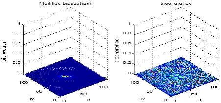
B.Presence of External Oscillatory Disturbance. Figure 3, 6 and 10 shows time trends of PV and OP in the presence of external disturbance. In order to differentiate the oscillations induced by the external disturbances from the stiction induced oscillations, modified bispectrum plot and the corresponding bicoherence plot are obtained and are shown in the Figures 16 to 18.

Fig.16 Modified Bispectrum Map of Airflow Process for External Disturbance(Max: Bicoherence = 0.1925)

Fig. 17 Modified Bispectrum Map of Spherical Tank Level Process for External Disturbance (Max.

Bicoherence = 0.0786)

[image:4.595.49.285.314.627.2]

The tests give the bicoherence of 0.1925, 0.0786 and 0.0927 respectively. These results clearly show that the reason for the oscillation is not due to any nonlinearity in the system. The bicoherence plot is also flat.

Fig.18 Modified Bispectrum Map of Pressure Process for External Disturbance

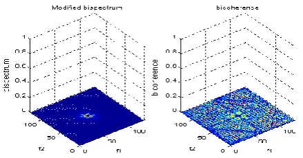
(Max. Bicoherence =0.0927) C. Occurrence of Control Valve Stiction

The modified bispectrum method is then applied to the industrial control loops and the laboratory airflow process data for stiction detection. Figures 2, 11 and 12 depict time trends of the PV and OP.

[image:4.595.315.540.403.526.2] [image:4.595.326.552.618.721.2]

(5)

[image:5.595.303.574.178.349.2]

Figures 19 to 23 show the corresponding modified bispectrum maps exhibiting significant peaks.

[image:5.595.62.266.239.355.2]

Fig. 20 Modified Bispectrum Map of Industrial Flow Process Data (Max. Bicoherence = 0.9284)

[image:5.595.62.278.393.501.2]

Fig. 21 Modified Bispectrum Map of Industrial Temperature Process Data (Max. Bicoherence = 0.97152)

Fig. 22 Modified Bispectrum Map of Industrial Level Process Data (Max. Bicoherence = 0.97581)

Fig. 23 Modified Bispectrum Map of Industrial Pressure Process Data (Max. Bicoherence = 0.9981) From the above results, the maximum bicoherence calculated by modified bispectrum analysis is found to be 0.7049, 0.9284, 0.97152, 0.97581 and 0.9981. The modified bispectrum is also greater than the threshold value (0.01). Hence this ascertains the occurrence of stiction in the control valves involved in all these processes.

IV. RESULTSANDDISCUSSIONS

The detection methods considered for analysis in the above section have been applied to the data sets obtained from the laboratory and industrial control loops. The results with the indication of stiction are given in Table I. (Here the notations used are: Y - Stiction; N - No stiction; U – uncertain).

Table I. Results of Valve Stiction Detection

The following abbreviations are used in the table I.

1.Experimental Airflow process data (Valve stiction) – EXAF1 2.Experimental Airflow process data (Aggressive tuning) – EXAF2 3.Experimental Airflow process data (External disturbance) –EXAF3

4.Experimental Spherical tank level process data (Aggressive tuning) – EXSTL1

5.Experimental Spherical tank level process data(External disturbance) – EXSTL2

6.Experimental Pressure process data (Aggressive tuning) – EXP1 7.Experimental Pressure process data(External disturbance)– EXP2 8.Industrial Flow process – IFP

9.Industrial Temperature process – ITP 10.Industrial Level process – ILP 11.Industrial Pressure process – IPP

From Table I it is inferred that application of cross correlation technique to industrial flow process data, curve fitting method to industrial pressure process data and area peak method to laboratory spherical tank level process data with external disturbance data are not able to predict the occurrence of stiction in control valves of these processes.

V. CONCLUSION

Five different non-linearity testing techniques that help to identify the root causes are considered and their performances are compared. Even though the modified bispectral technique based on higher-order statistics is sensitive to abrupt changes and non-stationary trends, it is found to be more reliable. The detection algorithm based on modified bispectrum has been effectively assessed by applying it to three laboratory and four industrial case studies. In all cases, the algorithm could successfully detect control valves that are suffering from

stiction. It has been shown that the stiction-detection algorithm

Data set

Method

CCM CFM RBM APM MBM

EXAF1 Y Y Y Y Y

EXAF2 N N N N N

EXAF3 N N N N N

EXSTL1 N N N N N

EXSTL2 N N N Y N

EXP1 N N N N N

EXP2 N N N N N

IFP U Y Y Y Y

1TP Y Y Y Y Y

ILP Y Y Y Y Y

[image:5.595.58.278.542.657.2]

(6)

can detect blindly without knowing the type of control valves or type of control loops. The algorithm requires only the set point and process variable data. If the process is oscillating and the cause is due to poorly tuned controllers or due to an external oscillatory disturbance, the proposed method does not detect any nonlinearity. The graphical plots have been found to be beneficial in detecting the causes for bad performance of control loops. The detection of nonlinearity revealed by the significant peak in the bispectrum map confirms the occurrence of stiction in control valve, since the process is considered to be linear around the operating range.

REFERENCES

1. S.Sivagamasundari, D.Sivakumar, “A New Methodology to

Compensate Stiction in Pneumatic Control Valves”, International

Journal of Soft Computing and Engineering, Volume-2, Issue-6, 2013.

2. [2] Bruno C. Silva and Claudio Garcia, “Comparison of Stiction

Compensation Methods Applied to Control Valves”, 53, 3974−3984, 2014.

3. [3] A. Horch, “Oscillation diagnosis in control loops- stiction and other

causes”, Proceedings of the 2006 American Control Conference,

Minneapolis, Minnesota, USA, June 14-16, 2006.

4. [4] Q.P. He, J. Wang, M. Pottmann, and S.J. Qin, “A curve fitting

method for detecting valve stiction in oscillating control loops”,

Journal ofIndustrial and Engineering Chemistry Research, vol.46, pp.4549-4560, 2007.