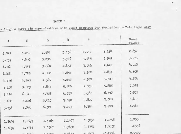
Solutions of the nonlinear diffusion equation : existence, uniqueness, and estimation

;...s

A

,

II

SOLUTIONS OF THE NONLINEAR DIFFUSION EQUATION: EXISTENCE, UNIQUENESS, AND ESTIMATION

by

John Howard Knight

A thesis submitted for the degree of Doctor of Philosophy

at the Australian National University

STATEMENT

Unless it is stated in the text to the contrary, the material contained in this thesis is the product of my own research.

ACKNOWLEDGEMENTS

I would like to thank the Australian National University for the award of a research scholarship, and Dr John Philip and Mrs Masako Izumi for their supervision. In particular I thank Dr Philip for many informative discussions, and constant

ABSTRACT

In the first part of the thesis a problem for the nonlinear

diffusion equation with diffusion coefficient a function of concentration, which is reduced by a similarity substitution to a boundary value

problem for a nonlinear ordinary differential equation, is considered. Existence of a solution with certain upper and lower bounds is

demonstrated for diffusion coefficient satisfying a local Lipschitz condition, and uniqueness is proved for non-increasing diffusion coefficient. An iterative method of Crank and Henry for solving this problem is investigated and is proved to converge for non-decreasing diffusion coefficient, thus extending the existence result in this case. A perturbation method is used to derive a general series solution to the problem for a class of diffusion coefficients of power-law and

exponential form.

More general problems are considered in the last two chapters of the thesis. It is shown that a particular nonlinear diffusion equation with flux boundary conditions can be transformed to a linear equation, and new exact solutions are given to various problems of practical interest involving this nonlinear diffusion equation. An iterative method proposed by Parlange to solve various problems for the nonlinear

diffusion equation and related equations is investigated, and it is shown that the method of Parlange fails to converge. The problems are

TABLE OF CONTENTS

STATEMENT

ACKNOWLEDGEMENTS ABSTRACT

CHAPTER 1 INTRODUCTION

1.0 The equations to be solved 1.1 Exact solutions

1.2 Approximate solutions

CHAPTER 2 EXISTENCE, UNIQUENESS AND PROPERTIES OF SOLUTIONS FOR A TWO POINT BOUNDARY VALUE PROBLEM

2.0 Preliminary results 2.1 Uniqueness results

2.2 Existence and properties of solutions

CHAPTER 3 THE METHOD OF CRANK AND HENRY 3.0 The method

3.1 Preliminaries

3.2 Convergence proof for non-decreasing D

CHAPTER 4 AN ANALYTICAL SOLUTION BY PERTURBATION METHOD 4.0 Application of the Kirchhoff transformation 4.1 The perturbation expansion

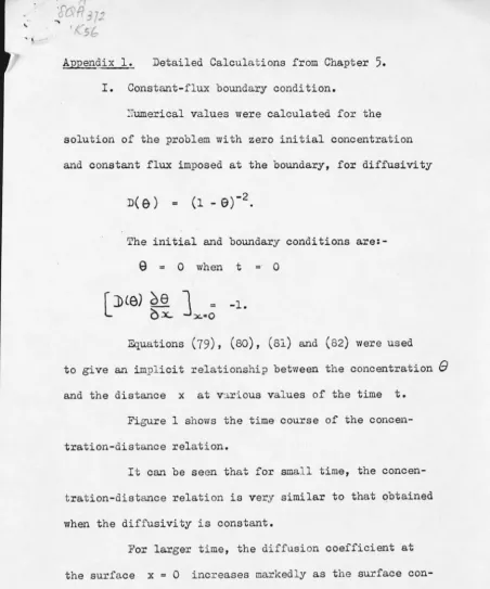
CHAPTER 5 A NEW EXACT SOLUTION FOR A NONLINEAR DIFFUSION EQUATION WITH CONSTANT-FLUX BOUNDARY CONDITION

5.0 The method of Storm

5.1 Application of the method to more general problems 5.2 An exact solution corresponding to an instantaneous

plane source

5.3 The solution to the general problem, and extensions to variable flux

ii i i i iv

1 4 5

10 15 19

28 29 32

38 41

47

54

CHAPTER 6 CRITIQUE AND IMPROVEMENT OF PARLANGE'S ITERATIVE

METHOD

6.1 The problem as an integral equation 6.2 Improvement of the Parlange method

REFERENCES

58 60 63

INTRODUCTION

1.0 THE EQUATIONS TO BE SOLVED

The

mathematical theory of diffusion

ae

at

where the dependent variable 8 is the concentration of diffusing

substance, and Dis the diffusion coefficient, which may be a function of the independent variables and of the dependent variable 8. When D varies with 8, we have the nonlinear diffusion equation.

The

diffusion equation

heat equation

at

where Tis the temperature, and C and k are respectively the heat

capacity and thermal conductivity of the material, which may be functions of the independent variables and of the temperature.

In particular the nonlinear diffusion equation may be applied to the movement of water in soils, when the influence of gravity may be

neglected. When gravity must be taken into account, the process is described by the nonlinear Fokker-Planck equation

ae

at

dK

ae

'i/•(D'i/8)+-•-_d

_{e az}

_,

D may vary through two or three decades, and dK/d6 through several more (Philip, 1969).

In most problems considered here it will be required to find a solution of equation (1) in a semi-infinite one-dimensional region, with certain initial conditions, and subject to boundary conditions of either the concentration type, in which the concentration is specified on the boundary, or of the flux type, in which the flux -D a6/an is specified on the boundary, where Dis the diffusion coefficient, and a6/an denotes differentiation in a direction normal to the boundary. The thermal parameters C and k will be functions of temperature only, and the diffusion coefficient will be a function only of concentration 6.

In this case where the coefficients are independent of time and position, equations (1) and (2) may be reduced to the same form by a transformation of Kirchhoff (1894). Putting

s (6) - - -1

f

60

where 6₀ is a datum value of 6, transforms (1) to the form as

at

(4)

(S)

where the diffusion coefficient has been expressed as a function of the new variables. Similarly the transformation

s(T)

reduces (2) to the similar form as at

1

k(T₀)

J

(6)

thermal diffusivity is constant, and equation (6) is a linear equation. Even when the thermal diffusivity may be taken to be constant in this manner, if the thermal conductivity k(T) is not constant we must apply the inverse of the transformation to the solution of the linear equation

(6), in order to obtain the true temperature distribution. This was pointed out in a particular case by Awbery (1936). Where 8 has upper and lower limits 8₀ and 8₁ respectively, we may conveniently put

0 (8)

J

D (a)da 0

which allows the non-dimensional variable 0 to range between O and 1. The Kirchhoff transformation has the added advantage that it reduces a nonlinear flux-type boundary condition of the form

n(0) a0 = - f

ax

to a linear boundary condition

where f and g are constants.

ae

ax

when x = a

when x

=

When D(8) is positive for all 8, then 0 is a monotone function of 8. This means that when D(8) is a monotone function of 8, and Dis positive

as required in the physical context, D (0) also has a monotonicity property. The one-dimensional form of the diffusion equation is

a0

at

and the Kirchhoff transformation reduces this to

as

at

(7)

(8)

When the initial and boundary conditions are functions of xt-½, the substitution of Boltzmann (1894)

reduces equations (7) and (8) respectively to

d

(n(S)

d8)

f

~

d~ d~ 2 d~

and

d2s _ L ds d~2 _{+ 2D (s) d~}

0

0 •

One set of initial and boundary conditions enabling the Boltzmann substitution to be used consists of the initial condition

S(x,t) when t = 0, x ~ 0 and the constant-concentration boundary condition

8 (x, t) when t ~ 0, x = 0 . These conditions become the boundary conditions

when ~

=

8 as

for the ordinary differential equation (10).

1.1 EXACT SOLUTIONS

(10)

(11)

(12)

(13)

(14)

Most of the monograph of Carslaw and Jaeger (1959) is concerned with the wide variety of methods of solution of the linear equation obtained from (1) or (2) when the diffusion coefficient or thermal parameters are constant. Very few exact solutions are known for equations with

non-constant diffusivity.

'

one-dimensional diffusion equation with constant-flux boundary conditions

and given initial concentration distribution, when the diffusion

coefficient has the form D(S) = a/(l-b8)2 •

Fujita (1952a, 1952b, 1954) found exact solutions to the problem

described by equation (10) and conditions (14), when the diffusion

coefficient is of the form a/(1-bS), a/(l-b8)2 , or a/(1+2b8+c82) . Fujita's solution to this problem with D(S)

=

deduced by the method of Storm applied to the flux-type boundary

condition problem with flux specified on the boundary to be proportional -k

to t 2

Philip (1960a, 1960b) found a very general method for finding D(S)

functions which yield exact solutions to equation (10) with condition

(14).

1.2 APPROXIMATE SOLUTIONS

The lack of exact solutions to the above problem, when D(S) has

simple exponential or polynomial forms, led to a search for approximate

methods of solution. These may be divided into several classes.

Various analytical solutions can be obtained by perturbation methods,

as power series in a "small" parameter. They are approximate because

computational difficulties usually mean that only the first few terms of

the series can be easily calculated, although in theory all terms can be

calculated explicitly with sufficient labour, and each such series has a

certain region of convergence. Kirchhoff and Hansemann (1880) were

apparently the first to apply such a method to this problem. Hopkins

(1938) calculates the first few terms of the solution of the

correspond-ing heat flow problem, for the case where the conductivity and the heat

calculated a series solution to the diffusion problem, equation (10) with

conditions (14), when D{8) = D₀exp(a8). Kidder (1957) applied the

Kirchhoff transformation, and then calculated a series solution to the

problem with D(8)

=

expansion is obtained which covers the cases D (8) = a ( 1 + b8 / with k > 0,

and D(8)

=

particular case of our more general expansion. Yampol'skii and Aizen

(1968) considered the heat conduction problem with thermal conductivity

and heat capacity

ko

analytical methods involve perturbation about the case of constant D, and

so may be expected to be most accurate when D(8) does not vary too widely

with 8, and to be less useful for strongly nonlinear equations.

Solutions may also be obtained by quasi-analytical iterative methods,

such as the method of successive approximations, in which an estimate of

the solution is used to give another, hopefully better, estimate of the

solution. The process often uses a Green's function and an integral

operator to give an expression in closed form for the new estimate in

terms of the old estimate. In practice the quadratures involved must

often be performed using a suitable scheme for numerical integration,

when a numerical answer is required.

Crank and Henry (1949a, 1949b) developed a method of successive

approximations for solving (10) or (11) with boundary conditions (14).

In Chapter 2, various properties such as existence, uniqueness and bounds

for solutions are investigated for this problem, using mainly the

techniques of Bailey, Shampine, and Waltman (1968). This work is

extended in Chapter 3 to show that the iteration scheme of Crank and

Henry converges when D(8) satisfies certain monotonicity and continuity

conditions, and gives a unique solution when D(8) has in addition a

of the method of Crank and Henry may be increased by careful choice of

the starting function.

Klute (1952a, 1952b) used the method of Crank and Henry under

conditions of very rapid variation of D withe, and found that

convergence was slow under these conditions. Philip (1955b) developed a much more rapid and accurate numerical method which used an inverted form

of equation (10), with an analytical approximation near the point 6

=

Philip (1957) made this method the basis of a series solution to an

inverted form of equation (3). Recently, Parlange (1971a, 1971b, 1971c)

has proposed a new iterative method of solving equations (1) and (3)

subject to concentration-type boundary conditions. Parlange's method is investigated in Chapter 6, where it is shown that for the problem

described by equation (7) subject to conditions (12) and (13), it is

equivalent to the application of the method of successive approximations

of Picard (1893) to a two-point boundary value problem for a particular

nonlinear ordinary differential equation. In fact the iterates do not

converge in the conventional sense, but merely oscillate about the true

solution (Knight and Philip, 1973). Philip and Knight (1973) developed

an improved iteration scheme for which each iterate satisfies a

constraint of "integral continuity", and the characteristic oscillation

of Parlange's method is eliminated. A more general choice of first

approximation is made to suit the particular problem. An improved

iteration scheme is developed for the infiltration equation (3) with

conditions (12) and (13), which avoids the serious defects of Parlange's

method. A good first approximation makes iteration unnecessary.

Also in the class of iterative solutions is the work of Mann and

Wolf (1951) who showed that for a linear heat equation in a

one-dimensional semi-infinite region, with certain nonlinear mixed boundary

8

to derive a nonlinear integral equation involving the surface temperature. They gave conditions under which this integral equation could be solved by the method of successive approximations, thus eliminating the need to

calculate the temperature distribution in the whole region in order to know the surface temperature and flux. Abarbanel (1960) extended their work to the sphere and to the finite region.

A further class of approximate solutions includes the rest of those which do not exactly satisfy the equation and boundary conditions, but are "near" the true solution in some sense. They may be improved by correct choice of parameters, but there is no general systematic procedure for using a first approximation to construct a "better" approximation to the solution. Some examples can be given.

Landahl (1953) gave an approximation method for transient diffusion with constant D, and applied it to various boundary value problems. Macey (1959) generalized this approach to non-constant diffusion coefficients, using a "moving steady-state" solution, and found quite good agreement with existing exact solutions. Goodman (1958)

approximated temperature profiles by polynomials, whose coefficients were chosen to satisfy certain constraints, chief of which being one of

overall conservation, referred to by Goodman as the "heat-balance integral". In Goodman (1961) he extended the method to variable diffusion coefficients, and compared the approximations to solutions obtained by the method of Crank and Henry, as rediscovered by Yang (1958).

The conclusion we are forced to draw from a study of all the above approximate methods of solution of the diffusion equation is that a general quasi-analytic approximate method of solution still awaits discovery. With many of the above authors, the first or only problem considered for solution is one which is reduced by the Boltzmann

9

differential equation. Consequently the limitations of all the above

methods when applied to more general problems are not clearly brought out.

Although analytical methods must be used wherever possible to explore the

fundamental structure of solutions, it seems that for many problems of

interest the only hope of obcaining reasonably accurate numerical answers

lies in the use of purely numerical finite-difference methods on

high-speed computers.

CHAPTER 2

EXISTENCE, UNIQUENESS, AND PROPERTIES OF SOLUTIONS

FOR A TWO-POINT BOUNDARY VALUE PROBLEM

2.0 PRELIMINARY RESULTS

In this chapter we consider the one-dimensional diffusion equation

as

at

in the semi-infinite region defined by the condition x ~ 0, with initial

and boundary conditions

when t

=

The function D(S) is defined and positive when 8 lies between 80 and 81 • For physical reasons we require that the solution S(x,t) of (15) be

bounded by 80 and 81 •

The following uniqueness theorem is a particular case of a result of

Seyferth (1962).

Theorem 1 (Seyferth) When D(S) is continuous and positive and has a continuous derivative dD/dS in (8₀ ,8₁ ] , the above problem has at most one

bounded solution.

We apply the Kirchhoff transformation in the form

s (8)

The equation satisfied bys is

a

s

a

t

subject to conditions

j

(17)

--11

s

=

=

=

The Boltzmann substitution cp = xt

-½

differential equation

d2s _ j _ ds dcj>2

₊

~

subject to the boundary conditions

s = 1 when cp

=

as cp + 00

(20)

(21)

Now that we have reduced our problem to a two-point boundary value

problem for an ordinary differential equation, we may consider questions

of existence and uniqueness, and examine the properties of solutions,

using the simpler techniques of ordinary differential equations, such as

those of Bailey, Shampine, and Waltman (1968).

We need some well-known results about solutions of initial-value

problems for ordinary differential equations, found for example in

Birkhoff and Rota (1969), or in Bailey, Shampine, and Waltman (1968).

Definition A function f(cp,y,y') satisfies a

Lipschitz condition

domain G if and only if there exist two non-negative constants Kand L

such that whenever (cj>,y₁ ,y;) and (cp,y₂ ,yd) are in G, the inequality

holds.

Theorem 2 (Bailey

et al.,

Initial Value Problems.

Local Existence

of Solutions of

If f(cp,y,y') is continuous in a domain G which contains the point (cp₀ ,y₀ ,yd), then there exists at least one twice continuously

differentiable function y(t), defined on some interval I containing cj>0 ,

which satisfies

Yo , y' <<l>o) y~ , (23) and has (<1>,y(<j>),y'(<1>)) in G for all <j> in I.

Theorem 3 (Bailey et al., p.10) Uniqueness and Continuability of Solutions of Initial Value Problems.

If f(<j>,y,y') is continuous and satisfies a Lipschitz condition in a

domain G which contains the point (<j>₀ ,y₀ ,y~), then there is only solution of (22) and (23), and this solution can be uniquely continued arbitrarily close to the boundary of G.

Theorem 4 (Bailey et al., p.11)

Initial Conditions and Parameter.

Continuous Dependence of Solution on

Let G be a domain contain'ng the point (<j>0 ,Yo ,y

0),

interval containing s₀ , and suppose that f(<j>,y,y',s) is a continuous

function on D x E, bounded by a constant there. Let I be a compact interval containing <Po on which there exists a unique solution y0 (q>) of

(22), (23) when s

=

o

+

+

+

o

,

y(<j>,a,A,m,s) -+ y(<l>,<l>o ,Yo ,Yo ,so) = Yo (q>) and

y' (<j>,a,A,m,E) + y' (q>,q>o ,Yo ,Yo ,so) = Yo (<j>) uniformly on the interval I.

We also need the following comparison theorems from Bailey, Shampine and Waltman (1968).

13

U11

+

V11 + g V 1 _5 Q

on (a,b) with u(¢0 ) v ( ¢0 ) and u ' ( ¢0 ) v' (¢0 ) > 0 for some ¢0 in [a,b] .

Then v'(¢) has a zero between ¢₀ and any zero of u'(¢) to the right

of ¢_{0 •}

Theorem 6 (Bailey

et al.,

Let h(¢,u,u') be continuous on [a,b] x (-00,00) x (-00,00) and such that the

differential equation

u"(¢)

+

has the properties that all initial value problems have unique solutions

on [a,b], and that two different solutions of (24) cannot agree in value

at more than one point of [a,b].

Let v(¢) be a twice continuously differentiable function on [a,b]

satisfying

v"(¢)

+

If u(¢) is a solution of (24) which agrees with v(¢) in both value and

slope at some point ¢₀ in [a,b], then

v(¢) ?: u(¢) for ¢ in [a,b].

The inequality signs may be reversed throughout.

We are now in a position to prove a theorem about the properties of

the derivative of the solution of our equation (20) subject to conditions

(21).

Theorem 7 Let D(S) be defined and continuous for all 8 in [80 ,81 ] ,

and such that there exists D₀ > 0 such that for all 8 in [80 ,81 ] ,

D₀ ~ D (8).

2

~

+

dq/ 2D(s) d<f>

for <f> in [0,00) , with boundary conditions

s(0) = 1

with s(<f>) in [0,l] for all <f> ~0.

ds

Then d<f> is non-zero for all <f> ~ 0.

Proof

S ( 00)

0 (20)

0 (21) ,

The hypotheses on D(8) mean that after the application of the

Kirchhoff transformation, 1/D(s) is continuous as a function of s, for s

in [O, 1] •

Consider the function u(<f>) defined by

u(<f>) 1-s(<f>)

The function u(<f>) satisfies u(0)

= 0, and

ti

+

u 2D(l - u(<f>)) 0 . (25)

The unique1 solution of (25) with u(0)

=

=

=

for all <f>?. 0. Therefore the solution of (25) with u(0) = 0, u(00 )

= 1

satisfies u' (0) = m, for some m > 0.

Suppose that the conclusion of the theorem is not true. Then there

is a smallest <f>₁ such that u' (<1>₁)

=

Since D(l - u(<f>)) ?. D₀ > 0 and u' (<f>) ::_ 0,

Therefore

cp '

2D ( 1 - u (<I>)) u .:: _j_ 2D₀ u'

0 u"

+

2D(l - u(<f>))

Let v(<f>) be the function satisfying

when 0 5 <I> 5 <1>₁ •

u"

+

15

v(O) = 0 , v' (O) m .

Explicitly,

v' (¢)

which is never zero for any finite ¢.

By Theorem 5 on position of maxima of solutions, since u' (¢₁ ) = 0 by hypothesis, and on [0,¢₁]

u"

₊

,

v"

+

then v' (¢) must have a zero on [0,¢1 ] , which is a contradiction.

Therefore u' (¢) does not have a zero on [0,00₎ and so ds/d¢ is never

zero for any finite ¢, and the theorem is proved. //

The hypotheses on D(S) in Theorem 7 ensure as a corollary that d8/d¢ is non-zero, and that 8(¢) is a strictly monotonic function of¢.

2.1 UNIQUENESS RESULTS

For Chapter 3 we need to know how to solve certain boundary-value problems for linear equations. Uniqueness of these solutions follows from the theorem on positions of maxima of solutions.

Theorem 8

Uniquene

ss

fo

r

Linear Bound

ar

y Value

Pr

oblems.

Let g(¢) be a piecewise continuous function of ¢ such that

D₁ ~ g(¢) ~ D₀ > 0, for all ¢ ~ 0. Then the problem

YI ! + _ j _ y'

2g (¢)

y(O) 1 ,

has one and only one solution.

0

Y (oo) 0

(26)

u

Proof

It may easily be verified that the function y(¢) defined by

y (¢)

J

00

exp [-

J

0\l

z"gTaJ

J

exp(-J/ 2g(a) da)dµ

is a solution to (26) and (27).

Suppose that u(¢) and v(¢) are two different solutions. Then their

difference w(¢)

=

II + ¢ I

w 2g(¢) w = 0 ; w(0) = 0 w(00 )

=

If w' (0)

=

=

Suppose that w'(¢) is non-zero. Without loss of generality, we may

take w ' ( 0)

=

An argument similar to that used in the proof of Theorem 7 shows

that w'(¢) is non-zero for all finite¢, and sow is a strictly

increasing function, and cannot satisfy both of the conditions w(0) 0, w(oo)

=

This contradiction shows that we must have w'(0)

=

uniqueness of the above solution. //

We do not expect to have uniqueness for the more general nonlinear equation (20) without some conditions on the function D(6). The

following uniqueness theorem requires D(s) to be a non-increasing

function of son [0,1). For positive D this condition holds when 60 6, and D(6) is a non-increasing function of 6 on [60 ,61] , or when 61 < 60 and

Theorem 9 Uniqueness Theorem for monotonic D.

Let D(s) be a continuous function of s defined on [0,1), such that

D(s₁):;: D(s_{2 )} whenever s₁ .S s_{2 ,} and such that there exists D₀ > 0 with

D(s) ~ D₀ on [0, 1).

Then the equation

<P

s" + 2D(s) s' 0 (20)

with conditions

s (0) 1 , s(oo) = 0 (21)

has at most one solution such that s(</>) E [0, 1) for all <I>~ 0.

Proof

Let y₁ ,y₂ be two solutions of (20) satisfying (21). Then

u(</>) = y (</>) - y₂ (</>) satisfies

u" + -<I> [ u'

2 D(u+y₂) + Y2 D(u+y2) ' ( 1 - D (~2 )) ] 0

and

u(0) 0 , U (oo) 0 .

This has the trivial sol tion which is identically zero.

Suppose that there is another solution u which is not identically

zero. Without loss of generality we may take u' (0)

=

that we may have u(oo) = 0, i t is necessary that u' (<j>) = 0 for some

<PE [0,00) . Let <j>₁ be the smallest such <j>.

Then for <PE [0,</>

1] , u(<P) 2: 0, and u' (</>) ~ 0. This means that

and

The monotonicity property means that

Therefore

so

- <P

Yd

Yd

~ _{2D (y}

2-) Therefore

(yl - Y2) II

+

¢Yi' <Py;

2D (y₁ ) ?. y;'

+

- y;'

-2D (y_{2 )}

or

u"

₊

Since D(y₁)

_-

u"

₊

0

As usual let v(<jl) be the function satisfying v(0) = 0, v'(0) m,

v"

+

2D<P ₀ v' O •

Then v'(<P) is non-zero for all finite qi. This is a contradiction to the

theorem on position of maxima of solutions, and so there is no finite <P such that u' (¢₁)

=

establishes the uniqueness property.

JI

It is interesting to note that no conditions such as Lipschitz or

smoothness conditions are necessary to establish uniqueness when D(s) is

a monotonically decreasing function of s. For more general D, we

impose additional conditions. The following theorem follows from the

more general Theorem 1.

Theorem 10 (Seyferth)

Let D be a continuous function of 6 on [60 ,61 ] , with a continuous

derivative dD/d6 there, and such that there is a D0 > 0 with D(6) 2 D0 for

all 6 in [6₀ ,6₁ ] . Then the equation

s " + ~ s ' 0

with conditions s(0)

=

•

2.2 EXISTENCE AND PROPERTIES OF SOLUTIONS

In order to prove the existence of a solution to equation (20) which satisfies conditions (21) by "shooting" from the end <I> = 0, we need to use

Theorems 2, 3 and 4. For these we need a Lipschitz condition to ensure uniqueness of solutions of initial value problems.

Let D(s) be such that D is continuous on [O, l], and D(s) ~ D₀ , O.

The function

f(q,,y,y') q> I

2D(y) y

is defined and continuous on [O,oo) x [O, l] x [-00,00] , but does not satisfy a

Lipschitz condition there. To obtain a Lipschitz condition we must

impose conditions on D(6), and restrict the domain off. The requirement that D(6) be continuous and non-zero on [6₀ ,6_{1 ] ,} which implies the

existence of D₀ , D, > 0 such that O < D₀ :S. D(6) .:S D₁ for all 6 in [60 ,61 ] , ensures that if D(6) satisfies a Lipschitz condition as a function of 6, then D(s) satisfies a Lipschitz condition as a function of s. The above conditions on D mean in particular that if D(6) satisfies a Lipschitz condition on a closed interval [62,61] not including 60, then D(s)

satisfies a Lipschitz condition on a subinterval [a,l] of [0,1], where a > 0.

If D(s) satisfies a Lipschitz condition on a subinterval [a,l] of [0,1], and <I> is restricted to a finite interval [O,b], and s' to a finite

interval [-n,O], then

f(q,,s,s') ~ _{2D (s)}

satisfies a Lipschitz condition on [O,b] x [a, l] x [-n,O], and we know that the solution of the initial value problem

y(O)

=

=

YII

+

exist and are unique on the restricted domain, and depend continuously on the parameter m there, by Theorems 2, 3, and 4. We are now in a position to prove the existence theorem for our boundary value problem. Without loss of generality we can assume that 8₀ < 8_{1 •}

Theorem 11 Existence Theorem.

Let D(S) be defined and continuous on [80 ,81 ] , and non-zero there. Let D(S) satisfy a Lipschitz condition in eon any closed subinterval of

[8₀ ,8₁ ) not including 8_{0 •} Put min[D(S)]

e

e

Put

s (e)

f

D (a)da

0

f

D(a)da Then the boundary value problem

d [nee) de)

+

f

~

e

has at least one solution 8(¢) such that

erfc(¢/2D½i )

m n !: s(8(¢))

½

for all ¢ in [0,00_{) .}

Proof

D < oo. max

D(s) satisfies a Lipschitz condition ins on any closed subinterval of [O, l] not including the point s

=

S " + _ j _ s' 0

2D(s)

s(O) 1 , s(¢)-+O as ¢-+oo .

We are required to show that this problem has at least one solution such that

Let D1 ,D2 be numbers such that 0 < DI < D . ,

min D _max < D2 < oo

Put u1 (¢) = erfc ( ¢/2D~) , lli (¢) = erfc ( ¢/2n?) . Then u1 and lli satisfy the

linear differential equations

with conditions

u. (O) l

U '.'

+

1 2Di i

1 ,

0 i

= 1,2

U, (oo)

l 0 ,

Also u1 (¢) < Ui (¢) for finite positive ¢. Put

i

= 1,

U

=

{

(

1 ( ¢) ~ y ~ u2 ( ¢) } . For b < 00_, put

Ub { ( ¢ , y) : 0 .::: ¢ .::: b and u_{1 (} ¢) .'.:: y .'.:: lli ( ¢) } .

If n is a positive real number, f(¢,y,y') is Lipschitzian in the region Ub x [-n,0], since Ub is a subset of [0,b] x [u1 (b) ,l], and f is

Lipschitzian in [0,b] x [u1 (b) ,1] x [-n,0].

For r a real number, put

v(¢) = ru₁ (¢)

+

If we chooser such that v' (0) is sufficiently close to u; (0), for instance if

then v(¢) satisfies

v' (O)

v" + _j_ v' 0

2D₁

v(0)

½

1 v(oo) = 1 - r ,

IDi <

ud

Also v(¢) > u₁ (¢) for all ¢> 0, and there is exactly one ¢1 > 0 such

v' (0) = ffi:i < u' (0), and v(<j)) lies below u2 (¢) for ¢ near but not equal to

zero, and v crosses u2 without meeting u1 •

Let y2 be the solution of

y" + __j_ I 0

2D(y) y

y(O) 1 y I (O)

By the theorem on position of maxima of solutions, we know that y₂ has

the property

Therefore y satisfies the inequality

11 +

_

cp

_

Yi 2D Y2

l

for all ¢ .2: 0 .

S O .

We know that y7 satisfies the same initial conditions as v, and v

satisfies

v" + _¢_ v'

2D₁ 0

(28)

(29)

Therefore by the comparison theorem, Theorem 6, y₂ (¢) lies above v(¢) for

all finite ¢. Since v crosses u2 from below, so must y₁ cross u1 without

meeting u1 • In addition y2 satisfies

y" +_j_y' > 0

2Dz 2 for ¢ > 0 ,

so the strict inequality together with the relations

Ui (0) _{1 '}

y;

u"

+

_

<P

_

2 2D2 z

ensures that y₂ (¢) lies strictly below lli (¢) for ¢ near but not equal to zero, and that y₂ (¢) properly crosses lli (¢) when they meet.

0 (30)

1 '

and y1 properly crosses u1 without meeting u2 .

The topological boundary of the closed set Ub is the union of the two sets

and

{(¢,y): (y = u1 (¢) or y = u2 (¢)) and (OS <I> S b)}

{ (b , y) : u, (b) ~ y ~ u2 (b) }

Let y satisfy (30) with y(O) = 1, y' (O) = m, with m contained in the interval [m ,m2] . By the theorem on position of maxima of solutions, m ~ y'(<j>) ~ 0 for all ¢. Since f satisfies a Lipschitz condition in Ub x [m₁ ,O], every solution of (30) with y(O)

=

=

exists at least as far as the boundary of Ub.

Since y satisfies the inequalities

y" + _<I>_ y' < 0

2D₁

y" +_p__y' > 0 2D₂

when ¢ '> 0 ,

when ¢ > 0 ,

the strict inequality ensures that y necessarily crosses the boundary of Ub at the first point of contact. The strict inequality u1' (O) <-m u; (0)

ensures that y(<j>) does not touch the boundary of Ub when <I> is near but not equal to zero, and for each such m there is a point of the boundary of Ub different from (0,1), at which y first touches the boundary of Ub, and properly crosses the boundary. The Lipschitz conditions ensure that this first point of contact of y with the boundary of Ub depends

continuously on the parameter m.

In order to prove the existence of a solution to our boundary-value problem we must demonstrate the existence of m contained in [m ,m2] such

y (0) = 1 , y' (0) = m (31)

U (¢) .S. y(¢) .!, U2 (¢) for all <P ~ 0 , (32)

limit [y(¢)] = 0 (33)

¢-+«>

Suppose that no such m exists. Then for each m in [m₁ ,m,], we have a solution y(<P) of (30) and (31) which exists as far as the boundary of Ub for all b < 00

• Hence each such y exists as far as the boundary of U,

and must cross the boundary of U at the first point of contact. The supposition that no m exists satisfying all of (31), (32) and (33) implies the existence of such a point of contact of y with the boundary of U. This point of contact is on the boundary of a Ub, for some b < 00 •

Accordingly we can define a continuous mapping from [m₁ ,!!½] into that part of the boundary of U which does not contain the point (0,1). This mapping T is well-defined for all m in [m1 ,mi], if we let T(m) be the first point of contact of y(<P) with .the boundary of U, in the sense of the previous paragraph.

We have T mapping the interval [m1 ,m,] into the set G1 U G2 , where

{ ( <P , y) : <P > 0 and u . ( <P) = y} ,

l. i = 1, 2 •

Hence T maps the closed interval [m₁ ,m,] into the set G U G_{2 ,} such that T(mi) is in Gi which is an open subset of G1 U G2 , for i=l,2. G and G₂ are disjoint. In other words, we have a continuous mapping of the connected set [m₁ ,m,] into the two components of the set G1 U G1 , which

is a contradiction.

Therefore there exists m E [m₁ ,m₂] such that s (<P) sati&fies

s(O) _{1 '} s' (O) m, S (oo) 0 , and

erfc(¢/2D?)

~

0 < DI < D . ,

min D < D2 < 00 •

max (35)

The strict inequality in (35) can be relaxed as follows. For all¢ ~ O,

k: erfc(¢/2D 2 • ) = min and k: erfc (¢12D 2

) =

max

Therefore

l

erfc (¢/2D~_min . ) .:::

as required.

sup D1 <D . _min

inf D₂>D

max

s (¢)

:::

k: [erfc (¢12D/)]

k: [erfc (¢/2D/)]

k: erfc (¢12D 2

)

max (36)

II

When the function D(8) is discontinuous, so is D(e(s)}, or D(s). At

a point of discontinuity in D(s) .we do not in general have a solution of

S II

+

~

s (0) = 1 , s(oo) = 0

where by a "solution" we mean a function which is a twice continuously

differentiable function of ¢. However we can obtain a physically

meaningful answer if we allow s1

' to be discontinuous (and undefined) at a

value of¢ which corresponds to a discontinuity of D(s(¢)J. We require

both the functions and its derivatives' to be continuous for all ¢. In

terms of the variable 8, this is continuity of 8 and of D(8) ~:. The

latter "matching condition" corresponds to continuity of flux, which is

necessary on physical grounds.

If D(8) is a piecewise continuous function on [8₀ ,8_{1 ]} , then D(8) has

a finite number of points of jump discontinuity 8₂ ,83 , ••• ,en. At each

such ek the two limits

lim [D (8)] 8-+8

-k

and lim [D (8)]

8-+8 + k

exist and are different, and D(8) is continuous and bounded on each open

continuous function on each of the closed intervals [0

0 ,02) , [02 ,03] , • • •

If in addition D(0) satisfies a Lipschitz condition on each interval

(00 ,02 ) , (02 ,03 ) , ••• and D(0) is bounded away from zero on [00 ,e, ], then

we may extend our existence theorem to solutions of this type. We again

Theorem 11 Existence for Piecewise Continuous D(0).

Let D(0) be defined and piecewise continuous on [0₀ ,01 ] , and such that

inf[D(e)] =

e

=

00

min ₀ max Let the finite set of

points of jump discontinuity of D be 0₂,0₃ , ••• ,en' with

0₀ < 0₂ < 0₃ ••• <en < 0_{1 •} Let D(0) satisfy a Lipschitz condition on each

interval [0₀ , 0₂) , (0₂ , 0₃) , • • • (en, 0₁] . Then there exist points

_j_

[

n (

e

) ~

)

+

1-

~

o

dcj> dcj> 2 dcj>

for all cj> ~ 0 except ¢2 ,¢3 , • • • ,cj>n'

e

co)

=

e (cp

k)

limit 0(¢)

=

cj>-t<>o

k

=

and

limi: [ D(0) ::]

=

limit[D(0) ::] cj>+cj>k

k

=

Put

_f

0

6

D(a)da

0

s(0)

Then for all cj> ~ 0,

.5

s

(e

(

cp

)

)

1

erfc (¢/2D~ ) . max

Proof

Without loss of generality we may consider that D(0) has only one

point of jump discontinuity, 0₂• On applying the Kirchhoff transformation

we find that the function D(s) has a jump discontinuity at s2, and

(s2 ,1]. If we divide the s - </> plane at the line s = s₂, and define the

function f(</>,s,s') by

f(</>,s,s') __ <I>_ s' 2D(s)

then f can be extended to a function f1 which is continuous and

Lipschitzian in the region H₁

=

extended to a function f₂ which is continuous and Lipschitzian in the region ~ = [0,b] x [s₂, 1) x [-n,0]. If y is a solution of

y" + f2 (</>,y,y') 0

y(0) _{1 '} y I (0) m -n s m ~ 0,

then y can be uniquely continued as far as the boundary of~. If y meets the line y

=

=

y' (c) = h, m < h < 0. The point (c,h) depends continuously on the parameter m. In H₁ we can define a new initial value problem by

y" + fl (cp,y,y') 0

y(c) y I (C) h .

The solution y can be uniquely continued as far as the boundary of H1 , and it depends continuously on the quantities c and h by Theorem

4.

y(0) = 1 , y'(0) = m

Y''+__j__y' _2D(y) 0

for all

cp?.

s, '

limit [y (</>)) </>-+-</>2 ...

Also y depends continuously on tne parameter min the region H1 U Hz·

The rest of the proof follows the same lines as that of Theorem 10.

CHAPTER 3

THE METHOD OF CRANK AND HENRY

3.0 THE METHOD

-It may be easily verified that for a suitable well-behaved function

D(s) the differential equation

S II + __ <P_ S I :; 0

2D (s) (37)

with conditions s (0) = 1, s (co)= 0 is equivalent to an integral equation

s (</>)

ada

J

ada )

2D(s(a)) dn

( 38)

Crank and Henry (1949a, 1949b) constructed an iterative scheme co

solve (38) by the method of successive approximations. In (38) they put

ada ) 2D(s (a)) dn

n ada

l

2D(s (a))J dn

n

(39)

If sn(<P) is an estimate of the solution of (38), then hopefully sn+l (</>) is a "better" estimate. In order to start the iteration scheme, a

suitable starting function s, (</>) must be guessed.

Determining the successive _{functions sn+l from} (39) is equivalent to solving a succession of linear problems

2

dsn+l d sn+l

+ 0 (40)

d</>2 2D(s (_n </>)) d</>

sn+l (0)

=

,

Consequently it will prove fruitful to study the properties of such

would like to show that this monotone property of D results in certain monotone properties of successive solutions of (39).

3.1 PRELIMINARIES

We would like to be able to compare solutions of two different equations (39), when the coefficient of s' in one equation is greater than that in the other. Statements about strict inequality can be proved, and then relaxed to inequality. The following theorem extends results of Bailey, Shampine and Waltman (1968), Chapter 5, about boundary value

problems on the finite interval, to the semi-infinite interval for our particular problem.

Theorem 12 Comparison Lemma for Solutions to Linear Boundary Value Problems.

Let g₁ ,g₂ be functions of ¢ continuous on [0,00) , with two constants h,k > 0, such that

h ~ gi(¢) ~ k for all ¢ ~ 0

,

=

Let Y1 ,Y2 be defined and continuous with continuous derivatives

first and second order on [0,oo), such that II

+ ~ y'.

=

and

y. (0) 1

,

,

l. l.

When

gl (¢) < g2 (¢) for all ¢ > 0

'

then

Y1 (¢) < Y2 (¢) for all ¢ > 0 And when

gl (¢) ~ g2 (¢) for all ¢~0

,

then

Y1 (¢)

::

Proof

The strict inequality will be proved first.

Assume that g₁ (q,) < g₂ (q>) for all q> > 0. From the proof of Theorem 8,

we have explicit expressions for y '., i

=

l

y'.(O)

=

l

f

Jn

J

1

i = 1, 2 .

Therefore y1' (0) < y~ (0), so y1 (q>) < y2 (4>) for q> near but not equal to zero.

Suppose that the conclusion of the theorem that y₁ (4>) <y₂ (q,) for all

q> > 0 is not true. Then there is at least one 4> > 0 such that y₁

(q,)

= y

The set of all such q> > 0 is a closed subset of (O ,00) , whose

complement in (0 ,00_{) contains a neighbourhood of zero. Therefore there is a}

smallest q,₁ such that

0 ' and q,1 > 0 •

We now prove that y properly crosses y₂ at q,₁ • For q> near

q,

less than 4>₁ ,

Therefore for such q>,

y/

y;

Now

Suppose that

Then

We know that

Y11 < 0 , and 1

Therefore

We now have the situation that _{(y1 - y 2 )} "(_{4> 1}) > 0, _{(y1 - y 2 )'} (4>1) = 0, and

(y₁ - y

This contradiction means that in fact (y₁ - y

2) '(<j>1) = m > 0. In

other words, y₁ and y₂ cannot agree in both value and slope at <P, , and so

y properly crosses y₇ at <P •

Let v(<j>) be the function which satisfies the same initial conditions

as y, at¢ , namely

v' (¢, ) y'(<P) '

and the same equation as _{y 2 ,} namely

v"

+

2g2 (<I>)

Then the function (v - y₂) satisfies

(v - y₂) 1 (¢₁ ) = m O •

Explicitly,

(v-y7)(¢) _m

_I

I

2

(a) dr, when <P _ <P, •

J¢1 J¢,

This shows that for all ¢ > </>, , v(q>) y₂ (¢), and also that v(00 ) Yi (ex:).

Now we can compare y₁ and v, which satisfy respectively

y:'

+

2g, (<j>)

and

v" + ~ v' 0

2g2 (cp) Therefore

v" + ~ v' _.5 0 for all <P ~ q> I

2gl (<j>)

Also v and y satisfy the same initial conditions at <I>= <P, • The

Comparison Theorem, Theorem 6, shows that

y, (</>) ~ v(¢)

Therefore

limit y (<j>) ~ limit v(q>)

<P -+<X) </> 4-0:>

for all ¢ ~ ¢,

limit Yi ( q>) .

<1>~

This is a contradiction to the hypothesis that

limit y₁ (<P) = limit y₂ (</>) = 0 .

Therefore no such ¢₁ exists, and so for all ¢ >O, y (¢) y

2 (¢).

The first statement of the theorem is now proved, and can be used to

prove the second statement.

Let g1 ,g2 be such that g1 (¢) !:. g₂ (¢) for all ¢ ..! 0. Put

g3 (¢)

=

Let Y1 ,Y2 ,y3 be twice continuously differentiable functions

satisfying

y'.' +

p

i 2gi(¢) i 0 '

1 ' y,(oo) i = 0 for i

=

Then g1 (¢) < g3 (</>), and g2 (¢) < g3 (</>), for all ¢ > 0. This strict

inequality ensures that

Y, (</>) < Y3 (¢) , and Y2 (</>) <. Y3 (¢) , _{for all ¢} > 0 .

The existence of h,k such that h 1 g₃ (¢) ~ k means that as e: .... 0 and

Y1 (¢) ~ y2 (</>), for all ¢ 1 0, and so the second statement of the theorem is

proved. _{I I}

3.2 CONVERGENCE PROOF FOR NON-DECREASING D

The comparison lemma, Theorem 12, will enable us to prove the

convergence of the method of Crank and Henry for non-decreasing D(s) when

Dis sufficiently well behaved, and a suitable starting function is used.

The convergence of the iteration procedure to a solution of (37) for a continuous, positive, non-decreasing D(s) gives an improvement of the existence theorem, Theorem 11, for such D(s) functions, In terms of 6,

the non-decreasing property for positive continuous D(s) is equivalent to

D(S) being a non-decreasing function of 8 on (8₀ ,8₁ ] , when 8₀ 8, . This

When D also has properties sufficient co ensure the uniqueness of

such a solution to the problem, it will be shown that the iteration

procedure converges co the unique solution with any suitable starting

function. By Seyferth's uniqueness theorem, the continuity and

positivity of D(8) on [80 ,8,] and the existence of a continuous

derivative dD/d8 is sufficient to ensure uniqueness.

Theorem 14 _{Convergence for Non-decreasing D(s).}

Let D(s) be a continuous function of s defined on [0,1], such that D(s)

is non-decreasing ins and D . =D(O) 0. Then the sequence of functions

min

defined by

1 _{for all} <P ~ 0

r co

f

I

;<P exp -;o 2D(s (a)),dn

n

converges to a functions(¢) satisfying

s" + 2D ts) s' =- 0

and

s (0) = l ,

for all <P !. 0

S (co) 0

( 41)

(42)

(43)

If in addition D(s) satisfies conditions sufficient for uniqueness of a

solution of (42) then the sequence of functions (41) converges with any

continuous starting function s₀ (<P) satisfying O:: s₀ (<P) _ 1 for all <P ~ 0,

to the unique solution of (42) and (43).

Proof

Let s0 be defined by s0 (<P)

=

continuous functions u1 (¢), u7 (¢), such that

for all ¢ ~ 0 .

Then

We define the operator Ton the function u by

(Tu) (cp)

J

co

f

rn

I

cp exp -.o 2D(u(a)) dn

J

00

(

JTl

(T ) II

p

u

+

and

(Tu) (O)

=

Application of the comparison lemma, Theorem 13, to (45) using (44) shows that for all cp ~ 0,

erfc [ cp ]

~

2 [D (0)]

½

'

.s_ erfc

I

,. 2 [D (1) ]½

I

(Tu1 ) (cp) S (Tt1i) (cp) (Ts_{0 )} (cp). (46)

We can write 2

s1

=

r

erfc

I

2 [D (0) ]' \

-(

s2 (cp)

~

=

I

I

2 [D (1)] ~

Induction on n shows that for all n > 0 and all cp ~ 0,

erfc [

P

I

2 [D (0) ]½

I

Therefore the sequence {s } is a decreasing sequence of continuous

n

functions, bounded below. For each n,

for all cp ~ 0 •

For all n ~ 0,

- 00 _< -1 / [ 11 D ( 0) ]

½

- n

-Therefore for all n ~ 0 and for all cp, , cp ~ 0,

I

I

Is

<tP) -

s

I

n n [D(O)]½

The right hand side of inequality (47) is independent of n. Therefore

{s } is _n an equicontinuous sequence of functions. On any interval [O,b]

the sequence {s _n } is a bounded sequence of equicontinuous functions. By the theorem of Arzela-Ascoli (see for example Rudin, 1964, p.144), the sequence {s } has a subsequence {sn} which s uniformly convergent on

the interval [O,b] to a continuous function.

Because the sequence {s } is a _n decreasing sequence, all such

subsequences of {s }, and {s } itself, converge to the same continuous

n n

limit functions(¢) on [O,b]. This is true for any b _{, so {s l}

n

converges to a continuous limit functions on [0,00 ) , the convergence

being uniform on finite intervals.

Continuity of D(s) means that for all finite¢,

limit

-=-,---'----:---c--n-+<>o 2D(sn(<P)) 2D (s ( <P))

We know that for all finite ¢ and all n ~ 0,

2D(s (<p))

n

_ L _

2D(O)

By the Lebesgue Dominated Convergence Theorem (see for example Williamson,

1962, p.60), for all finite¢

By continuity limit

n

[

r ¢ ada

J

limit

I

n-+<>o 1 _{0 n}

[ expl-1 ' ¢ 2D(s (a))I ada ] =

JO n

For all n ~ 0 and all <P _ 0,

r <P ada

,o 2D(s(a))

r ¢ ada

exp!-

----1

0 2D(s(a))

r

r

___t2__

exp I -

I

• o n

By the Lebesgue D?minated ConveY'genae Theorem, for all <P _ 0

Therefore for all ¢ ~ 0,

s (¢) = limit [s (¢)] n

n+oo

l

00

exp[-:;

---~,---a-d-a--~,-r 00

rn

I

n-+<x> expj-J 2D(s (a)) dn

o o n

00

I

<P

expj-l

JO

ada

I

2D(s (a)) dn

r oo

I

I

<P exp -J o 2D ( s ( a ) ) d n r"" tT' ada Id

We have shown thats satisfies the integral equation (38). Two applications of the Fundamental Theorem of Calculus show thats satisfies equation (42) and conditions (43) as required, and the first part of the theorem is proved.

We may similarly prove that with starting function v₀ such that v0 (<j>)

=

n

functions is obtained, bounded above. _{The sequence {v} converges to a} n

continuous function v which is a solution of (42) and (43). Repeated application of (46) shows that if w is another solution to (42) and (43),

then for all </> ?. 0 and all n ~ 0

V (</>)

n ~ w(<j>)

s

v(<j>) ~ w(<j>) ~ s(<j>) ,

and so v ands are respectively minimal and maximal solutions to (42) and (43).

If D also satisfies conditions sufficient to ensure uniqueness of a solution of (42) and (43), such as the existence of a continuous

derivative

dD d8

dD . ~ ds d8 then v(<j>) = s(<j>) for all 4>.?. 0.

dD • _ _ D__,(_8 '-) _ ds

In the case that uniqueness applies, let w₀ be defined and continuous on [0,00 ) , such that

0

s

s

for all 4> ~ 0 . Therefore all </> ~ 0,

Therefore w(¢)

=

n~

limit [vn(¢)] s limit [wn(~)]

n-+oo n~

v(q,) = w(¢) s(qi) •

Therefore if D(s) satisfies conditions sufficient to ensure

uniqueness, then the iteration procedure of Crank and Henry converges to

the solution of (42) and (43) for any such w₀ •

In practice the quadratures in (41) must be performed by numerical

integration. Crank and Henry (1949a, 1949b) used the iteration scheme

for several D(0) functions, and found convergence to be quite good for

If D . and D

II

diffusion coefficients not depending too strongly on 0.

nun max

are fairly close together, then the lower and upper bounds

1 1

v1 (¢)

=

=

together, and we may use a solution of the problem with constant "average" Das a starting point. When the bounds are further apart,

speed of convergence is greatly increased by careful choice of starting function. It may be seen from (41) chat in fact we are trying to guess the function D1s(¢); , so in general when dD/ds is large, accurate choice of s0 becomes important. Klute (1952a, 1952b) used the method for the absorption of water into soil, where D . and D may vary by several

min max

CHAPTER 4

AN ANALYTICAL SOLUTION BY PERTURBATION METHOD

4.0

In this chapter we use perturbation methods to derive a general

analytical solution to the simple one-dimensional diffusion equation in a

semi-infinite region with constant initial concentration and

constant-concentration boundary conditions when the diffusion coefficient has a

simple power-law or exponential variation with concentration. Because we

apply the Kirchhoff transformation before expanding in a series of powers of a small parameter a, the zero-order solution with a-= 0 when transformed transformed back to a function 6₀ (cp) is not the ordinary constant-D

-k

solution 6(cp)

=

+

2

) , but is an improvement on it.

The forms of D - 6 relation we shall examine here are the power-law and exponential relationships, namely

D(6) a6k

and

D(6) b exp(c 6)

where a, k, band care positive constants. We assume throughout that 6 > 0 are in the range of consideration.

Kidder (1957) developed a perturbation method, carried out to

include terms of the second order, for calculating the solution to the desorption problem (6₀ > 6₁ ) , in the particular case D (6) = a6. We shall

show how the perturbation method can be generalized to provide solutions

to both the absorption and desorption problems, for the more general D - 6

relations given above.

D(6)

and

D (6)

respectively, where D₀ =D(6₀ ) , D, =D(6 1 ) .

For the absorption case, 6₁ >6₀ > 0, apply the Kirchhoff transformation in the form

u(6)

r 61 D (a)da

; e

r 6· D(a)da 60

For the power-law diffusivity, this gives

u(6)

e

a

=

The relation between D and u becomes

D(u)

With exponential diffusivity, this becomes DI - D(6) u(6) =

Di -Do

Put

D - Do a =

D1

In this case the relation between D and u becomes

D(u) = D (1-au) .

(48)

(49)

We notice that the D - u relation for exponential diffusivity may be

obtained from that for power-law diffusivity by symbolically "letting k

approach infinity" in the power-law relationship. In this sense, then,

the exponential diffusivity function is the "limiting case" of the

power-law function.

If we write the one-dimensional diffusion equation ( 0) in terms of