Dispersion forces between macroscopic bodies : effects due to electrolyte and geometry

r

DISPERSION FORCES BETWEEN MACROSCOPIC BODIES: EFFECTS DUE TO ELECTROLYTE AND GEOMETRY

Christopher Barnes

* * * *

A thesis submitted for the degree of Doctor of Philosophy

at The Australian National University

* * * *

ii

PREFACE

This dissertation is an account of work carried out between April 1972 and April 1975 at the Department of Applied Mathematics, Research School of Physical Sciences, The Australian National University, for the degree of Doctor of Philosophy.

The work was supervised by Professor B.W. Ninham during the whole of this period. The material on the interaction of planar double layers in Chapters 3 and 4 was produced in

collaboration with Dr. B. Davies, and that of Chapter 5, Section 5.3, with Dr. J. Love.

None of the work reported here has been submitted to any other institute of learning for any degree.

iii

PUBLICATIONS

iv

ACKNOWLEDGEMENTS

I should like to thank all those people who, directly or indirectly, have helped to bring this work to completion. Firstly, I must acknowledge the influence of my wife Kathie, who has had the unenviable and exacting double task of supporting me during the last three years, both morally and financially, as well as pursuing her own career in the educational field. Then I should mention my colleague Dr. Brian Davies, without whose interest and concern I should probably still be floundering.

I have benefited a great deal from my association with members of the Department of Applied Mathematics, both past and present, and with certain visitors to the Department, including Dr. Adrian Parsegian.

I am especially indebted to Dr. J. Mahanty, Dr. John Love and Dr. Dieter Langbein, all of whom have taken a personal interest in my research. From them I have learnt much, and gained such insights into physics as I have.

I should also mention the invaluable continuing support of my friends, Dr. Peter McCullagh of the John Curtin School of Medical Research, and Dr. Robert Banks of the History of Ideas Unit, Research School of

Social Sciences, especially in some very difficult periods during the course of this work.

V

My thanks also go to Susan Love for typing this thesis under far from ideal conditions, and to the other typists and assistants who have done so much over the last three years.

Finally, I should like to express my gratitude to my supervisor, Professor Barry Ninham. He has offered advice and criticism at every stage of this work, and has exercised much patience and expended much energy on my behalf. His hospitality on several occasions has also been appreciated.

vi

My question eagerly did I renew,

'How is it that you live, and what is it you do?'

He with a smile did then his words repeat;

And said that, gathering leeches, far and wide

He travelled; stirring thus about his feet

The waters of the pools where they abide.

'Once I could meet with them on every side;

But they have dwindled long by slow decay;

Yet still I persevere, and find them where I may'.

vii

ABSTRACT

This thesis is divided into six chapters. The first of these is an introductory chapter, intended to provide a background for the next five chapters, and to put the subject matter and the methods used

into perspective. The main thrust of the thesis is in the second, third and sixth chapters; the fourth chapter being an appendix to the third, and the fifth an introduction to the sixth.

The second chapter introduces the topic of spatial dispersion, and the question of additional boundary conditions (a.b.c.’s) is examined. Explicit expressions are obtained for the allowed electromagnetic modes in a film of spatially dispersive medium, in the case of a particular a.b.c., and for a very general class of dielectric constants. The full retarded dispersion free energy of two spatially dispersive half spaces interacting across a slab of non spatially dispersive material, and the opposite case of a film of spatially dispersive material, is calculated for a particular form of the dielectric constant. For the former case it is found that spatial dispersion is unimportant unless the separation of the half-spaces is comparable with characteristic lengths associated with spatial dispersion.

In the remaining chapters the particular example of spatial dispersion provided by electrolytes is examined. In Chapter 3 the inter­ action of two planar double layers is considered by a formalism due to Craig. Besides obtaining many old results which are unified by this

approach, some new results emerge, including an extra long range repulsion, which can give a significant correction to the classical expressions. The appendatory chapter, Chapter 4, indicates how the low surface charge

viii

The final chapters, 5 and 6, are concerned with the effect of geometry on the interaction in electrolyte. In Chapter 5 we calculate the interaction free energy of two spheres in terms of spherical harmonic wave-functions, and indicate a possible method of solution of Helmholtz’s

equation using bispherical wave-functions. The distance dependence of the interaction energy of two polarizable dipoles is obtained as a special case. This chapter also provides an introduction to the more general considerations of the last chapter.

We develop in Chapter 6 a perturbation expansion from an

ix

TABLE OF CONTENTS

PREFACE ii

PUBLICATIONS iii

ACKNOWLEDGEMENTS iv

ABSTRACT vii

CHAPTER 1. INTRODUCTION 1

References 9

CHAPTER 2. SPATIAL DISPERSION

2.1. Introduction 12

2.2. Explicit Form of the a.b.c.’s 16

2.3. Interaction Free Energy 21

2.4. Limiting Cases 24

2.5. Conclusion 26

Appendix 2A 27

References 30

CHAPTER 3. STATISTICAL MECHANICS AND LIFSHITZ THEORY FOR ELECTROLYTES I: SMALL SURFACE POTENTIALS

3.1. Introduction 32

3.2. Basic Formalism 34

3.2.1. Craig’s formalism 34

3.2.2. A simple model 37

3.2.3. Dependence of the adsorption potential on the

coupling constant 40

3.3. A Single Charged Surface 42

3.4. Interacting Double Layers 45

3.4.1. Thermodynamic potential 45

3.4.2. Derivation of the pressure 47

3.5. Results and Discussion 49

3.5.1. Numerical results 49

3.5.2. Discussion 50

3.5.3. The coupling constant integral 52

3.5.4. Long range repulsion 53

X

Appendix 3A: Method of Calculation for Flat Plates 58

Appendix 3B: Single Charged Surface 62

Appendix 3C: Overlapping Double Layers 65

Appendix 3D: Asymptotic Results for Large Kd 71 Appendix 3E: Reformulation of the Interaction Between

Uncharged Plates in Ionic Solutions 73

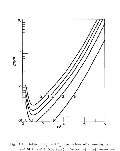
Figures 75

References 78

CHAPTER 4. STATISTICAL MECHANICS AND LIFSHITZ THEORY: II ARBITRARY SURFACE POTENTIALS

4.1. Introduction 81

4.2. Formalism 82

4.3. Asymptotics: Weak Interaction 84

4.3.1. Preliminary remarks 84

4.3.2. Asymptotic equations 85

4.4. Conclusion 88

References 90

CHAPTER 5. INTERACTION OF TWO SPHERES IN ELECTROLYTE

5.1. Introduction 91

5.2. Solution in Spherical Polar Coordinates 93

5.3. Series Solution of the Helmholtz Equation in Bispherical

Coordinates 98

5.4. Conclusion 105

Figure 107

References 108

CHAPTER 6. DISPERSION FORCES BETWEEN BODIES OF ARBITRARY SHAPE

6.1. Introduction 109

6.2. Basic Formalism 111

6.2.1. Formulation of the problem 111

6.2.2. Derivation of the Green function 113

6.3. The Single Surface 120

6.3.1. Preliminary remarks 120

6.3.2. Flat plate approximation 121

6.3.3. Corrections due to curvature 123

6.4. Two Interacting Bodies 129

6.4.1. Preliminaries 129

xi

6.4.3. Curvature corrections 131

6.4.4. Specific geometries: spheres, cylinders and

paraboloids 134

(a) Spheres 134

(b) Cylinders 135

(c) Elliptical paraboloids 136

6.4.5. Comparison with results for dielectrics 137

6.5. Conclusion 139

CHAPTER 1

CHAPTER I : Introduction

The calculation of van der Waal’s or dispersion forces is of importance in many fields. These range from the classical case of van der Waal's gases, where it was first realized that some sort of

attraction between neutral molecules must exist, to applications in the

1 2

fields of fibrous bed filters , biological cell-cell interactions , 3

liquid crystals , mineral flotation and colloid and polymer science in 4-6

general , to name but a few. A detailed account of the scope of applications of these forces would take many pages, and is beyond the

7 8

compass of this thesis, so this task is left to others * , except where it impinges directly on the subject matter. In order to set this work in its context however, a brief quasi-historical survey of the develop­ ment of the theory of van der Waal's forces is presented, dwelling on those contributions which are particularly relevant. Consequently, what follows is necessarily incomplete and lacking in balance.

London's calculation of the force between molecules, on the basis of quantum mechanics, may be seen as the fore-runner of the modern

g

2

shown to break down significantly when one is considering interactions between condensed media. This is because the force that a molecule

(represented as a fluctuating dipole) in a particle experiences due to a dipole in a second particle, is "screened" by the other dipoles in the two particles, so that the molecules do not simply interact in a pairwise manner.

9

In 1956 Lifshitz developed a macroscopic approach to the problem of van der Waal’s forces between condensed media. In this approach the effect of screening is taken into account by using the macroscopic dielectric constant, together with the macroscopic form of Maxwell's equations. Lifshitz calculated the force of attraction between two dielectric half spaces separated by a vacuum by means of the Maxwell stress tensor. His work has provided the basis and the impetus for subsequent research into dispersion forces, of which this thesis forms a part, and has made possible the comparison of theoretical predictions with experimental data^0 ^ . Numerous extensions and simplifications of

Lifshitz's original results have been reported. These include extensions taking into account the effect of an intervening medium"^, and interactions between bodies of certain fairly simple geometric shapes^ Attempts have also been made to include the effect of spatial dispersion in the interacting media; in particular, electrolytes have been the subject of much research because of their fundamental importance in many practical situations“^.

One major simplification was due to van Kämpen, Nijboer and 21

Schram , who showed that the Lifshitz result could be obtained by summing the change in the zero point energy of the normal surface modes of the system. Their approach has been extended to cover the case of

22 23 24

retardation * and finite (non zero) temperatures , as well as to 17-19

3

Langbein has developed a microscopic approach in the spirit of London and Hamaker, based on the Drude harmonic oscillator model of matter. By explicitly taking screening into account he was able to rederive van Kämpen et^al_'s result on the basis of this model, thereby gaining some understanding of the range of validity and the limitations

23 26 7

of the theory of van Kämpen et_ al_. Davies * and Langbein have shown the equivalence of these approaches to that used by Lifshitz, involving

27 the Maxwell stress tensor, and to another method Langbein has developed , involving the use of the Schröedinger equation. The connection between the macroscopic and microscopic theories is made via the law of Clausius- Mosotti, relating the dielectric constant to the molecular polarizabilities.

The basic approach underlying all these methods, which we may call the normal mode approach, is this. In order to obtain the free energy of interaction between macroscopic particles, we first of all

obtain a secular determinant for the system from the solutions of Maxwell's equations, whose zeros are the normal modes of the system. The logarithmic derivative of the secular determinant has simple poles at the normal mode frequencies co_., which we sum with weighting factor £n[ 2sinh (hco V2kT) ] , the free energy of an oscillator of frequency ok . This is the basis of the theory presented in ref. 8.

7

In a recently published book , Langbein extends this approach by introducing the second-quantized Hamiltonian, which accounts exactly

4

susceptibility, in place of the susceptibilities obtained from molecular polarizabilities. This susceptibility formally accounts for such effects as spatial dispersion and inhomogeneities.

Langbein's rigorous and somewhat formal approach lends itself to generalizations and extensions with comparative ease, in contrast to some of the alternative approaches. Furthermore, it often results in a clearer and more unified picture of the physical processes involved. One example of this is the facility with which he is able to deal with different geometries, and extend these results to include retardation

(see for example the relevant parts of ref.7). However, as a by-product of this all-encompassing approach, many of the expressions which result from his work are very complicated and difficult to evaluate, and

simplifications are not always obvious. Also, as these expressions are in the form of perturbation expansions, they are subject to all the usual restrictions of the latter.

5

Alternatively, in some cases we can begin with a macroscopic Hamiltonian, so that we are dealing with macroscopic quantities at all times (cf. the

28 29

work of Buff and Stillinger , and Gorelkin and Smilga on electrolytes). Another practical requirement of any realistic theory is that the resulting

formulae must not be so involved as to make computation impossible. In order to satisfy these requirements, we are generally restricted to applying normal mode theory in practical situations. However, in places where

the limitations of normal mode theory are apparent, we may expect that applications of this more general theory of Langbein will lead to significant improvements over the existing theory.

30

In a recent note , Davies has shown that the theory of Lifshitz is in fact a perturbation approach, as we have already implied. By

31

comparing this approach to one originated by Craig , and since simplified 32

and extended by Mitchell and Richmond , he has shown that Craig's results only reduce to Lifshitz's if the polarization operator is assumed linear in the coupling constant. For the interaction between dielectric particles this is a good, assumption equivalent to the R.P.A. approximation, and

no difficulties arise. However, for non-uniform situations such as the interaction between charged particles in electrolyte solution, the assumption is simply not true, and qualitatively different results may be obtained by the two methods as we show in Chapter 3. In order to discuss the different theoretical approaches of Craig and Langbein, we briefly outline the former here.

31

6

33

way . Part of this expectation value is identified with a macroscopic Green function for the response of the system, which he then calculates via Maxwell’s equations; the identification follows when the expectation value of the quantum mechanical number density operator multiplied by the electronic charge is equated with the macroscopic charge density.

This process replaces the use of the law of Clausius-Mos otti in Langbein’s formalism, in relating microscopic to macroscopic quantities. The end result is a sum over frequencies on the imaginary axis, which is the case for Langbein also. By using the method of the coupling constant

integration, he formally avoids the perturbation expansion of Langbein. Of course, the two approaches must rigorously yield the same answer for the thermodynamic potential (the free energy); the difference comes in the way in which approximations enter into the two theories, in the evaluation of the susceptibilities and the Green function.

At this stage perhaps we should remark on the formalism which we have attributed to Craig. In actual fact, the essentials of this formalism are well known, and can be obtained from ref. 33. Furthermore, the way in which Craig derives his Green function for spatially dispersive media is questionable, though his results should hold for non-spatially dispersive media, and are certainly capable of extension to include spatial dispersion, as we indicate in the next cahpter. Nevertheless, we choose to designate this approach as Craig's formalism, as he appears

to have been the first to apply it to the case of dispersion forces. 34

Very recently, Agarwal has published a series of papers in which he

7

We now turn our attention to the interactions of particles in dilute electrolyte solution. It turns out that for the case of non-uniform electrolyte (where surface charges are present) Craig's formalism

35

provides a very useful method of approximation . The electrolyte is modelled as an interacting electron gas in an external field, except that the particles, being macroscopic, are assumed to obey Boltzmann statistics in the calculation of the macroscopic charge response Green function, calculated on the basis of Maxwell's equations. This approach is of course valid only for static terms,» due to the use of the Boltzmann factor. However for temperatures of interest (i.e. near room temperature) it can easily be seen that the electrolyte has a significant effect

35

on these terms only ; the remaining part can be calculated ignoring the spatial dispersion due to the ions in the electrolyte in the usual way for dielectrics.

Langbein's formalism apparently does not lend itself quite so easily to computation of dispersion forces in electrolyte, and this has not been attempted so far (beyond normal mode theory, that is). It should be rewarding to apply Langbein's theory in order to throw light on certain difficulties which arise in the application of Craig's formalism to

the theory of electrolytes, concerning the dependence of the adsorption 35

potential on the coupling constant

There is one final point of comparison. In Lifshitz's original 9

work , as in most of the later research, it is found that the sum over frequency may be written as a sum over positive frequencies only (i.e. frequencies with a positive imaginary part) and this result is also

30

obtained by Mitchell and Richmond from Craig's formalism. However, Langbein finds that the frequency sum should extend over positive and

7

8

Mitchell and Richmond obtain their result by an alternative approach remains a question. The answer seems to lie in their assumption that the expectation value of the response temperature Green function is

purely real on the imaginary frequency axis. Rather they should introduce 36

retarded and advanced temperature Green functions , in an analogous 37

9

REFERENCES

1. K.W. Sarkies and J.W. Perram, A.J. Ch. E. Journal, 1972, 18, 1255-1257.

2. V.A. Parsegian, Ann. Rev. Biophys. Bioeng., 1973, 2_, 221-255, and references cited there.

3. E.R. Smith and B.W. Ninham, Physica, 1973, 66, 111-130.

4. C.J. Barnes and B. Davies, J. Chem. Soc. Faraday II (to appear). 5. D. Chan, D.J. Mitchell, B.W. Ninham and L.R. White, J. Chem. Soc.,

Faraday II (to appear).

6. The above references are intended as examples of literature in their respective fields. A more comprehensive listing of some parts of the literature may be found in refs. 7 and 8 below. 7. D. Langbein, ’’Van der Waal's Attraction", Springer Tracts in Modern

Physics, Springer, Berlin, 1974.

8. J. Mahanty and B.W. Ninham, "Dispersion Forces", Academic Press, 1975.

9. E.M. Lifshitz, Sov. Phys. J.E.T.P., 1956, 2, 73-83.

10. P. Richmond, B.W. Ninham and R.H. Ottewill, J. Coll. Inter. Sei., 1973, 45_, 69-80.

11. P. Richmond and B.W. Ninham, Solid St. Comm., 1971, 9^, 1045-1047. - - J. Low Temp. Phys.- 1971, 5, 177-189.

12. E.S. Sabisky and C.H. Anderson, Phys. Rev., 1973, A7_, 790-806. 13. P. Richmond and B.W. Ninham, J. Coll. Inter. Sei., 1972, 4 0 , 406. 14. J.N. Israelachvilli and D. Tabor, Nature Phys. Sei., 1972, 236, 106. 15. I.E. Dzyaloshinskii, E.M. Lifshitz and L.P. Pitaevskii, Adv. Phys.,

1961, 10, 165-209.

16. D. Langbein, J. Adhesion, 1969, 1, 237-245. - - Phys. Rev., 1970, B2_, 3371-3383.

- - J. Adhesion, 1972, _3, 213-235

10

17. D.J. Mitchell and B.W. Ninham, J. Chem. Phys., 1972, 56, 1117-1126. - - J. Chem. Phys., 1973, 59, 1246-1252.

18. D.J. Mitchell, B.W. Ninham and P. Richmond, J. Theor. Biol, 1972, 37_, 251-259.

- - Biophys. J., 1973, 13, 359-369. - - Biophys. J., 1973, 13, 370-384.

19. B.W. Ninham and V.A. Parsegian, J. Chem. Phys., 1970, 52, 4578-4587. - - J. Chem. Phys., 1970, 53, 3398-3402.

20. B. Davies and B.W. Ninham, J. Chem. Phys., 1972, 56_, 5797-5801. See also other references cited in Chapter 3 of this thesis. 21. N.G. Van Kämpen, B.R.A. Nijboer and K. Schram, Phys. Lett, 1968,

26A, 307-308.

22. E. Gerlach, Phys. Rev., 1971, B4, 393-396. 23. B. Davies, Phys. Lett., 1971, 37A, 391-392.

24. B.W. Ninham, V.A. Parsegian and G.H. Weiss, J. Stat. Phys., 1970,

2j 323-328.

25. D. Langbein, J. Phys. Chem. Solids, 1971, 32, 133-138. 26. B. Davies, Chem. Phys. Letters, 1971, 16^, 388.

27. D. Langbein, J. Phys. A, 1971, £, 471-476.

28. F.P. Buff and F.H. Stillinger, J. Chem. Phys., 1963, 39, 1911-1923. F.H. Stillinger and F.P. Buff, J. Chem. Phys., 1962, 37, 1-12.

29. V.N. Gorelkin and V.P. Smilga, Zh. Eksp. Teor. Fiz,m 1972, 63_, 1436-1443. V.P. Smilga and V.N. Gorelkin, Research in Surface Forces, 1971,

3, 151-163.

30. B. Davies, Phys. Letters, 1974, 4 8 A , 298-299. 31. R.A. Craig, Phys. Rev., 1972, B6, 1134-1142,

- - J. Chem. Phys., 1973, 58, 2988-2993.

32. D.J. Mitchell and P. Richmond, J. Coll. Inter. Sei., 1974, 46, 118-127. - - J. Coll. Inter. Sei., 1974, 46, 128-131.

11

33. See for example L.P. Kadanoff and G. Baym, "Quantum Statistical Mechanics” , (Benjamin, N.Y., 1962).

34. G.S. Agarwal, Phys. Rev. A, 1975, n , 230-242. - - Phys. Rev. A, 1975, 11_, 243-252.

- - Phys. Rev. A, 1975, 11, 253-264. 35. See Chapter 3 of this thesis.

CHAPTER 2

12

CHAPTER 2: Spatial Dispersion

2.1. INTRODUCTION

In order to obtain the dispersion or van der Waal's interaction between a system of particles, most of the methods discussed in Chapter 1 require the solution of Maxwell's equations for the system, or can be reduced to an expression involving those solutions. In their most general macroscopic form, Maxwell's equations may be written"^

V . D = 4ttp

V x E

v • B

1 3

?

(2.1)

v x H 4tt 1

c ~ + c 9t

where p and J are the free charge and current densities respectively. This system of equations is generally closed by assuming a relationship between D and E, and between B and H. For simplicity, we assume that the media

with which we are concerned are non-magnetic, so that B = H. If the electric displacement D is linearly related to the electric field E (which it is if the fields are sufficiently weak) it is customary to define a dielectric tensor £, so that

D(r) = £(r) E(r) . (2.2)

However this equation implies that the relationship between D and E is not only linear, but also local. The most general linear relationship between D and E2,3 is

D(r) = / d 3r e(r,r') E(r') (2.3)

13

relationship is in general very difficult to handle, and so the need arises to obtain approximations for the kernel £(r,rf) of the integral in Eq. (2.3). We have supressed the role of the time variable in Eq. (2.2) and (2.3), as we can always assume that the various quantities have time dependence given by a factor exp(-iwt), as long as the material properties do not change with time^^.

For problems concerning dispersion forces between macroscopic particles, we are generally concerned with relatively long wavelength electromagnetic waves, which do not vary appreciably over distances the size of microscopic inhomogeneities, and so we can neglect these variations in the field at the molecular level. (This procedure is not without

difficulties however, and leads to divergences in surface energy calculations5 , and in the energy of adsorption of a molecule on a surface. It is possible to overcome these difficulties by fairly intuitive arguments, either by

/ T O

assuming a finite "size,: for a molecule , or by assuming a continuously varying dielectric constant across the boundary5,9. Both of these

alternatives are useful ways of allowing for spatial dispersion at the molecular level, but it appears that the former one is the more straight­ forward approach.)

14

case of spatial dispersion in crystals, which would seem to be ruled out by the above assumption of homogeneity, can nevertheless be treated in the same manner, and the reader is referred to the detailed discussion of section 4.1 of ref. 3 for justification.

In the bulk or interior of substances exhibiting spatial dispersion (that is, far from the surface) the dielectric constant is a function of

|r-r'I only, in our approximation, and the integral in Eq. (2.3) becomes a convolution. Then we are able to define a wave-number dependent dielectric constant, e_(k,w), as the Fourier transform (in four dimensions) of

e(r,r’; t,t') = e(r-r’; t-t')3 . The presence of a boundary alters this situation rather, and for simplicity we consider a planar boundary between a semi-infinite spatially dispersive medium, and a vacuum. We shall also assume that the bulk of the spatially dispersive medium is isotropic as well as homogeneous throughout. Then the response at r to an impulse at r T can depend only on the distances |r-r* | and |r-r' |, where r* is the mirror image of r' in the plane defined by the interface. This is a

consequence of the physical requirement that an impulse at r' propagates to r either directly, or by way of reflection at the surface.

Since our system is inhomogeneous in the z-direction only, the surface being the plane z=0, we can take Fourier components in the x and y directions, and write in place of Eq. (2.3)

D(r) — — / d 2q / dz' e^9‘^ e(q; z-z', z+z')E(q,z')dz' (2.4) (2tt)

where q = (k^,k^,0) and the symbol ~ denotes the (two-dimensional) Fourier transform.

15

£ (q,z-z',z+z') = e 0 (q,z-z’) + £(q,z+z') (2.5)

/\ ^

where e 0 (q,z-z') is the bulk dielectric constant, and £^(q,z+z') accounts for the presence of the surface. It is not clear though, precisely what form the function e 1(q,z+z') should take.

Even for bulk spatially dispersive media in the free electron-gas approximation, the exact form of the dielectric constant is extremely

12

complicated , and obviously some sort of approximation is needed in order to obtain a form useful for calculation of dispersion forces. The need for such an approximation gives rise to the use of additional boundary

conditions (a.b.c's) for Maxwell's equations, and there has been considerable 2 3 11 13-19 discussion in the literature as to the eaxct nature of these * * *

Clearly, if the exact constitutive relationship between D and E is known, no further approximation is necessary, and Maxwell's equations formally yield complete solutions when taken with the usual Maxwell boundary

conditions. The a.b.c.'s arise out of the need to be able to calculate the Green function of the system (say) in a simple form, given the Green functions for the bulk constituent media.

Two particular a.b.c. 's representing virtually opposite limits have been commonly used, although some more general a.b.c.'s have also

3 11 19

been proposed * ’ . All of these boundary conditions overcome the lack of knowledge of the dielectric constant near the boundary by using the bulk dielectric constant in one form or another.

13 14

The first of these a.b.c.'s 5 , obtained by letting

e1(q,z+z') = e 0(q,z+z'), can be shown to be equivalent to assuming specular reflection of the charged particles (usually electrons) at the boundary.

10

Davies and Ninham obtained this boundary condition for electrolytes on the basis of a hydrodynamic model of ion transport; the same result can also be obtained on truncation of the Boltzmann-Vlasov system at the third

16

14-17

The remaining boundary condition assumes that the bulk

dielectric constant holds good right up to the boundary, so that e1 (r,r')=0. In the same terms as we described the first a.b.c., this one may be seen

14 to correspond to diffuse reflection of the charge carriers at the boundary

We choose to investigate these a.b.c.'s because the Green function for the system is particularly simple in these two cases. Also, since they do in a sense represent two opposite limiting cases, we might hope to use one or the other as an approximation to the real state of affairs by consideration of the physical situation. Specular reflection, because of

21

its similarity with the bulk response , leads generally to simpler results than diffuse reflection, (see ref. 14 for example) and for this reason has until recently been more widely used. However, this boundary

14 19 condition leads to results which are at variance with experiment ’ , and this has led to consideration of other a.b.c.'s. Consequently, and for reasons mentioned before, we feel justified in considering the diffuse reflection a.b.c., despite the criticism that has been brought to bear

•. 18 upon it

2.2. EXPLICIT FORM OF THE a.b.c's

For semi-infinite media, the assumption of specular reflection leads to particularly simple solutions of Maxwell's equations and dispersion relations, as Flores shows in ref. 21. In the non-retarded case, the

van der Waal's interaction between half-spaces of dispersive media across a dielectric slab, or the opposite case of a film of spatially dispersive medium, may be handled by an analogous method to that used by Davies and Ninham^, at least for the longitudinal wave-number dependent dielectric constant of the form (we use the notation of ref. 15)

e(k,co) = e0(w) + x(^) / (k2 - y 2 (oo)} (2.6)

17

that the effects of spatial dispersion on the van der Waal’s interaction

-h

between macroscopic bodies will be unimportant unless the quantities X or y, which have the dimensions of length, are of the same order of

magnitude as the separation. (See for example Langbein's work on adsorbed layers in ref. 5, where it is found that the effect of adsorbed layers is minimal unless their thickness is comparable to the separation.) This means that for crystals certainly, and probably for metals also, spatial dispersion is not expected to play a significant role when the interaction is retarded. Since the non-retarded case is covered implicitly by the work of Davies and Ninham, we feel justified in restricting ourselves to the diffuse reflection boundary condition for the sake of simplicity. The more general case where retardation is included is a simple extension of this work, and we could give a counterpart to each equation of the subsequent analysis covering this case also.

We consider a film of spatially dispersive medium, since the restriction to semi-infinite half spaces introduces simplifications to the a.b.c.'s which are non trivial. Furthermore, experimental evidence for

22

spatial dispersion in thin metallic films has long been known . The slab of spatially dispersive material is bounded by the planes z = ±d. Then we find that D and E are related by the constitutive equation

D(r) =

9 ., exp[ i (k -k') z]

---

- f

e

-k')d]---(2tt) 4 ~ z ~ ~ ~ z z U z

V

(2.7)

where we assume S(k) is a scalar (i.e. L .

00

cQOqp

k'

z ± w_J. Im w. ^ 0 .

Provided that e(k) has only simple poles on the real axis, we can split

18

t h e i n t e g r a l o v e r i n t o two p a r t s , and e v a l u a t e e ac h p a r t as a sum o v e r

t h e r e s i d u e s a t t h e p o l e s o f £ ( k ) , c o m p l e t i n g t h e c o n t o u r o f i n t e g r a t i o n

as a s e m i - c i r c l e o f i n f i n i t e r a d i u s i n t h e u p p e r h a l f p l a n e i n t h e one

c a s e , and t h e l o we r h a l f p l a n e i n t h e o t h e r . Then Eq. ( 2 . 6 ) c a n be

r e w r i t t e n

D ( r ) --- J d k e ~ ~1 r , 3l i k . r (2tt)

e (k ) + 2 3

exp[ i (w. -k ) (z+d) ] _______3 z______

(w. - k ) v j z J

exp[ i ( w . +k ) ( z - d ) ] ________3 z________

w. + k 3 z

Res e ( q , k ' ) , I ~ z k =w.

z 3

E(k)

( 2 . 9 )

S u b s t i t u t i n g Eq. ( 2 . 9 ) i n t o ( 2 . 1 ) we o b t a i n an e q u a t i o n f o r t h e e l e c t r i c

f i e l d E i n t h e a b s e n c e o f f r e e c h a r g e and c u r r e n t d e n s i t i e s :

—- — / d 3k e 1- ' -

J

(2tt) 3

(2.10)

+ 2

3

e x p [ i ( w . - k ) (z+d)] e x p [ - i ( w . + k ) ( z - d ) ] ' _______3 z________ , _________ 3 z

(w. - k )

3 z (w. + k ) 3 z

Res e ( k * ) E(k) k ' = w.

z 3

By r e q u i r i n g t h e c o e f f i c i e n t o f e^Wj Z and e ^Wj Z t o v a n i s h i n d e p e n d e n t l y

f o r e ac h j , we hav e

i _ / d 3k e i k - r e x p [ i ( w . - k z K z . d ) ]

(277) _{(W. - k )}

3 z

(277)

/ d 3kei k . r exP t i ( wj +k z ) ( z - d ) ] (w. + k )

3 z

Res e ( k ' ) E(k) k ' = w.

z 3

Res e ( k ' ) E(k) k ' = w.

z 3

(2.11)

Then t h e r e m a i n i n g t e r m s i n ( 2 . 1 0 ) p r o d u c e e x a c t l y t h e same

d i s p e r s i o n r e l a t i o n s as a r e o b t a i n e d i n t h e b u l k . T h i s r ema r k a p p l i e s

a l s o t o s p e c u l a r r e f l e c t i o n , and i s a c o n s e q u e n c e o f c h o o s i n g e ( r , r ’ ) t o

19

introduced. We define the longitudinal and transverse parts of E(k) as

k(k.E)/k2 and

-k x (k x E)/k2

respectively. The dispersion relations for k^ corresponding to longitudinal modes are

e(k) = 0 (2.12)

while the transverse modes are given by

k 2 - ^ e(k) = 0 . (2.13)

c The a.b.c.'s then take the form

2 (w.-o l) 1 exp[ i (w. -OL)d]

1 ^ 1 ^ 1

2 (w -o l)"1 exp[ i (w -OL)d]

i J ^

Res

k ' = w .

z 3

Res

k ' = w .

z 1

e(k?) 5Ck±D

e(k') E(k.)

0

0

(2.14)

where the index i runs over all the zeros ou of the dispersion relation (2.12) and C2.13); and k. E (k , k , a.). From the definition of the

»V i x y i

longitudinal and transverse parts of E, we find the Fourier components E(k^) to satisfy two further relations

k ± x [ki x E(ki)] = 0 (2.15)

where is a zero of (2.12), and

k ± . E(ki) = 0 (2.16)

where ou is now a zero of (2.13). In the absence of free charge the longitudinal part of D is clearly zero, and we can write

D(r) = / d 2q e1^ 2 e(ki) E ( k ^ e'°j2 (2.17) transverse

modes

20

(2.1) to be

fgw

transverse modes

k. x E(k.)el<Tiz (2.18)

Our results reduce to those of A g a r w a l , Pattanayak and W o l f ^

when the dielectric constant is of the form (2.6). They are easily

generalised to include the case of anisotropic media, such as when the

dielectric constant m u s t be written in terms of a longitudinal and a

10 12 3

transverse part * , or an anisotropic crystal . In the first case

E q s . (2.12) and (2.13) are replaced by

and

eL (k,w)

. 2 0J2 .

k ---o' e (k >w)

(2.19)

where e (k,w) and e (k,w) are the longitudinal and transverse dielectric

constants respectively.

In the non-retarded limit we can either take the limit

°VC 0

in Eq. (2.14), or work with the non-retarded form of Maxwell's equations

from the start. In this case only the longitudinal dispersion relation

(2.19) is required (plus the dispersion relation, k 2 = 0). Defining an

electric potential (f)(r) by the relationship E(k) = -ik (f>(k), the equations

corresponding to (2.14) and (2.17) are

q 2+a.w.

2 ---- Res e(k') <f>(k.) = 0

i (w. - a. ) k ' = w .

3 1

z

q -a.w.

2 ---- i-J- Res e(k') $(ki)

i (w.+a.) k'=w.

3

i

z

(2.21)

and

D(r) / d2q eiq.r _{e ( kq) t}

_{§tk+q)eXp("qz)}

+ 2 2

i j

exp[ i(w.-ol ) (z+d)] exp[ i(w.+cu) (z-d)]'

---

— 1--- + ---

—

1---(2.22)

O j - o l) ( w . + a . )

3

i

Res e(k') E(k.)

k '= w . ~ ~

21

The sum over i runs over the zeros ou of the longitudinal dispersion relation (2.12) or (2.19) only, and k+ is the vector (k , k , ±iq).

2.3. INTERACTION FREE ENERGY

Having determined the structure of the propagating modes in a bounded spatially dispersive medium, we are now in a position to calculate the interaction free energy of two dielectric half spaces across a

spatially dispersive slab, or vice versa. The a.b.c's (2.14)-(2.16), or (2.15) and (2.21), together with the usual Maxwell boundary conditions are just sufficient to exactly determine the non-zero coefficients E(k.) of the electric and magnetic fields in the medium, and so we are in a position to calculate the secular determinant or Green function of such a

system. The more general case of two spatially dispersive half spaces (dielectric constants ea (k,w), e (k,w) etc.) interacting across a third slab of dielectric constant e3 (k,w), which exhibits spatial dispersion, can also be treated by this method. However, in that case it is not at all clear that either of the two boundary conditions considered are

adequate. Nevertheless, because this general case includes the two first mentioned systems as limiting cases, and because very little extra effort

is required, we choose to consider this more general case. Further, we specialize now to spatially dispersive media whose dielectric constants are of the form (2.6) in order that our results may be simplified as much as possible. Since this form arises in the hydrodynamic treatment of a plasma, of which ref. 10 may be taken as an example; as well as in the effective mass approximation for c r y s t a l s t h e restriction to this form is not as limiting as may first be supposed. In any case, the more general form, as dealt with in the previous section, offers no further conceptual difficulties than this simple form provides.

22

8 23

C r a i g ’s formalism * . However, if we assume that x( w ) is linearly

dependent on the coupling constant, while JJ2 (oj) is coupling constant

25

independent, Davies has shown that the free energy m ay be obtained from

the logarithm of the secular determinant, and that is the approach we

shall adopt here, thus avoiding the coupling constant integration.

We have already noted the fact that for the dielectric constant

(2.6), our results from section (2.2) reduce to those of ref. 15, and

we quote their results relevant to our system. In terms of the

two-dimensional Fourier transform, the electric field, displacement and

magnetic field are given respectively by

E ( q , z ;w)

D ( q , z ;w)

B(q,z;w)

2 A . (q, 03) exp(ia.z)

j = l ~3 ~ 3

4

2

j=l

c w

e n (w)-l x O )

a .2-w2

1

A_. exp(icfjz)

2 B. exp(ia.z)

j=i ~J 3

C2.26)

where : j = 1,...,4 are the roots of

4 2

Ö ~ O roo2

lc

e - q 2+ w 2

2 o + W ‘

rco2 ;

— e o - *

lc

_ X — = 0 (2.27)

and a. : j = 5,6 are the roots of

1

Q - W2 + X_ (2.28)

Im g . < 0 i = 1,2,5 ;

a3

2

6

5

and w is given by

w 2 = y 2 - q 2 ; Re w > 0 , Im w > 0

In addition, the coefficients must obey the following constraints

(kj . A_.) k_. = 0 j = 1, ... , 4 (transverse modes)

23

exp[ -i (ct_. -w)dl j=l ~J

(a j -w)

6 y a

exp[ i (Oj +w)d]

=

j=l

(aj+W)

B. = k. x A. _{j = 1, • -},. , 4

k. (k , k , a.)

x* y

y

(2.29)

The remaining relationships needed to obtain the secular determinant are provided by the Maxwell boundary conditions, involving the continuity of E^, Ey and across the boundary at z = ±d. Making use of these, as well as the first two and last two relations in (2.29), leads to the equations

4

j =1

j=l iz 2 j j

where G_.^ are the relevant roots of (2.27) or (2.28) in medium i, ck = 6

s A. q 2a. j=5 jz 1

6

2 A. q " G .

j=5 JZ 3

: (2 .27) or

(2.30)

a i3 > X,

£ji = £ .01 +

a ..2 - w.2

Ji i

6. = e * + a. e .*

1 ll 1 21

y. = a . + a. a . - q2$./a .

'i n 1 21 H i 5 1

ai =

-a .+w. a .o .+q‘

21 1 n 51 n

a .+w. a .a .+q2

11 1 21 51 n

3;

a .+w. (a .-g .)a_.

51 1 ^ 1 1 2i'( 5 1

a.. +w

ii i G2i si

24

multiplicative factor o l"1 into Eq. (2.30), which we can ignore.

Equations (2.29) and [2.30) yield a system of linear homogeneous equations in the coefficients A. . If they are to be consistent, we obtain a

six-jz

by-six secular determinant, D E [oo,q), which is given explicitly in the appendix. The dispersion relation for the normal modes is then

DE (üi,q) = 0 . (2.31)

In a similar manner, we can obtain another homogeneous linear system of equations in the coefficients B_. ^ from Eq. (2.29) and the Maxwell boundary conditions involving the continuity of tangential components of H and the normal components of B across the boundary. Consistency requirements then lead to a further dispersion relation

DM (w,q) = 0 (2.32)

where D^(oo,q) is a four-by-four determinant, and is also given explicitly in the appendix. Using the methods of normal mode theory, as outlined in the first chapter, we may use (2.31) and (2.32) to obtain the dispersion free-energy of the system.

2.4. LIMITING CASES

In several limiting cases our results simplify, yielding known results in some cases. Firstly, if one assumes that the media 1 and 2 are spatially non-dispersive, then we can replace the factors y^ and 6^

occurring in the determinant DE (o),q) by and (=£q^) respectively. In the case = 1, our results give the dispersion free energy of a metallic film in vacuo. Conversely, if one assumes that medium 3 is

spatially non-dispersive, we find that we can write the secular determinant

as .

Dc (w,q) = A A e"2ia3d - 1 = 0

E n 1 2

T T - 20 d

= A1A 2 e 3 - 1 =

DM 0,q) 0

25

w h e r e A

6 i a 3 - e 3 q .

1

q a 3 + £ s y'i

Ä. i

V ? - a 3 V ' + ü 3

q 6. = e . (q2w.a .) -1 -1 VM 1 5 1 J

“ -W ia 5i+ (a ii+ a 2i)°5i X i

< V 0 li> (Wi'a 2i) 2 *

q y ± = a . a . a . +

11 21 51 (a . + a .v 11 21 - a .51^n ) q 2

v * '

' i = a . + a . + w.11 21 1

an d a

3 = a1 3

In the limit x^ 0, our results reduce to the usual Lifshitz 26

interaction between dielectric slabs

The limit oo2/c2 0 gives the non-retarded result, but we decline to quote the result here, as it is messy. It is suffice to say

10

that it only reduces to the result of Davies and Ninham in the limit

X- - 0 .

q2

Using Eqs. (2.33) it can be shown that in the case of two

spatially dispersive half spaces interacting across a dielectric, spatial dispersion contributes very little to the interaction free energy, except in the limit of small separation, when the distance x 2 becomes comparable

27

with the separation . This is in agreement with our hypothesis made at the beginning of Section (2.2). We note also, that the result appears in the symmetric form hypothesized by Agarwal in ref. 24, on the basis of

26

2.5. CONCLUSION

27

APPENDIX 2A

In this appendix we give the explicit form of the secular determinants D^(a3,q) and D^(u),q) of Section (2.3). The determinant Dg(w,q) is given by Eq. (2A.1), where the various symbols are defined

X i

X i in

in _to

to •H

•H X i i x i

CD in CD in

r—H _to 1—1 _{to x i}

1 •H 1 •H in

f-- \ CD x i r—\ 1 _to

£ rH in _£ CD

+_in i to i rH 1

/-- \ •H in I CD

ö <D to f-- N CM

'—y ₊ rH V—y

H in rH 1 pH

1 m to rH 1 m in l to

to v_y 1 m to to to

CM e r to CM v—y CM

e r •H CM e r e r e r

i i e r 1 •H i

X i X i

CM CM

to to

•H •H

X i CD X i X i i

X i CM t—N CM CM CD

CM _to r-H _{to to t-- \}

to •H > - •H •H CM

•H CD * i i >

-cd rH CO _{<D CD *}

r—1 _i rH rH CO

1 /-- \ 00 | i CM

/-- \ + /--\ r—'s 00

+ CO _{S £ 1}

+ <N CM 1 CO

CM to to CM CM CM

to v._y rH to to to

v—/ _{e r <o} v_y v—y CM

CM •H v—/ CM e r <o

to i i to •H v- '

X i_rH X i

rH

to to

•H •H

X i CD x i i

X i rH _{f-- N} rH _CD

rH _to rH _{x i to} f--\

to •H > - rH _•H CM

•H CD * to i >

-CD CO •H CD *

H 1 rH i pH co

i /-- \ OJ CD i rH

f-- \ iS + t-- \ f-- N 00

+ CO _{£ 1}

+ rH rH _{1 1}

CM _to to rH rH rH

to v_y cH to IO to

v—/ _{e r KO} v—y v_y CM

CM •H V__/ _{rH e r}

to i 1 to •H V—/

X3 in

to X!

•H in

i t o

CD X i •H

H in CD x i

i t o X! rH in

/---\ •H in l t o

I t o f---\ •H

i CD •H i S CD in

in rH i + rH t o

t o I CD in i •H

V---' _{f---\ rH t o f—\}

CD

rH 2 ‘O £ CM

1 m i rH rH +

t o in 1 m 1 m in pH

t o t o t o t o i in

CM V_J _{CM CM v_y}

t o

e r e r e r e r e r CM

i •H 1 i •H e r

x i x i

CM CM

t o t o

•H •H

X i X i i x i e D

CM CM CD X i CM /*~\

t o t o /---\ CM t o CM

•H •H rH t o •H >

-i i f — •H CD *

CD CD * CD rH CO

r l rH co rH | CM

1 i CM i f---\ 00

r—\ t—\ 00 /---\ 2£ +

£ i i S + co

i i CO ₊ CM CM

CM CM CM CM t o t o

t o t o t o t o v—y CM

V__/ V—y r l v—y _{e r} < o

CM e r CM •H v._y

to •H v—y _{to i i}

X i x i

rH rH

to to

•H •H

X) X J i x i CD

rH rH _{CD x i} rH /—\

to to t---\ rH _to CM

•H •H rH _{to •H >}

-i i > - •H CD *

CD CD * CD rH CO

rH r-H CO rH _i rH

| 1 rH _i f—\ 00

r—\ f---\ 00 /---\ +

1 i S + co

i i CO ₊ rH rH

rH rH rH rH _{to to}

to to to to v__y CM

V— y v_y rH ^_y _{e r}

r-H _{e r <o} rH •H v—y

1 ö •H v—y _{to i}

e r *N 3 ■p <D X i W

Q II

(2

A

.1

CM <

O l

29

T3

<M

t> •H 0

I

CM

t>

T3

CM

Ö •H 0

x s

CM

Ö •H I

0

I

+ CM

I

4-> 0 T3

II

/ —M O '

3

ll ll li

* * *

•H *H *H

> - ° o Ö

0

0 ,C

30

REFERENCES

1. W.T. Scott, "The Physics of Electricity and Magnetism", (Wiley, N.Y., 1959).

2. J.J. Hopfield, J. Phys. Soc. Japan, 1966, 2 1 , supplement. • 3. V.M. Agranovich and V.L. Ginzburg, "Spatial Dispersion in Crystal

Optics and the Theory of Excitons", (Interscience, N.Y., 1966). 4. D. Pines, "Elementary Excitations in Solids", (Benjamin, N. Y . , 1964). 5. D. Langbein, "Van der Waal's Attraction", (Springer Tracts in

Modern Physics, N.Y., 1974).

6. D.J. Mitchell and P. Richmond, Chem. Phys. Letters, 1973, 21, 113-114. 7. J. Mahanty and B.W. Ninham, "Dispersion Forces", (Academic Press,

London, 1975).

8. R.A. Craig, Phys. Rev., 1972, B6,1134-1142.

9. G.H. Weiss, J.E. Keiffer and V.A. Parsegian, J. Coll. Inter. Sei., 1973, 45_, 615-625.

10. B. Davies and B.W. Ninham, J. Chem. Phys., 1972, 5 6 , 5797-5801.

11. R. Zeyher, J.L. Birman and W. Brenig, Phys. Rev., 1972, B6^, 4613-4616. 12. M.G. Calkin and P.J. Nicholson, Rev. Modern Phys., 1967, 3 9 , 361-372. 13. R.H. Ritchie and A.L. Marusak, Surface Science, 1966, 4, 234-240. 14. J. Heinrichs, Solid St. Comm., 1973, 12, 167-170.

15. G.S. Agarwal, D.N. Pa ttanayak and E. Wolf, Phys. Rev. Letters, 1971, 27_, 1022-1025.

- - Optics Comm., 1971, 4_, 255-259. - - Physics Letters, 1972, 4 0 A , 229-280. 16. G.S. Agarwal, Optics Comm., 1972, 6_, 221-225.

17. A.A. Maradudin and D.L. Mills, Phys. Rev., 1973, B7, 2787-2810. 18. V.M. Agranovitch and V.I. Yudson, Optics Comm., 1973, 7, 121-124. 19. D.E. Beck and V. Celli, Phys. Rev. Letters, 197 , 28, 1124-1126.

31

21. F. Flores, II Nuovo Cimento, 1973, 14B, 1-14. 22. P. Schmüsser, Solid St. Comm., 1964, 2, 41- 43.

23. When this work was in final stages of preparation, a series of papers by G.S. Agarwal (see ref. 24) appeared, which synthesizes the theories of Craig's and others, and treats similar problems to those considered here, using the diffuse reflection a.b.c., and the same dielectric constant as Section 2.3.

24. G.S. Agarwal, Phys. Rev., 19 , All, 230-242 , 243-252 , 253-264. 25. B. Davies, Phys. Letters, 1974, 48A, 298-299.

CHAPTER 3

STATISTICAL MECHANICS AND LIFSHITZ THEORY FOR ELECTROLYTES

32

CHAPTER 3: Statistical Mechanics and Lifshitz Theory for Electrolytes: I: Small Surface Potentials

3.1. INTRODUCTION

The calculation of electrostatic and dispersion forces between bodies which are separated by an electrolyte is a problem of considerable importance in colloid science. It has been the general practice to

evaluate the electrostatic and dispersion contributions to the free energy 1_ 6

on the assumption that they may be treated independently, although

there is no firm basis for such a separation which is founded in the funda­ mental statistical mechanics of interacting systems. A common practice is

to define a phenomonological 'Hamaker constant* (usually independent of the salt concentration) so that those long range forces usually called *van der Waals* forces have a simple form, such as A/d3, where d is an interparticle separation. The electrostatic repulsion is then calculated from an argument which ignores dispersion forces, the treatment of Verwey and Overbeek^ still being in common use. Finally the two contributions are added.

Within the context of such a theory, various attempts have been made to give an expression for the Hamaker constant in terms of measurable quantities such as the dielectric data for the media and the Debye length

6 7

in the electrolyte. ’ Specific calculations involving electrolytes may

✓ 8-10

be found in the papers of Mitchell and Richmond and of Barouch, Perram

1112 6

and Smith * . The latter authors base their work on the Lifshitz theory , whereas the former authors commence from the fundamental equations of

statistical mechanics. Unfortunately, Mitchell and Richmond implicitly assume a certain linearity (in the coupling constant) which is in fact not

33

here that the Lifshitz approach is not completely invalid; rather it is based on an approximation which breaks down in a significant way for electrolyte systems, although it is still good for dielectrics separated by a macroscopic distance. We will return to a fuller discussion of these points later.

14-20

Several other formulations , aimed at obtaining the free energy of systems such as those we are considering, deserve comment. These

16 17 methods in general use expansion techniques, such as cluster expansions * ,

18 20

or Bogolyubov correlation functions * to determine the response of the electrolyte. The free energy is then obtained from semi-classical statis­ tical mechanics in a straightforward, self-consistent manner. The main difference between these formulations and the one presented here is that we approximate the ions as an interacting electron-gas in the presence of an external field. Then we are able to use the formalism of quantum statistical mechanics to write the final expression for the free-energy as the integral over the coupling constant of a Green function which

measures the response of the system, and which we identify with a particular macroscopic Green function. We are then free to calculate this Green

function macroscopically according to classical statistics, using whichever approximations are convenient. The method is somewhat similar to the use of experimental data for the dielectric constant in Lifshitz theory, which

13 is essentially restricted to the R.P.A. approximation

34

theory; for the purpose of the present work we use the simplest model available to obtain some interesting and new results. These results are presented in the next three sections. Section 3.3 is concerned with the single charged surface, while section 3.4 provides the necessary material to deal with overlapping double layers. The final section, section 3.5, presents numerical results for the overlapping double layers, and their significance in the light of some experimental work is discussed. In order to make this work more accessible to workers in the experimental aspects of colloid science we have relegated the necessary mathematics to five appendices. Appendix 3A deals with a general method for flat

plates, Appendix 3B with the mathematics associated with the single surface, while the last two appendices, 3C and 3D, deal with the mathematical formu­

lation of the overlapping double layers, and an asymptotic form of this formulation, respectively. Appendix 3E deals with refs. 15 and 40.

Many of our results are not new, but we believe that this is in itself a most useful part of the present work, because features which

15 1 previously seemed rather disconnected, sometimes in a quite puzzling way * are now shown to be part of a larger, consistent picture. Finally, we show that the theory predicts a repulsive force between overlapping double layers which is larger than that predicted by the conventional electro­ statics^. All of these features are discussed at length below.

3.2. BASIC FORMALISM 3.2.1 Craig’s formalism

35

2122

mechanics, and we follow the work of Craig * closely in what follows. To commence, we write down the Hamiltonian, viz.

H = 2 / ^ ( r ) H 0i|j (r)d3r + 2 / i|^(r)Ay (r)i^ (r)d3r

where ij^(r) is the particle annihilation operator for ions of type (charge, mass, etc.) a at position r, V is the Coulomb interaction potential, and

Ay^(r) is the energy of surface adsorption of the ions. The first term is the non-interacting Hamiltonian; that is, that part of the total

Hamiltonian which excludes the surface adsorption potential and the inter­ ion Coulomb potential. The other two terms are the ones which we wish to account for explicitly. Note that we have assumed that adsorption is an independent particle process except for the Coulomb interactions.

23 24

It is shown in many places * that the grand partition function Z = Tr[ e" ^ H-yN)] , 3 = 1/kT , (3.2)

where y is the chemical potential and N the total number of particles in 24 the system, and the free energy (actually the thermodynamic potential ) are given by

ft(= Q 0 + AQ) = -kTlnZ

- ß o + {1r - Fint<x> • (3-3) where

Fint(X) < AH1 (3.4)

and h' is defined by splitting the Hamiltonian in the form (we used an abbreviated, but obvious, notation)

H = Hq + H' . (3.5)