particulate materials
.
White Rose Research Online URL for this paper:
http://eprints.whiterose.ac.uk/147113/
Version: Submitted Version
Article:
Gower, A.L. orcid.org/0000-0002-3229-5451, Abrahams, I.D. and Parnell, W.J. (Submitted:
2019) A proof that multiple waves propagate in ensemble-averaged particulate materials.
arXiv. (Submitted)
© 2019 The Author(s). For reuse permissions, please contact the Author(s).
[email protected] https://eprints.whiterose.ac.uk/
Reuse
Items deposited in White Rose Research Online are protected by copyright, with all rights reserved unless indicated otherwise. They may be downloaded and/or printed for private study, or other acts as permitted by national copyright laws. The publisher or other rights holders may allow further reproduction and re-use of the full text version. This is indicated by the licence information on the White Rose Research Online record for the item.
Takedown
If you consider content in White Rose Research Online to be in breach of UK law, please notify us by
ENSEMBLE-AVERAGED PARTICULATE MATERIALS
ARTUR L. GOWER†, I. DAVID ABRAHAMS‡, AND WILLIAM J. PARNELL† §
Abstract. Effective medium theory describes an inhomogeneous material with macroscopic pa-rameters. To characterise wave propagation through an inhomogeneous material, the most crucial parameter is theeffective wavenumber. The most successful methods to calculate effective wavenum-bers developed over the last 70 years assume, with little justification, that the average wave in a random inhomogeneous material satisfies a wave equation, and therefore has a single effective wavenumber. By average, here, we mean an ensemble average over all possible inhomogeneities, which we consider to be particles or inclusions. Here we present a proof that theredoes not exist a unique effective (complex) wavenumber; instead, there are an infinite number of effective wavenum-bers. We also present the exact solution for the reflection coefficient when waves are incident on an inhomogeneous half-space. Results are presented for scalar waves and a two-dimensional material filled with randomly distributed particles. We also make use of standard statistical assumptions. Though there are many effective wavenumbers, we show through numerical examples that, in most parameter regimes, only a small number of these wavenumbers make a significant contribution to the wave field. The proof is based on the application of the Wiener-Hopf technique and makes no assumption on the wavelength, particle size/type, or volume fraction.
Key words. wave propagation, random media, composite materials, backscattering, multiple scattering, ensemble averaging, Wiener-Hopf
AMS subject classifications. 74J20, 45B05, 82D30, 78A48, 74A40
1. Introduction. Materials comprising particles or inclusions that are randomly distributed inside a uniform host medium occur frequently in the world around us. They occur as synthetically fabricated media and also in nature. Common examples include composites, emulsions, suspensions, complex gases, and polymers. Under-standing how electromagnetic, elastic, or acoustic waves propagate through these materials is necessary in order to characterise the properties of these materials, and also to design new materials that can control wave propagation.
The wave scattered from a particulate material will be influenced by the positions and properties of all particles, which are usually unknown. However, this scattered field, averaged over space or over time, depends only on the average particle properties. Many measurement systems perform averaging over space, if the receivers or incident wavelength are large enough [42], or over time [35]. In most cases, this averaging process is the same as averaging over all possible particle configurations. Such systems are sometimes called ergodic [35, 34]. In this paper, we focus on ensemble averaged waves, satisfying the scalar wave equation in two-dimensions, reflecting from, and propagating in, a half-space particulate material. In certain scenarios, such as light scattering, it is easier to measure the average intensity of the wave. However, even in these cases, the ensemble-averaged field is often needed as a first step [47,46].
One driving principle, often used in the literature, is that the ensemble-averaged wave itself satisfies a wave equation with a single effective wavenumber [11, 25, 10].
∗Submitted to the editors May 20, 2019.
Funding: This work was funded by EPSRC (EP/M026205/1,EP/L018039/1) including via the Isaac Newton Institute (EP/K032208/1,EP/R014604/1).
†Department of Mechanical Engineering, The University of Sheffield, UK ([email protected], http://arturgower.github.io).
‡ Isaac Newton Institute for Mathematical Sciences, 20 Clarkson Road, Cambridge CB3 0EH,
UK
§School of Mathematics, University of Manchester, Oxford Road, Manchester M13 9PL, UK
1
Reducing a inhomogeneous material, with many unknowns, down to one effective wavenumber is attractive as it greatly reduces the complexity of the problem. For this reason many papers have attempted to deduce this unique effective wavenumber from first principles in electromagnetism [48,45,34], acoustics [26,27,29,38,19] and elasticity [8, 39]. See [18] for a short overview of the history of this topic, including typical statistical assumptions employed within the methods, such as hole-correction and the quasi-crystalline approximation, which we also adopt here.
The assumption that the ensemble averaged wave field satisfies a wave equation, with an effective wavenumber, has never been fully justified. Here we prove that there
does not exist a unique effective wavenumber but instead there are an infinite number of them. Gower et al. [18] first showed that there exist many effective wavenumbers, and provided a technique, theMatching Method, to efficiently calculate the effective wave field. In the present paper and [18], we show that for some parameter regimes, at least two effective wavenumbers are needed to obtain accurate results, when compared with numerical simulations. We also provide examples of how a single effective wave approximation leads to inaccurate results for both transmission and reflection for a halfspace filled with particles, seeFigure 1.
Although the Matching Method developed in [18] gave accurate results, when compared to numerical methods and known asymptotic limits, the limitations of the method were not immediately clear. Here however we illustrate that the Matching Method is robust, because combining many effective wavenumbers is not just a good approximation, it is an analytical solution to the integral equation governing the en-semble averaged wave field. We prove this by employing the Wiener-Hopf technique and then, for clarity, illustrate the solution for particles that scatterer only in their monopole mode. The Wiener-Hopf technique also gives a simple and elegant expres-sion for the reflection coefficient.
The Wiener-Hopf technique is a powerful tool to solve a diverse range of wave scattering problems, see [9, Chapter 5. Wiener-Hopf Technique] and [24, 36] for an introduction. It is especially useful for semi-infinite domains [30, 37, 21, 49, 20, 6] and boundary value problems of mixed type. In this work, the Wiener-Hopf tech-nique clearly reveals the form of the analytic solution, but to compute the solution would require an analytic factorisation of a matrix-function. To explicitly perform this factorisation is difficult [3, 2, 5, 43]. Indeed this is often the hardest aspect of employing the Wiener-Hopf technique, although there exist approximate methods for this purpose [3, 22,4,1]. We do not focus in this article on these analytic factorisa-tions, as there already exists a method to compute the required solution [18]. Instead, the present work acts as proof that the Matching Method [18] faithfully reproduces the form of the analytic solution.
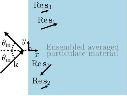
Figure 1 shows the main setup and result of this paper: an incident plane wave excites the half-spacex >0 filled with ensemble-averaged particles (the blue region), which generates a reflected wave and many effective transmitted waves. Thesp are
the transmitted wavevectors, and the smaller the length of the vector, the faster that effective wave attenuates as it propagates further into the material.
Ensembled averaged
particulate material
Re
s
2Re
s
0Re
s
1Re
s
3k
θ
inθ
iny
x
Fig. 1. When an incident plane wave eik·(x,y), with k = k(cosθ,sinθ), encounters an
(ensemble-averaged) particulate material, it excites many transmitted plane waves and one re-flected plane wave. The transmitted waves are of the form eisp·(x,y) with wavenumbers sp =
Sp(cosθp,sinθp)where bothSpandθpare complex numbers. The larger Imsp, the more quickly the
wave attenuates as it propagates into the half-space and the smaller the drawn vector for that wave above. The results shown here represent the effective wavenumbers for parameters(5.2), which are shown inFigure 3.
The dispersion relation (3.30), derived inSection 3, admits an infinite number of solutions, the effective wavenumbers. In Section 5, we deduce asymptotic forms for the effective wavenumbers in both a low and high frequency limit. In Section 6we compare numerical results for monopole scatterers, using the Wiener-Hopf technique, with classical methods that assume only one effective wavenumber [26, 29], and the Matching Method introduced in [18]. In general, when comparing predicted reflection coefficients, the Wiener-Hopf and Matching Method agree well, whereas the classical single-effective-wavenumber method can disagree by anywhere up to 20%. These results are discussed inSection 7together with anticipated future steps.
2. Waves in ensemble averaged particles. Consider a region filled with par-ticles or inclusions that are uniformly distributed. The field u is governed by the scalar wave equations:
∇2u+k2u= 0, (in the background material), (2.1)
∇2u+k2ou= 0, (inside a particle),
(2.2)
where k and ko are the real wavenumbers of the background and inclusion
materi-als, respectively. We assume all particles are identical, except for their position and orientation, for simplicity. For a distribution of particles, or multi-species, see [19].
Our goal is to calculate the ensemble average field hu(x, y)i, that is, the field averaged over all possible particle positions and orientations. For clarity, and ease of exposition, we consider that the particles are equally likely to be located anywhere except that they cannot overlap (this is often called thehole correction assumption). We also assume the quasi-crystalline approximation; for details on this, and for further details on deducing the results in this section, see [26, 19, 18].
[image:4.612.145.361.102.266.2]waves scattered by each particle, thejth scattered wave beinguj(x, y), we can write:
(2.3) u(x, y) =uinc(x, y) +
X
j
uj(x, y).
A simply and useful scenario to consider is when all particles are placed only within the half-space1 x > 0, which are then excited by a plane wave, incident from a homogeneous region:
(2.4) uinc(x, y) = ei(αx+βy), with (α, β) = (kcosθinc, ksinθinc),
where we restrict the incident angle−π2 < θinc< π
2, as shown inFigure 1, and consider
a slightly dissipative medium with
(2.5) Rek >0 and Imk >0.
This dissipation will facilitate the use of the Wiener-Hopf technique, and after reaching the solution we can takekto be real.
To describe the particulate medium we employ the following notation:
b= the minimum distance between particle centres, (2.6)
n= number of particles per unit area, (2.7)
Tn = the coefficients of the particle’s T-matrix,
(2.8)
φ=πnb
2
4 = particle area fraction. (2.9)
Although the area fraction φ, normally called the volume fraction, is a combination of other parameters, it is useful because it is non-dimensional. If we let ao be the
maximum distance from the particle’s centre to its boundary, then we can setb=γao,
whereγ≥2 so as to avoid two particles overlapping. The volume fraction that does not include the exclusion zoneφ′, as used in [18, equation (4.7)], is then φ′= 4φ/γ2.
The Tn are the coefficients of a diagonal T-matrix [12, 13, 32, 33, 51]. The
T-matrix determines how the particle scatters waves, and so depends on the particle’s shape and boundary conditions. A diagonal T-matrix can be used to represent either a radially symmetric particle, or particles averaged over their orientation, assuming the orientations have a random uniform distribution.
We now present the results of ensemble averaging (2.3), and the equation gov-erning the ensemble average field. For details on deducing these equations from first principles see [18, 19]. To represent the ensemble averaged scattered wave from a particle, whose centre is fixed at (x1, y1), we use
(2.10) hu1(x1+X, y1+Y)i(x1,y1)= ∞ X
n=−∞
An(x1)eiβy1H(1)n (kR)einΘ,
for R := √X2+Y2 > b/2, so that (X, Y) is on the outside of this particle, with
(R,Θ) being the polar coordinates of (X, Y), H(1)n are Hankel functions of the first
kind, andAn is some field we want to determine.
By choosing2 x < −b, which is outside of the region filled with particles, then taking the ensemble average on both sides of (2.3) results in [18, equation 6.7], given by:
(2.11) hu(x, y)i=uinc(x, y) +Re−iαx+iβy for x <−b,
which is the incident wave plus an effective reflected wave with reflection coefficient:
(2.12) R= eiαxn ∞ X
n=−∞
ˆ ∞
0
An(x1)ψn(x1−x)dx1,
where we assumed particles are distributed according to a uniform distribution, and the kernelψn is given by
(2.13) ψn(X) = ˆ
Y2>b2−X2
eiβY(−1)nH(1)n (kR)einΘdy.
Later we show that, as expected,R is independent ofx.
The system governingAm(x) is given by [18, equation (4.7)]:
(2.14) nTm ∞ X
n=−∞
ˆ ∞
0
An(x2)ψn−m(x2−x1)dx2
=Am(x1)−eiαx1Tmeim(π/2−θinc), for x1>0,
for all integersm. Gerhard [23, Equation (15)] presents an equivalent integral equation for electromagnetism and particles in a slab.
Our main aim is to reach an exact solution forAn(x) by employing the
Wiener-Hopf technique to (2.14). We show how this also leads to simple solutions for the reflection coefficient by using (2.11).
We acknowledge the authors of [26], as they noticed that (2.14) is a Wiener-Hopf integral equation3.
3. Applying the Wiener-Hopf technique. Equation (2.14) is convolution in-tegral equation with a difference kernel. This means applying a Fourier transforms can lead to elegant and simple solutions. To facilitate, we must analytically extend (2.14) for allx1∈Rby defining
(3.1) nTm ∞ X
n=−∞
ˆ ∞
0
An(x2)ψn−m(x2−x1)dx2
= (
Am(x1)−eiαx1Tmeim(π/2−θinc), x1≥0,
Dm(x1), x1<0,
for integersm, where if theAn(x) were known for x >0, then the Dn(x) would be
given from the left hand-side. Note that the kernel ψn defined in (2.13) is already
analytic in the domainR.
2We define the reflection coefficient only forx <−b, instead ofx <−b/2, so that we can useψ
n in the formula forR, which will in turn facilitate calculatingR.
3However, they were unable to solve it because, it seems, of a mistake in the integrand of [26,
The field D0(x) is not just an abstract construct, it is closely related to the
reflected wave: by directly comparing (3.1) with the reflection coefficient (2.12), for x <−b, we find that
(3.2) D0(x) =T0Re−iαx.
To solve (3.1) we employ the Fourier transform and its inverse, which we define as
(3.3) fˆ(s) =
ˆ ∞
−∞
f(x)eisxdx with f(x) = 1 2π
ˆ ∞
−∞ ˆ
f(s)e−isxdx,
for any smooth functionf. We then define
(3.4) Aˆ+n(s) = ˆ ∞
0
An(x)eisxdx, Dˆ−n(s) = ˆ 0
−∞
Dn(x)eisxdx.
We can determine where ˆA+
n and ˆD−n are analytic by assuming4that
|An(x)|<e−xc for x→ ∞,
(3.5)
|Dn(x)|<exc for x→ −∞,
(3.6)
for some small positive constantc. This leads to ˆA+n(s) being analytic for Ims >−c,
while ˆD−
n(s) is analytic for Ims < c. In other words, both ˆA+n(s) and ˆD−n(s) are
analytic in the overlapping strip
(3.7) |Ims|< c.
To apply the Wiener-Hopf technique we also need to specify the largesbehaviour for both ˆA+
n(s) and ˆD+n(s). To achieve this, we assume, on physical grounds, that
An(x) is bounded whenx→0+, and Dn(x) is bounded whenx→0−. Then, it can
be shown [36,7] that
ˆ
A+n(s) =O(|s|−1) and ˆDn−(s) =O(|s|−1) for |s| → ∞,
(3.8)
in their respective half-planes of analyticity.
We now apply a Fourier transform to both sides of equation (3.1), with the left-hand side becoming
(3.9) nTm ∞ X
n=−∞
ˆ ∞
0
An(x2) ˆ ∞
−∞
ψn−m(x1−x2)eisx1dx1dx2
=nTm ∞ X
n=−∞ ˆ
A+n(s) ˆψn−m(s),
with ˆψn(s) being well defined (i.e. analytic) forsin the strip:
(3.10) |Ims|<(1− |sinθinc|)Imk,
4The solutions forA
seeAppendix Afor details. The right-hand side of (3.1) becomes
(3.11)
ˆ 0
−∞
Dm(x1)eisx1dx1+ ˆ ∞
0
Am(x1)eisx1dx1
−eim(π/2−θinc)T
m ˆ ∞
0
eix1(s+α)dx
1= ˆD−m(s) + ˆA+m(s)−Tmie
im(π/2−θinc)
(s+α)+ ,
where for the last step we assumed Im (s+α)>0, which is why we use the superscript + on (s+α)+. This assumption, together with (3.7) and (3.10), is satisfied if
(3.12) |Ims < ǫ|, where ǫ= min{c,(1− |sinθinc|)Imk,Imα}.
If (3.12) is satisfied then we can combine (3.11), (3.9) and (A.6), to obtain the Fourier transform of (3.1) in matrix form:
(3.13) Ψ(s) ˆA
+(s)
s2−α2 =−Dˆ
−(s) + B s+α,
where ˆA+(s) and ˆD−(s) are vectors with components ˆA+
n(s) and ˆDn−(s), respectively
and
Bm= iTmeim(π/2−θinc),
(3.14)
Ψmn(s) =Gmn(S)(−i)n−mei(n−m)θS,
(3.15)
Gmn(S) = (s2−α2)δmn+ 2πnTmNn−m(bS),
(3.16)
Nm(bS) =bkJm(bS)H(1)m′(bk)−bSJ′m(bS)H(1)m(bk).
(3.17)
where, for reference,
(3.18) Ψmn(s) = (s2−α2)
h
δmn−nTmψˆn−m(s)
i
,
and ˆψn−m(s) is given by (A.6).
In the aboveθS andS satisfy
(3.19) s=ScosθS with SsinθS=ksinθinc,
Later we identifyS andθS as the effective wavenumber and transmission angle. The
above does not determine the sign ofSwhensis given. To fully determineSandθS,
we restrict sgn(Res) = sgn(ReS) which together with (3.19) leads to
θS= arctan (k/s), S= sgn(Res)
p
s2+ (ksinθ inc)2,
(3.20)
where both S and θS, when considered as functions of s, contain branch-points at
s=±iksinθincwith branch-cuts running between−iksinθincand iksinθinc. However, Ψ(s) is an entire matrix function having only only zeros in sand no branch-points, see the end ofAppendix Afor details.
Determining the roots of detΨ(s) = 0 will be a key step in solving (3.13), and so the following identities will be useful
Ψmn(−s)Tn= Ψmn(s)Tn(−1)m−ne2i(m−n)θs = Ψnm(s)Tm,
(3.21)
detΨ(−s) = detΨ(s) and detΨ(s) = detG(S). (3.22)
3.1. Multiple waves solution. To solve (3.13), we use a matrix product fac-torisation [14] of the form:
(3.23) Ψ(s) =Ψ−(s)Ψ+(s),
where Ψ−(s), and its inverse, are analytic in Im s < ǫ, and Ψ+(s), and its inverse, are analytic for Ims >−ǫ. See (3.12) for the definition ofǫ.
For our purposes, it is enough to know that such a factorisation exists [14], as this will lead to a proof thatA(x) is a sum of attenuating plane waves.
Multiplying both sides of (3.13) by [Ψ−(s)]−1 and by (s−α)− leads to
(3.24) Ψ
+(s) ˆA+(s)
(s+α)+
=−(s−α)−[Ψ−(s)]−1Dˆ−(s) + [Ψ−(s)]−1B(s−α)− (s+α)+
,
where (s+α)+is analytic for Ims >−Imα, while (s−α)−is analytic for Ims <Imα.
We need to rewrite the last term above as a sum of a function which is analytic in the upper half-plane (Ims >−ǫ) and another analytic in the lower half-plane. This is achieved below:
(3.25) [Ψ−(s)]−1B(s−α)− (s+α)+
=−(s+2αα)
+
[Ψ−(−α)]−1B
| {z }
g+(s)
+ [Ψ−(s)]−1B(s−α)−
(s+α)+
+ [Ψ−(−α)]−1B 2α
(s+α)+
| {z }
g−(s)
,
where we define
lim
s→−αg
−(s) =
I+ 2α[Ψ−(−α)]−1dΨ −
ds (−α)
[Ψ−(−α)]−1B,
so thatg−(s) does not have a pole at s=−αand is therefore analytic for Ims < ǫ. Substituting (3.25) into (3.24) leads to
(3.26) Ψ
+(s) ˆA+(s)
(s+α)+
+g+(s) =−(s−α)−[Ψ−(s)]−1Dˆ−(s) +g−(s),
with both sides being analytic in the strip|Ims|< ǫ, we can therefore equate each side toE(s), some analytic function in the strip|Ims|< ǫ. Further, as the left-hand side (right-hand side) of (3.26) is analytic for Ims > ǫ ( Ims <−ǫ), we can analytically continueE(s) for alls, i.e.E(s) is entire.
To determineE(s) we need to estimate its behaviour as |s| → ∞. From (3.8) we have thatA+(s) = (|s|−1) as|s| → ∞in the upper half-plane, and from (3.15-3.17):
(3.27) Ψ(s) = (s2−α2)I+O(|s|) as |s| → ∞,
forsin the strip (3.12). From this we know that the factorsΨ+(s) andΨ−(s) must be O(|s|) as |s| → ∞, in their respective half-planes of analyticity [3]. So, the left hand-side of (3.26) behaves asO(|s|−1) as|s| → ∞in Ims >−ǫ. We can therefore
equation (3.26) is formally equivalent to
ˆ
A+(s) =−2α[Ψ+(s)]−1[Ψ−(−α)]−1B, (3.28)
ˆ
D−(s) =Ψ
−(s)g−(s)
(s−α)− . (3.29)
LetC+(s) be the cofactor matrix ofΨ+(s), so that
[Ψ+(s)]−1= [C+(s)]T
det(Ψ+(s)).
From the property (3.22)1 we can write detΨ(s) =f(s2) for some functionf. Then,
for every root s=sp of detΨ(s), with Im sp >0, we have that−sp is also a root,
and vice-versa. From here onwards we assume:
(3.30) detΨ(sp) = detΨ(−sp) = 0 with Imsp>0 and p= 1,2,· · ·,∞.
For any truncated matrixΨ(s), i.e. evaluatingm, n=−M, . . . , Min (3.15), the roots sp are discrete. In Section 5 we demonstrate asymptotically that they are indeed
discrete for the limits of low and high wavenumber k. For the numerical results presented in this paper, we numerically solve the above dispersion relation for the truncating the matrixΨ(s), and then increase M until the roots converge (typically no more thanM = 4 was required).
Given detΨ(s) = detΨ−(s) detΨ+(s), every root of detΨ(s) must either be a root of detΨ−(s) or a root of detΨ+(s). For [Ψ+(s)]−1 to be analytic in the upper
half-plane, detΨ+(s) must only have roots s =−sp. As a consequence, detΨ−(s)
only has rootss=sp.
To use the residue theorem below, we need to calculate detΨ+(s) for sclose to the root−sp, in the form
(3.31) detΨ+(s) = detΨ+(−sp) + (s+sp)
d detΨ+
ds (−sp) +O((s+sp)
2)
= s+sp detΨ−(−s
p)
d detΨ
ds (−sp) +O((s+sp)
2)
where we use ddetΨ
ds (−sp) instead of
ddetΨ+
ds (−sp) detΨ−(−sp), because it is more
difficult to numerically evaluate ddetΨ+
ds (−sp).
Using the above, and that C+(S) is analytic for Im s > −ǫ, we can apply an
inverse Fourier transform (3.3)2 to both sides of (3.28) and using residue calculus we
find
A(x) =−απ
ˆ ∞
−∞
[C+(s)]T[Ψ−(−α)]−1B
detΨ+(s) e
−isxds=
(P∞
p=1Apeispx, x >0,
0, x <0,
(3.32)
with Ap= 2αidetΨ −(−s
p) d detΨ
ds (−sp)
[C+(−sp)]T[Ψ−(−α)]−1B.
(3.33)
Forx >0, the integral overs∈[−∞,∞] in (3.32) is, by Jordan’s lemma, the same as a clockwise integral over the closed contourCA which surrounds the poles−s1,−s2, . . .,
CD
CA
Ims
Res
α −sp
Fig. 2.An illustration of the contour integral overCD, used to calculate (3.34)forx <0, and the contour integral overCA, used to calculate(3.32)forx >0. The−sp(the red points) are roots
of (3.30), and also the poles of (3.28). The single blue pointαis the only pole of (3.29).
striped region inFigure 2is the domain whereΨis analytic. On the other hand, for x <0, the integral (3.32) is the same as an integral over the counter-clockwise closed contour within the region Im s >0 (not shown inFigure 2). The integrand has no poles in this domain and hence evaluates to zero.
Likewise, by applying an inverse Fourier transform to (3.29), we obtain: (3.34)
D(x) = 1 2π
ˆ ∞
−∞
Ψ−(s)g−(s) (s−α)− e
−isxds=
(
iΨ−(α)[Ψ−(−α)]−1Be−iαx, x <0,
0, x >0,
where forx <0, the above integral is the same as a counter-clockwise closed integral over CD which surrounds the pole s = α (recalling that Im α > 0), as shown in
Figure 2. The result is just the residue at this pole. That is, the functionΨ−(s)g−(s) contains no other singularities within Ims > 0. On the other hand, for x > 0 the integral is the same as a closed clockwise integral around the region Ims <0 which evaluates to zero, as there are no singularities in this region (not shown inFigure 2). Clearly (3.32) shows that A(x) is a sum of plane waves with different effective wavenumberssp, each satisfying (3.30). InSection 5 we discuss these roots in more
detail, and in Section 6, we see that usually only a few effective wavenumbers are required to obtain accurate results.
3.2. Reflection coefficient. By substituting (3.34) in (3.2) leads to
(3.35) R= iT−1 0
∞ X
n,m=−∞
Ψ−0n(α)[Ψ−(−α)]−1 nmBm.
Alternatively, the reflection coefficient can be calculated from (2.12) by employing the form ofA(x) from (3.32), which is the more common approach. To simplify, we use
ψn(X) = (−1)n ˆ ∞
−∞
eikYsinθincH(1)
n (kR)einΘdY =
2 αi
[image:11.612.121.385.74.274.2]which then implies that ψn(x1−x) = α2ine−inθinceiα(x1−x)for x1 ≥x. The above is
shown in [31, equation (37)] and [26, equation (65)]. This result together with (3.32) substituted into (2.12) leads to the form
(3.37) R=2n α
∞ X
n=−∞
ine−inθinc
ˆ ∞
0
An(x1)eiαx1dx1
= 2in α
∞ X
n=−∞ ∞ X
p=1
ine−inθinc A
p n
sp+α
,
where we used the fact that Imsp>0. The above agrees with [29, equation (39)] and
with5 [18, equation (6.9)].
4. Monopole scatterers. For particles that scatter only in their monopole mode, i.e. the scattered waves are angularly symmetric about each particle, we can easily calculate the factorisation (3.23). This type of scattered wave tends to domi-nate in the long wavelength limit for scatterers with Dirichlet boundary conditions. In acoustics, these correspond to particles with low density or low sound speed.
Once we know the factorisation (3.23), we can then calculate the average scatter-ing coefficient (3.32) and average reflection coefficient (3.35). We will compare both of these against predictions from other methods inSection 6.
4.1. Wiener-Hopf factorisation. For scalar problems, there are well known techniques to factorise Ψ00(s) = Ψ−00(s)Ψ+00(s), such as Cauchy’s integral formulation,
for details see [9, Section 5. Wiener-Hopf Technique] and [36]. For monopole scatterers we useS2−k2=s2−α2 and rewrite
Ψ00(s) = (s2−α2)q(s), with q(s) = 1 + 2πn
T0N0(bS)
S2−k2 ,
with N0(bS) given by (3.17). Then, because q(s)→1 as|s| → ∞, we can factorise
q(s) =q−(s)q+(s) using
q+(s) = exp
1
2πi
& ∞
−∞
logq(z) z−s dz
, (4.1)
q−(s) = exp
−21πi
$ ∞
−∞
logq(z) z−s dz
, (4.2)
where the integral path forq+(s) (q−(s)) has to be in the strip whereq(s) is analytic, with the path forq+(s) (q−(s)) passing below (above) z. We then have6 that
(4.3) Ψ+00(s) = (s+α)+q+(s), Ψ−00(s) = (s−α)−q−(s), Ψ00−(−s) =−Ψ+00(s)
where (4.3)3 holds if −s is below the integration path of (4.2) and s is above the
integration path of (4.1).
From (4.4) we see that we need only evaluate Ψ+(s), and therefore q+(s), for
s=s1, s2, . . . , sp where aspincreases, thespbecome more distant from the real line.
Then for largez, by inspection of (3.17), the integrand behaves as
logq(z) z−s
∼
1 z3/2
1 |z−s|,
5When taking a zero thickness boundary layer, i.e.J= 0, and appropriate substitutions. 6Note that the factorsq+(s) andq−(s) are singularity and pole free in their respective regions
and therefore we can accurately approximate the integral by truncating the integration domain for largez.
4.2. Explicit solution for monopole scatterers.. For monopole scatterers An(x) = Dn(x) = 0 for |n| > 0. Using this in (3.14 - 3.17) leads to all vectors
and matrices having only one component, given by setting n=m= 0. In this case A(3.32) reduces to
(4.4) A0(x) =
∞ X
p=1
Ap0eispx with A p 0=
2αT0
Ψ+00(α)
Ψ+00(sp) dΨ00
ds (sp)
= T0 sp−α
q+(s p)
q+(α)q′(s
p)
,
forx > 0, where we used (4.3), C+(s) = 1, B = iT0, and dΨds00(−s) =−dΨds00(s) for
everys. Likewise for (3.35) we arrive at
(4.5) R= Ψ00(α) (Ψ+00(α))2
=πnT0N0(bα) 2(αq+(s))2 .
Alternatively, using (3.37), we can calculate the contribution ofP effective waves to the reflection coefficient
(4.6) RP =2in α
P
X
p=1
Ap0
sp+α
= 2inT0 αq+(α)
P
X
p=1
1 s2
p−α2
q+(s p)
q′(s
p)
with R= lim P→∞
RP,
where the error |RP −R| then indicates how many effective waves are needed to accurately describe the field near the boundaryx= 0.
5. Multiple effective wavenumbers. Equation (3.32) clearly shows thatA(x) is a sum of attenuating plane waves, each with a different effective wavenumbersp.
Thesesp satisfy the dispersion equation (3.30):
(5.1) detΨ(sp) = detG(Sp) = 0,
withΨgiven by (3.16) and the first identity follows from (3.22).
An important conclusion from detG(Sp) = 0 is that the wavenumbers Sp are
independent of the angle of incidence θinc. We focus on showing the results for Sp,
rather thansp, because then we do not need to specifyθinc.
As a specific example, let us consider circular particles with Dirichlet boundary conditions (i.e. particles with zero density or soundspeed), and the parameters
(5.2) Tn=−
Jn(kao)
H(1)n (kao)
, kb= 1.001, kao= 0.5, φ= 30%,
whereao is the radius of the particle.
With the above parameters, we found that truncating the matrix Ψ(s), with |n| ≤3 and|m| ≤3 in (3.15-3.17), led to accurate results when calculating the effective wavenumbersSp, i.e. the roots of (3.30). Numerically calculating the wavenumbers
Sp then leads toFigure 3.
−60 −30 0 30 60 0
1 2 3 4 5 6
backward
forward
Re
S
Im
S
−6 −3 0 3 6 0.0
0.5 1.0 1.5
S
1S
2Re
S
Fig. 3.The various effective wavenumbersSpwhich satisfy the dispersion equation(5.1)with
the properties(5.2). The blue points represent waves travelling forwards (i.e. deeper into the mate-rial), while the red represent waves travelling backwards. All these waves are excited in a reflection experiment. Two wavenumbers in particular stand out as having the lowest attenuationS1 andS2,
both inside the grey dashed circle. The graph on the right is a magnification of the region close to these two wavenumbers. Out of these two, most efforts in the literature have focused on calculat-ingS2, as it often has the lowest imaginary part; however for this case, because S1 has a smaller
attenuation it will have a significant contribution to both transmission and reflection.
[image:14.612.75.441.93.245.2]material) as is expected for a transmitted wave. However, the other wavenumber, with negative real part, is equally as important because it actually has lower attenuation.
Figure 1 illustrates several effective wavenumbers, some travelling forward into the material, while others have negative phase direction (travel backwards).
InFigure 3 we see what appears to be an infinite sequence of effective wavenum-bers Sp, where |Sp| → ∞ as p → ∞. To confirm their existence, and to find their
locations as|p| → ∞, we develop asymptotic formulas inAppendix B. The results of the asymptotics are summarised below.
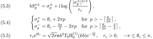
For monopole scatterers, where n = m = 0 in (3.15), equations (B.7) give the effective wavenumbersSpoat leading order:
bSpo±=σp±+ i log
|σ±
p|3/2
rc
!
, (5.3)
(
σ+
p =θc+ 2πp for p >−
θc
2π
, σ−
p =θc−3π2 −2πp for p >2πθc −34,
(5.4)
rceiθc =
√
2πnb2T0H0(1)(kb)e−i4π, r
c>0, −π≤θc≤π,
(5.5)
and for any integerp. We use the superscript “o” to distinguish these wavenumbers for monopole scatterers from others. Even though (5.4) was deduced for large integer p, it gives remarkably agreement with numerically calculated wavenumbers, except for the two lowest attenuating wavenumbers, as shown in Figure 4. In the figure we denoted So±
∗ as the effective wavenumber that can be calculated by low volume fraction expansions [26,38].
[image:14.612.71.384.488.568.2]■ ■ ■ ■ ■ ■ ■ ■ ■ ■ ■ ■ ■ ■ ■ ■ ■ ■ ▲ ▲ ▲ ▲ ▲ ▲ ▲ ▲ ▲ ▲ ▲ ▲ ▲ ▲ ▲ ▲ ▲ ▲
S*o
S1o
-S5o
-S0o+
S3o+
S7o+
■ Numeric
▲ Asymptotic
-40 -20 20 40 60
ReS 1 2 3 4 5 6 7 ImS
Fig. 4. Comparison of the asymptotic formula (5.4), which predicts an infinite number of effective wavenumbers, with numerical solutions for the effective wavenumbers(5.1). The parameters used are given by(5.2), with their definitions explained in (2.4–2.9). Here we choseb= 1.0, so the non-dimensional wavenumbersbS are the same as shown. The asymptotic formula is surprisingly accurate except for the two lowest attenuating wavenumbers. The wavenumberSo
∗ can be calculated
by using low volume fraction expansions [26].
At leading order, the asymptotic solution of (B.11) leads to the effective wavenum-bers:
bSpk± =σ±p + i log
|
σ±
p −a|
q
a|σp±|
rc , (5.6) ( σ+
p =θc+a+ 2πp for p >−θc+a2π ,
σ−
p =θc+a−3π2 −2πp for p >
θc+a 2π − 3 4 , (5.7)
rceiθc=−2inb2
∞ X
n=−∞
Tn, rc>0 and −π≤θc≤π,
(5.8)
for integerp. This confirms that there are an infinite number of effective wavenumbers for large scatterers, i.e. bk≫1. The distribution of these wavenumbers is similar to the monopole wavenumbers shown inFigure 4.
These asymptotic formulas (5.4) and (5.6) demonstrate the existence of multiple effective waves in the limit of small (monopole and Dirichlet) scatterers (5.4) and large scatterers (5.6). However, neither of these formulas, nor the low volume fraction expansions of the wavenumber [26], are able to accurately estimate the low attenuating backward travelling effective wavenumber such asS1 shown inFigure 3(in this case
not related to theS1o±andS1k±given above). There is currently no way to analytically
estimate these types of wavenumbers, even though they are necessary to accurately calculate transmission due to their small attenuation. The only approach it seems is to numerically solve (3.30).
[image:15.612.126.383.86.274.2]analytic solution with a classical method that assumes only one effective wavenum-ber [26, 29], and the Matching Method [18], recently proposed by the authors. It should be noted that all of these approaches aim to solve the same equation (2.14).
Note that for monopole scatterers, using only one effective wavenumber s1 can,
in some cases, lead to accurate results. However, for multipole scatterers (a more common scenario practically) this is rarely the case because, as shown by Figure 3, there can be at least two effective wavenumbers with low attenuation, and therefore both are needed to obtain accurate results.
For the numerical examples we use the parameters
(6.1) T0=−
J0(kao)
H(1)0 (kao)
, b= 1.001, ao= 0.5, θinc =
π
4, φ= 30%,
which implies that the number fraction n≈0.38 per unit area. When we choose to fix the wavenumber, as we do forFigure 5and6, we use bk= 1.001. This leads to a wavelength (2π/k) which is roughly six times larger than the particle diameter. If the particle was, say, more than a hundred times smaller than the wavelength, then only one effective wavenumber in the sum (4.4) would be necessary to accurately calculate A0(X).
0 1 2 3 4
0.0 0.2 0.4 0.6 0.8 1.0 1.2
x/b
|A1 0eis1x|
P352
p=1A
p
0eispx
Matching method
Low vol. frac.
0.00 0.02 0.04 0.4
0.6 0.8 1.0
x/b
Fig. 5. Compares the absolute value of the average fieldA0(x) calculated by different
meth-ods. The fieldA0(x)is closely related to the average transmitted wave [29]. The non-dimensional
wavenumber kb= 1.001, the other parameters are given by (6.1), with their definitions explained by (2.4–2.9). Using the Wiener-Hopf solution (4.4), we approximate A0(x) by using either 352
effective wavenumberss1, s2, . . . , s352, or just 1 effective wavenumbers1. The Matching Method
also accounts for multiple effective wavenumbers, and is described in [18]. The low volume fraction method assumes a low volume fraction expansion for just one effective wavenumber [26]. The small graph on the right is a magnification of the region aroundx = 0. Close to the boundary x= 0, bothA1
0e
is1x and the low volume fraction method are inaccurate, which would potentially lead to
inaccurate predictions for transmission and reflection.
To start we compare the average scattering coefficient A0(x) calculated by the
[image:16.612.99.411.336.513.2]rapid transition. The low volume fraction method is the most commonly used in the literature: it assumes a small particle volume fraction7 and just one effective wavenumber [26, 29]. One significant conclusion we can draw fromFigure 5 is that both the low volume fraction method andA1
0eis1x are inaccurate near the boundary
x= 0. This means that both of these methods lead to inaccurate reflection coefficients. In general, the Wiener-Hopf method does not lead to an explicit formula for the reflection coefficient (3.35), because we do not have an exact factorisation (3.23) for any truncated square matrices. However, there are methods [18,29, 24, 2, 5, 1] to calculate An(x), from which we can obtain the reflection coefficient (2.12). The
method [18] also accounts for multiple effective wavenumbers. So one important question is: when using (2.12), how many effective wavenumbers do we need to obtain an accurate reflection coefficient?
100.0 100.5 101.0 101.5 102.0 102.5
10−3
10−2
10−1
100
P
|RP−R| |R|
Fig. 6.Demonstrates, with a log-log graph, how increasing the number of effective wavesP leads to a more accurate reflection coefficientRP, when using (4.6). The non-dimensional wavenumber
is kb = 1.001, and the other parameters used are given by (6.1), with their definitions explained by (2.4–2.9). HereRis the reflection coefficient given by (4.5). The error|RP −R|continuously
drops asP increases because of the rapid transition that occurs toA0(x)near the boundaryx= 0,
seeFigure 5. However, methods such as the Matching Method [18] are able to accurately calculate the reflection coefficient without taking into account this rapid transition.
In Figure 6 we show how increasing the number of effective waves P reduces the error between RP (4.6) and R (4.5). To calculate a highly accurate reflection coefficientR, we could use either (4.5) or the Matching Method [18,15], as both give approximately the sameR.
Now we ask: how does the reflection coefficient (4.6), deduced via the Wiener-Hopf technique, compare with other methods across a broader range of wavenumbers. The result is shown inFigure 7, whereROis a low volume fraction expansion8 of just one effective wavenumber [29]. The reflection coefficient RM is calculated from the Matching Method [18,15]. The general trend is clear: RO becomes more inaccurate as we increase the background wavenumberkb. On the other hand bothRM andR agree closely over allk.
One result to note is the “instability“ exhibited by the Wiener-Hopf solution near the boundary x = 0, see Figure 5. This instability occurs because we represented
7For the low volume fraction method we used a small volume fraction expansion for the
wavenum-ber, but we numerically evaluated the wave amplitude. This is because the alternative, a small volume fraction expansion of the wave amplitude, led to poor results.
8We use the reflection coefficient [29, equation (39)], rather than the explicit low volume fraction
[image:17.612.162.346.250.376.2]0.5 1.0 1.5 2.0 0%
5% 10% 15% 20%
kb
|R−RO| |R|
0.5 1.0 1.5 2.0 2×10⁻⁶
3×10⁻⁶ 4×10⁻⁶ 5×10⁻⁶ 6×10⁻⁶ 7×10⁻⁶
kb
|R−RM| |R|
Fig. 7. Compares different methods for calculating the reflection coefficient when varying the non-dimensional wavenumberkb. The other parameters used are given by (6.1), with their defini-tions explained in (2.4–2.9). HereR is given by the Wiener-Hopf solution (4.5), RO uses a low volume fraction expansion of just one effective wavenumber [29], and RM is calculated from the
Matching Method [18].
A0(x) as a superposition of truncated waves, which is only accurate as long as the
discarded terms are small. So, for a truncation numberP, we can expect the instability to occur when eisPx
is not small, i.e. x ≈ 1/Imsp. However, this instability does
not affect the accuracy of the reflection coefficient (4.5) deduced by the Wiener-Hopf technique, as demonstrated by close agreement with the Matching Method inFigure 7.
7. Conclusion and Next Steps. The major result of this paper is to prove that the ensemble-averaged field in random particulate materials consists of a superposi-tion of waves, with complex effective wavenumbers, for one fixed incident wavenum-ber. These effective wavenumbers are governed by the dispersion equation (5.1). We showed asymptotically in Section 5that this has an infinite number of solutions, and hence there are an infinite number of effective wavenumbers. The Wiener-Hopf tech-nique also provides a simple and elegant expression for the reflection coefficient (3.35), whose form can be used to guide and assess methods to characterise microstruc-ture [44,17].
To numerically implement the Wiener-Hopf technique, we considered particles that scatter only in their monopole mode inSection 6. There we saw that when close to the interface of the half-space, a large number of effective wavenumbers were nec-essary to reach accurate agreement with an alternative method from the literature, the Matching Method as introduced by the authors in [18]. To obtain a constructive method via the Wiener-Hopf technique for general scatterers, and not just monopole scatterers, will require the factorisation of a matrix-function [43], which is challeng-ing. For these reasons the Matching Method [18] is presently more effective than using the Wiener-Hopf technique. However, there is ongoing work to use approximate methods [50,4,1] which exploit the symmetry and properties of the matrix (3.15).
[image:18.612.79.435.92.231.2]the solution of (2.14) with multipole methods [28, 16] in order to investigate their accuracy and limits of validity.
Appendix A. The Fourier transformed kernel ψˆn(s). Here we calculate
the Fourier transform (3.3) ofψn(X) (2.13). To do so, it is simpler to use
(A.1) Fn(X, Y) = (−1)nH(1)n (kR)einΘ.
Note that both Fn(X, Y) and ei(sX+Y ksinθinc) satisfy wave equations, with
∇2Fn(X, Y) =−k2Fn(X, Y) and ∇2ei(sX+Y ksinθinc)=−S2ei(sX+Y ksinθinc),
where we used (2.13)2 for the first equation and (3.19) for the second equation. This
means that we can use Green’s second identity to obtain
(A.2) (k2−S2)
ˆ
B
ei(sX+Y ksinθinc)F
n(X, Y)dXdY
=
ˆ
∂B
∂ei(sX+Y Ksinθinc)
∂n Fn(X, Y)−e
i(sX+KYsinθinc)∂Fn(X, Y) ∂n
dz,
for any areaB in which the integrand is analytic, where nis the outwards pointing unit normal and dzis a differential length along the boundary∂B. To calculate ˆψn(s),
the regionB becomes R ≥b, with (R,Θ) being the polar coordinates of (X, Y), in which case the integral overBconverges because asR→ ∞we have that
(A.3) |ei(sX+Y ksinθinc)F
n(X, Y)| ∼|
eisRcos ΘeikR(1+sin Θ sinθinc)| p
π|k|R/2
≤ |e
−R(Imk(1−|sinθinc|)−|Im (s)|)| p
π|k|R/2 →0,
exponentially fast when|Im (s)|<Imk(1− |sinθinc|). Under this restriction, and by
assumingS6=±k, (A.2) then leads to
(A.4) ψˆn(s) = ˆ
R≥b
eisX+ikYsinθincF
n(X, Y)dXdY = In(b)
k2−S2,
by usingsX+Y ksinθinc=RScos(θ−θS) from (3.19) and
(A.5) In(R) = ˆ 2π
0 −
∂eiSRcos(Θ−θS)
∂R Fn(kX) + e
iSRcos(Θ−θS)∂Fn(kX)
∂R RdΘ
= (−1)n ˆ 2π
0
eiSRcos(Θ−θS)einΘkH(1)′
n (kR)−iScos(Θ−θS)H(1)n (kR)
Rdθ
= (−1)n
ˆ 2π
0
∞ X
m=−∞
imJm(SR)eim(Θ−θS)
h
keinΘH(1)n ′(kR)
−i2S(ei(n+1)Θ−iθS+ ei(n−1)Θ+iθS)H(1)n (kR)
i
RdΘ
= 2π(−i)nReinθS
h
kJn(SR)H(1)n ′(kR)−SJ′n(SR)H(1)n (kR)
i
where Jnis the Bessel function of the first kind, and we used the Jacobi-Anger
expan-sion on eiSRcos(Θ−θS), integrated over Θ and used the identity J
n−1(SR)−Jn+1(SR) =
2J′
n(SR). In summary
(A.6) ψˆn(s) = 2π
(−i)neinθS
α2−s2 Nn(bS),
when the condition (3.10) is satisfied, with Nn given by (3.17).
Below we establish some useful properties for ˆψn(s). In particular, we show that
ˆ
ψn(s) has no branch-points.
The function Nn(bS) can be expanded aroundS= 0 as
(A.7) Nn(bS) = (−1)nS|n|
∞ X
m=0
cmS2m,
where thecmare some constants, and the radius of convergence of the series above is
infinite. Using (3.19) we can write (A.8)
einθS = ei sgn(n)|n|θS = (cosθS+ sgn(n)i sinθS)|n|= (s+ sgn(n)iksinθinc)|n|S−|n|.
Substituting (A.7) and (A.8) in (A.6) results in
(A.9) ψˆn(s) =
2πin
α2−s2(s+ sgn(n)iksinθinc)
|n| ∞ X
m=0
cmS2m.
BecauseS2=s2+k2sin2θ
inc, we can see from the above that ˆψn(s) has no
branch-points. From the above, we can also establish the properties:
(A.10) ψˆn(s) = ˆψ−n(−s) = ˆψn(−s)e2inθS(−1)n.
Appendix B. Asymptotic wavenumbers. Here we explicitly calculate a sequence of effective wavenumbersSp, assuming|Sp|large and increasing withp, and
ImSp>0, a that asymptotically satisfy (5.1). A key step is to approximate the terms
appearing in (3.16), such as
(B.1) Jn(bS)∼
eiπ4+ inπ
2 −ibS √
2πbS and J ′
n(bS)∼
e−iπ
4+ inπ
2 −ibS √
2πbS ,
for large|bS|, where the terms eibS are discarded as ImbS→ ∞.
Monopole scatterers. The simplest case is for monopole scatterers, where n = m= 0 in (3.16), and the effective wavenumber S satisfies
(B.2) b2detG= (bS)2−(bk)2+ 2πnb2T0N0(bS)∼(bS)2−c√bSe−ibS= 0,
wherec=√2πnb2T0H(1) 0 (kb)e−
iπ
4. Here we used (B.1), and ignored terms which are algebraically smaller thanbS. To find the root of the above we substitute
(B.3) bS=x+ i logy,
wherexandy are real, and|x|andy are large withy >1. This leads to
For the logarithm and square root we use the typical branch cut (−∞,0) and take positive values of the functions for positive arguments. For the above to be satisfied to leading order thenx3/2∼y, which reduces the above equation to
(B.5) x3/2∼rcei(θc−x)y,
where we substituted c = rceiθc, for real scalars rc and θc. Equating the real and
imaginary parts of the above leads to
x∼θc+ 2πp and y∼ 1
rc
(θc+ 2πp)3/2 for p >−θc
2π (B.6)
x∼θc−3π
2 + 2πp and y∼ 1
rc(−θc+
3π 2 −2πp)
3/2 for p < 3
4 − θc
2π, (B.7)
for integersp. From this we can identify that, at leading order, the effective wavenum-bers are given by (5.4).
Multipole scatterers:. With the same method used above, we can also demonstrate the existence of multiple effective wavenumbers for n, m = −M,−M + 1,· · · , M in (3.16). To show this explicitly, we consider bk to be the same order asbS, that is |k| ∼ |S|.
By consideringbklarge, we can approximate
(B.8) H(1)n (bk)∼ei(bk− π
4−
nπ
2 ) r
2
πbk and H
(1)′
n (bk)∼ei(bk+ π
4−nπ2 ) r
2 πbk,
combining this with (B.1) and considering|k| ∼ |S|, the term (3.16) at leading order becomes
(B.9) b2G
mn=d0δmn+c0Tm,
where
d0= (bS)2−(bk)2, and c0= 2nb2i(k√+S)
kS e
ib(k−S).
By simple rearrangement of the determinant we find that9
(B.10) det(b2G) =d2M0 d0+c0 M
X
m=−M
Tm
!
.
Note thatd06= 0, i.e.S 6=±k, was necessary to reach the condition (3.10), which was
used to calculate the Fourier transforms (3.13). Taking this into consideration, and taking the limitM → ∞, the effective wavenumbersS must satisfy
(B.11) d0+c0 M
X
m=−M
Tm= 0 =⇒ bS−bk=−2nib2
∞ X
m=−∞ Tm
eib(k−S)
b√kS .
Using an asymptotic expansion analogous to (B.3), the above leads to the effective wavenumbers (5.6).
Appendix C. Equivalent determinants. For any square matricesAandB, and scalarc, ifAnm=Bnmcn−m, then
(C.1) detA= detB,
9The determinant ofb2Gequals the product of its eigenvalues. The eigenvector (T
which follows from defining the diagonal matrix Cnm =δnmcn, thenA=CBC−1,
and det(CBC−1) = detCdetBdetC−1= detB.
REFERENCES
[1] I. D. Abrahams,Scattering of sound by two parallel semi-infinite screens, Wave Motion, 9 (1987), pp. 289–300,https://doi.org/10.1016/0165-2125(87)90002-3.
[2] I. D. Abrahams, Radiation and scattering of waves on an elastic half-space; A non-commutative matrix Wiener-Hopf problem, Journal of the Mechanics and Physics of Solids, 44 (1996), pp. 2125–2154,https://doi.org/10.1016/S0022-5096(96)00064-6.
[3] I. D. Abrahams,On the Solution of Wiener–Hopf Problems Involving Noncommutative Matrix Kernel Decompositions, SIAM Journal on Applied Mathematics, 57 (1997), pp. 541–567,
https://doi.org/10.1137/S0036139995287673.
[4] I. D. Abrahams, The application of Pad approximants to Wiener-Hopf factorization, IMA Journal of Applied Mathematics, 65 (2000), pp. 257–281,https://doi.org/10.1093/imamat/ 65.3.257.
[5] I. D. Abrahams and G. R. Wickham,General WienerHopf Factorization of Matrix Ker-nels with Exponential Phase Factors, SIAM Journal on Applied Mathematics, 50 (1990), pp. 819–838,https://doi.org/10.1137/0150047.
[6] M. Albani and F. Capolino,Wave dynamics by a plane wave on a half-space metamaterial made of plasmonic nanospheres: a discrete WienerHopf formulation, JOSA B, 28 (2011), pp. 2174–2185,https://doi.org/10.1364/JOSAB.28.002174.
[7] N. Bleistein and R. A. Handelsman,Asymptotic expansions of integrals, Courier Corpora-tion, 1986.
[8] J.-M. Conoir and A. N. Norris, Effective wavenumbers and reflection coefficients for an elastic medium containing random configurations of cylindrical scatterers, Wave Motion, 47 (2010), pp. 183–197,https://doi.org/10.1016/j.wavemoti.2009.09.004.
[9] D. G. Crighton, A. Dowling, J. Ffowcs Williams, M. Heckl, and F. Leppington,Modern Methods in Analytical Acoustics, Springer-Verlag, 1992.
[10] J. G. Fikioris and P. C. Waterman,Multiple Scattering of Waves. II. “Hole Corrections” in the Scalar Case, Journal of Mathematical Physics, 5 (1964), pp. 1413–1420, https: //doi.org/10.1063/1.1704077.
[11] L. L. Foldy,The multiple scattering of waves. I. General theory of isotropic scattering by randomly distributed scatterers, Physical Review, 67 (1945), p. 107.
[12] M. Ganesh and S. C. Hawkins,A far-field based T-matrix method for two dimensional obstacle scattering, ANZIAM Journal, 51 (2010), pp. 215–230.
[13] M. Ganesh and S. C. Hawkins,Algorithm 975: TMATROMA T-Matrix Reduced Order Model Software, ACM Trans. Math. Softw., 44 (2017), pp. 9:1–9:18, https://doi.org/10.1145/ 3054945.
[14] I. C. Gokhberg and M. G. Krein,Systems of integral equations on the half-line with kernels depending on the difference of the arguments, 14 (1960), pp. 217 – 287.
[15] A. L. Gower,EffectiveWaves.jl: A package to calculate ensemble averaged waves in heteroge-neous materials., https://github.com/arturgower/EffectiveWaves.jl/tree/v0.2.0 (accessed 2018-24-10).https://github.com/arturgower/EffectiveWaves.jl/tree/v0.2.0.
[16] A. L. Gower and J. Deakin,MultipleScattering.jl: A Julia library for simulating, process-ing, and plotting multiple scattering of acoustic waves., 2018,https://github.com/jondea/ MultipleScattering.jl(accessed 2017-12-29). original-date: 2017-07-10T10:06:59Z. [17] A. L. Gower, R. M. Gower, J. Deakin, W. J. Parnell, and I. D. Abrahams,Characterising
particulate random media from near-surface backscattering: A machine learning approach to predict particle size and concentration, EPL (Europhysics Letters), 122 (2018), p. 54001. [18] A. L. Gower, W. J. Parnell, and I. D. Abrahams,Multiple Waves Propagate in Random
Particulate Materials, arXiv:1810.10816 [physics], (2018). arXiv: 1810.10816.
[19] A. L. Gower, M. J. A. Smith, W. J. Parnell, and I. D. Abrahams, Reflection from a multi-species material and its transmitted effective wavenumber, Proc. R. Soc. A, 474 (2018), p. 20170864,https://doi.org/10.1098/rspa.2017.0864.
[20] S. G. Haslinger, I. S. Jones, N. V. Movchan, and A. B. Movchan,Semi-infinite herring-bone waveguides in elastic plates, arXiv:1712.01827 [physics], (2017). arXiv: 1712.01827. [21] S. G. Haslinger, N. V. Movchan, A. B. Movchan, I. S. Jones, and R. V. Craster,
Controlling flexural waves in semi-infinite platonic crystals, arXiv:1609.02787 [physics], (2016). arXiv: 1609.02787.
Factors, SIAM Journal on Applied Mathematics, 78 (2018), pp. 45–62,https://doi.org/10. 1137/17M1136304.
[23] G. Kristensson,Coherent scattering by a collection of randomly located obstacles An alter-native integral equation formulation, Journal of Quantitative Spectroscopy and Radiative Transfer, 164 (2015), pp. 97–108,https://doi.org/10.1016/j.jqsrt.2015.06.004.
[24] J. B. Lawrie and I. D. Abrahams,A brief historical perspective of the WienerHopf technique, Journal of Engineering Mathematics, 59 (2007), pp. 351–358, https://doi.org/10.1007/ s10665-007-9195-x.
[25] M. Lax,Multiple Scattering of Waves, Reviews of Modern Physics, 23 (1951), pp. 287–310,
https://doi.org/10.1103/RevModPhys.23.287.
[26] C. M. Linton and P. A. Martin, Multiple scattering by random configurations of circu-lar cylinders: Second-order corrections for the effective wavenumber, The Journal of the Acoustical Society of America, 117 (2005), p. 3413,https://doi.org/10.1121/1.1904270. [27] C. M. Linton and P. A. Martin, Multiple Scattering by Multiple Spheres: A New Proof
of the Lloyd–Berry Formula for the Effective Wavenumber, SIAM Journal on Applied Mathematics, 66 (2006), pp. 1649–1668,https://doi.org/10.1137/050636401.
[28] P. A. Martin, Multiple Scattering: Interaction of Time-Harmonic Waves with N Obstacles, Cambridge University Press, Cambridge, 2006, https://doi.org/10.1017/ CBO9780511735110.
[29] P. A. Martin,Multiple scattering by random configurations of circular cylinders: Reflection, transmission, and effective interface conditions, The Journal of the Acoustical Society of America, 129 (2011), pp. 1685–1695,https://doi.org/10.1121/1.3546098.
[30] P. A. Martin, I. D. Abrahams, and W. J. Parnell,One-dimensional reflection by a semi-infinite periodic row of scatterers, Wave Motion, 58 (2015), pp. 1–12,https://doi.org/10. 1016/j.wavemoti.2015.06.005.
[31] P. A. Martin and A. Maurel,Multiple scattering by random configurations of circular cylin-ders: Weak scattering without closure assumptions, Wave Motion, 45 (2008), pp. 865–880,
https://doi.org/10.1016/j.wavemoti.2008.03.004.
[32] M. I. Mishchenko,Light scattering by randomly oriented axially symmetric particles, JOSA A, 8 (1991), pp. 871–882,https://doi.org/10.1364/JOSAA.8.000871.
[33] M. I. Mishchenko, Light scattering by sizeshape distributions of randomly oriented axially symmetric particles of a size comparable to a wavelength, Applied Optics, 32 (1993), pp. 4652–4666,https://doi.org/10.1364/AO.32.004652.
[34] M. I. Mishchenko, J. M. Dlugach, M. A. Yurkin, L. Bi, B. Cairns, L. Liu, R. L. Panetta, L. D. Travis, P. Yang, and N. T. Zakharova,First-principles modeling of electromag-netic scattering by discrete and discretely heterogeneous random media, Physics Reports, 632 (2016), pp. 1–75,https://doi.org/10.1016/j.physrep.2016.04.002. arXiv: 1605.06452. [35] M. I. Mishchenko, L. D. Travis, and A. A. Lacis,Multiple Scattering of Light by Particles:
Radiative Transfer and Coherent Backscattering, Cambridge University Press, 2006. [36] B. Noble,Methods Based on the Wiener-Hopf Technique., vol. 67, American Mathematical
Society, 2nd unexpurgated edition ed., July 1988.
[37] A. Norris and G. R. Wickham,Acoustic diffraction from the junction of two flat plates, Proceedings of the Royal Society of London. Series A: Mathematical and Physical Sciences, 451 (1995), pp. 631–655,https://doi.org/10.1098/rspa.1995.0147.
[38] A. N. Norris and J.-M. Conoir,Multiple scattering by cylinders immersed in fluid: High order approximations for the effective wavenumbers, The Journal of the Acoustical Society of America, 129 (2011), pp. 104–113,https://doi.org/10.1121/1.3504711.
[39] A. N. Norris, F. Lupp, and J.-M. Conoir,Effective wave numbers for thermo-viscoelastic media containing random configurations of spherical scatterers, The Journal of the Acous-tical Society of America, 131 (2012), pp. 1113–1120.
[40] W. J. Parnell and I. D. Abrahams, Multiple point scattering to determine the effective wavenumber and effective material properties of an inhomogeneous slab, Waves in Ran-dom and Complex Media, 20 (2010), pp. 678–701,https://doi.org/10.1080/17455030.2010. 510858.
[41] W. J. Parnell, I. D. Abrahams, and P. R. Brazier-Smith,Effective Properties of a Com-posite Half-Space: Exploring the Relationship Between Homogenization and Multiple-Scattering Theories, The Quarterly Journal of Mechanics and Applied Mathematics, 63 (2010), pp. 145–175,https://doi.org/10.1093/qjmam/hbq002.
[42] V. J. Pinfield and R. E. Challis, Emergence of the coherent reflected field for a single realisation of spherical scatterer locations in a solid matrix, Journal of Physics: Conference Series, 457 (2013), p. 012009,https://doi.org/10.1088/1742-6596/457/1/012009.
IMA Journal of Applied Mathematics, 81 (2016), pp. 365–391,https://doi.org/10.1093/ imamat/hxv038.
[44] R. Roncen, Z. E. A. Fellah, F. Simon, E. Piot, M. Fellah, E. Ogam, and C. Depollier,
Bayesian inference for the ultrasonic characterization of rigid porous materials using re-flected waves by the first interface, The Journal of the Acoustical Society of America, 144 (2018), pp. 210–221,https://doi.org/10.1121/1.5044423.
[45] V. P. Tishkovets, E. V. Petrova, and M. I. Mishchenko,Scattering of electromagnetic waves by ensembles of particles and discrete random media, Journal of Quantitative Spec-troscopy and Radiative Transfer, 112 (2011), pp. 2095–2127, https://doi.org/10.1016/j. jqsrt.2011.04.010.
[46] L. Tsang, C. T. Chen, A. T. C. Chang, J. Guo, and K. H. Ding, Dense media radia-tive transfer theory based on quasicrystalline approximation with applications to pas-sive microwave remote sensing of snow, Radio Science, 35 (2000), pp. 731–749, https: //doi.org/10.1029/1999RS002270.
[47] L. Tsang and A. Ishimaru,Radiative Wave Equations for Vector Electromagnetic Propagation in Dense Nontenuous Media, Journal of Electromagnetic Waves and Applications, 1 (1987), pp. 59–72,https://doi.org/10.1163/156939387X00090.
[48] L. Tsang and J. A. Kong,Scattering of electromagnetic waves from a half space of densely distributed dielectric scatterers, Radio Science, 18 (1983), pp. 1260–1272,https://doi.org/ 10.1029/RS018i006p01260.
[49] N. Tymis and I. Thompson,Scattering by a semi-infinite lattice and the excitation of Bloch waves, The Quarterly Journal of Mechanics and Applied Mathematics, 67 (2014), pp. 469– 503,https://doi.org/10.1093/qjmam/hbu014.
[50] B. H. Veitch and I. D. Abrahams,On the commutative factorization of nn matrix Wiener-Hopf kernels with distinct eigenvalues, Proceedings of the Royal Society A: Mathematical, Physical and Engineering Sciences, 463 (2007), pp. 613–639,https://doi.org/10.1098/rspa. 2006.1780.