FOR VIEWING HIGH DYNAMIC RANGE PANORAMAS
ON HEAD MOUNTED DISPLAY
by
Yuan Li
A thesis
submitted in partial fulfillment
of the requirements for the degree of Master of Science in Computer Science
Boise State University
c
2017 Yuan Li
DEFENSE COMMITTEE AND FINAL READING APPROVALS
of the thesis submitted by
Yuan Li
Thesis Title: Editable View Optimized Tone Mapping For Viewing High Dynamic Range Panoramas On Head Mounted Display
Date of Final Oral Examination: 30th June 2017
The following individuals read and discussed the thesis submitted by student Yuan Li, and they evaluated the presentation and response to questions during the final oral examination. They found that the student passed the final oral examination.
Steven Cutchin, Ph.D. Chair, Supervisory Committee
Jerry Alan Fails, Ph.D. Member, Supervisory Committee
Amit Jain, Ph.D. Member, Supervisory Committee
Maria Soledad Pera, Ph.D. Member, Supervisory Committee
dedicated to my family
I would first like to thank my thesis advisor Professor Steven Cutchin of the
Computer Science Department at Boise State University. The door to Prof. Cutchin’s
office was always open whenever I ran into a trouble spot or had a question about
my research or writing. He consistently allowed this paper to be my own work, but steered me in the right direction whenever he thought I needed it.
I would also like to thank the participants who were involved in the user survey
for this research project. Without their passionate participation and input, the user
survey could not have been successfully conducted.
I would also like to acknowledge Professor Jerry Alan Fails of the Computer
Sci-ence Department at Boise State University for his very valuable advice on conducting
user study.
Finally, I must express my very profound gratitude to my family for providing me
with unfailing support and continuous encouragement throughout my years of study
and through the process of researching and writing this thesis. This accomplishment
would not have been possible without them. Thank you.
ABSTRACT
Head mounted displays are characterized by relatively low resolution and low
dynamic range. These limitations significantly reduce the visual quality of
photore-alistic captures on such displays. This thesis presents an interactive view optimized
tone mapping technique for viewing large sized high dynamic range panoramas up to 16384 by 8192 on head mounted displays. This technique generates a separate
file storing pre-computed view-adjusted mapping function parameters. We define
this technique as ToneTexture. The use of view adjusted tone mapping allows for expansion of the perceived color space available to the end user. This yields an
improved visual appearance of both high dynamic range panoramas and low dynamic
range panoramas on such displays. Moreover, by providing proper interface to
ma-nipulate on ToneTexture, users are allowed to adjust the mapping function as to changing color emphasis. The authors present comparisons of the results produced
byToneTexture technique against widely-used Reinhard tone mapping operator and Filmic tone mapping operator both objectively via mathmatical quality assessment
metrics and subjectively through user study. Demonstration systems are available for
desktop and head mounted displays such as Oculus Rift and GearVR.
ABSTRACT . . . vi
LIST OF TABLES . . . x
LIST OF FIGURES . . . xi
LIST OF ABBREVIATIONS . . . xiv
LIST OF SYMBOLS . . . xvi
1 Introduction . . . 1
1.1 High Dynamic Range Imagery . . . 1
1.2 Tone Mapping . . . 3
1.3 Related Work . . . 5
1.4 Thesis Statement . . . 9
2 Methodology . . . 13
2.1 Equirectangular Projection . . . 14
2.2 Tone Mapping Function . . . 21
2.2.1 Luminance Histogram and Bernstein Curve . . . 21
2.2.2 Cubic Spline . . . 28
3 Implementations . . . 35
3.1 Viewing Window Capture . . . 36
3.2 Cubic Spline Coefficients . . . 41
3.3 Editing Interface . . . 45
3.4 Implemented Demos . . . 50
3.4.1 Spheres and Cubes . . . 51
3.4.2 Texture Tiling . . . 53
3.4.3 HDR Encoding . . . 55
4 Results . . . 58
4.1 User Evaluation . . . 66
4.1.1 Parameters . . . 66
4.1.2 Results . . . 68
4.2 Objective Quality Assessment . . . 75
4.2.1 TMQI . . . 75
4.2.2 Analysis . . . 77
5 Conclusion and Future Work . . . 89
5.1 Conclusion . . . 89
5.2 Future Work . . . 90
BIBLIOGRAPHY . . . 92
A Asynchronous Pixel Reading Implementation . . . 96
B Tridiagonal Matrix Algorithm . . . 98
C Evaluation Dataset . . . 102
C.1 Task 1 . . . 103
C.2 Task 3 . . . 104
LIST OF TABLES
3.1 Camera Configuration . . . 35
3.2 Half Precision Bits Conversion . . . 57
4.1 Panorama Luminance Information . . . 60
C.1 Data-set From User Evaluation Task 1 . . . 103
C.2 Data-set From User Evaluation Task 3 . . . 104
C.3 Data-set From TMQI . . . 107
1.1 Screen Door Effect . . . 2
1.2 Tone Mapping Effects . . . 3
1.3 Viewer Location Example . . . 4
1.4 Fast Bilateral Filtering . . . 5
1.5 Gradient Domain HDR Compression . . . 6
1.6 Slim Backlight Drive . . . 7
1.7 Naughty Dog Filmic Example . . . 9
1.8 Spline Interpolation . . . 10
2.1 Equirectangular Panorama Example . . . 14
2.2 Equirectangular Project Distortion . . . 16
2.3 View Angle Effects . . . 17
2.4 Incorrect Window Identification . . . 18
2.5 Capture Program Setup . . . 20
2.6 Histogram Processing Using Bernstein Polynomial . . . 26
2.7 Cubic Spline Example . . . 29
2.8 Boundary Constraints Effects . . . 32
3.1 Asynchronous Reading Flow . . . 37
3.2 Filmic Curve Components . . . 46
3.3 Filmic Curve Toe . . . 47
3.4 Panorama Viewer Architecture . . . 50
3.5 Cubemap Illustration . . . 51
3.6 Cubemap Transformation . . . 53
3.7 Texture Tiling . . . 55
3.8 HDR Encoding . . . 56
4.1 Tone Mapping Effects . . . 61
4.2 Histograms of original HDR High region and tone mapped images correspond to the first row in Figure 4.1 . . . 62
4.3 Histograms of original HDR Low region and tone mapped images correspond to the second row in Figure 4.1 . . . 63
4.4 Histograms of original HDR Mid region and tone mapped images correspond to the third row in Figure 4.1 . . . 64
4.5 Histograms of original HDR High&Low region and tone mapped images correspond to the last row in Figure 4.1 . . . 65
4.6 User Preference by Region in Task 1 . . . 70
4.7 User Preference by Panorama in Task 1 . . . 71
4.8 Tone Mapping Effects in Task 3 . . . 72
4.9 User Preference by Region in Task 3 . . . 74
4.10 User Preference by Panorama in Task 3 . . . 75
4.11 TMQI: Q Score . . . 79
4.12 TMQI: Q Score(continued) . . . 80
4.13 TMQI: S Score . . . 83
4.14 TMQI: S Score(continued) . . . 84
4.15 TMQI: N Score . . . 87
A.1 Asynchronous Pixel Data Reading Code . . . 97
LIST OF ABBREVIATIONS
API– Application Programming Interface
CPU – Central Processing Unit
DMA – Direct Memory Access
FBO – Frame Buffer Object
FOV – Field Of View
FPS – Frames Per Second
GPU – Graphics Processing Unit
HDR – High Dynamic Range
HMD – Head Mounted Display
HVS – Human Visual System
LDR– Low Dynamic Range
MPI – Message Passing Interface
OpenCV – Open Source Computer Vision Library
OpenGL – Open Graphics Library
PBO – Pixel Buffer Object
SDR – Standard Dynamic Range, equivalent to LDR
TMO – Tone Mapping Operator
VR – Virtual Reality
LIST OF SYMBOLS
√
2 square root of 2
λ longitude on the spherical surface.
ϕ latitude on the spherical surface.
CHAPTER 1
INTRODUCTION
1.1
High Dynamic Range Imagery
With current virtual reality (VR) popularity, head mounted displays (HMD) are
becoming widely available. These devices can be desktop-oriented headsets like
Oculus Rift and HTC Vive, or small goggles that can turn into an immersive VR
HMD after connecting to your cell phone.
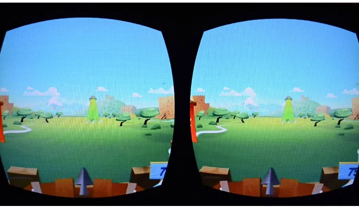
Current HMDs have a severe screen door effect, a visual artifact of the display
devices where the fine lines between pixels (or subpixels) are visible in the displayed
image. This is caused by the close distance between the display screen and the viewer’s
eye, the use of magnifying lenses to increase field of view [38] and the insufficient pixel
density of the device [2, 21]. This combined with their low dynamic range display ability leads to a notably reduced visual quality under the device resolution [33]. As
illustrated in Figure 1.1.
Given the fact that the screen resolution can not be easily increased, an alternative
avenue for improving visual quality is to introduce high dynamic range (HDR) imagery
to provide better image quality in terms of color space. However, most display
monitors and HMDs have a limited color range display ability that only supports low
dynamic range (LDR) imagery [6]. The term “dynamic range” is used to describe the
2
Figure 1.1: Screen door effects on HTC Vive VR headset
The most widely used standard dynamic range (SDR) or LDR has 256 distinct degrees
of luminance since each pixel is stored in 8-bit integers. Compared to what we perceive
everyday, this is a dynamic range too narrow to represent real world scenes. HDR
imagery, on the other hand, uses floating point numbers to represent pixel values and
therefore can reproduce a far greater dynamic range of luminosity. If the image uses a 32-bit single precision floating point number, the dynamic range will have up to 232 divisions in brightness as there are 232 different binary combinations. Broad dynamic range like this can present a similar range of luminance to that experienced through
the human visual system (HVS), such as many real-world scenes containing both very
bright, direct sunlight and extreme dim shade [4]. In conclusion, HDR means more
(a) Simple contrast reduction (b) Filmic Tone Mapping
Figure 1.2: Two resulting tone mapped images generated by different tone mapping operators
1.2
Tone Mapping
Due to the limitations of display contrast, the extended luminosity range of an HDR image has to be compressed to be made visible. The technique to map one set of
colors to a smaller one to approximate the appearance of HDR images in a medium
that has a more limited dynamic range is called tone mapping. This method reduces
the overall contrast of an HDR image to facilitate display on devices with lower
dynamic range display ability, and can be applied to produce images with preserved
local contrast or exaggerated for artistic effect. Tone mapping addresses the problem
of severe contrast reduction from original scene radiance to the target displayable range while preserving the image details and color appearance that are important to
appreciate scene content, as shown in Figure 1.2. Because of the reduction in dynamic
range, tone mapping inevitably causes information loss [23, 24, 40, 41].
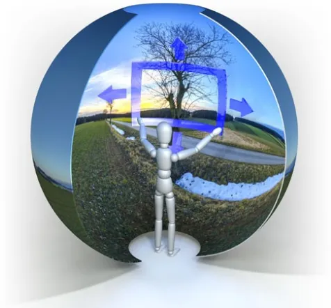
When viewing a panorama image via HMD, the user only sees a small region of
the entire panorama at a particular moment, as illustrated in Figure 1.3. This means
4
Figure 1.3: User viewing spherical panorama when located at the center
when a user tries to view an HDR panorama where range of luminance levels is on
the order of 10,000 to 1 [28], a global tone mapping operator (TMO) is applied to
the entire image. The resulting LDR panorama will have a much narrower luminance
range throughout the whole image, normally from 0 to 255. This means that the user, who is only able to see a small region out of the entire panorama, will end up
looking at a viewport where luminance range is even narrower than that of the LDR
panorama. Therefore visual quality for the end user can be significantly improved by
just applying tone mapping on the HDR pixels within the current viewable rectangle.
In this way, every small region the user views can utilize the available 256 shades of
Figure 1.4: Fast bilateral filtering for the display of high-dynamic-range images by Frdo Durand and Julie Dorsey
1.3
Related Work
There have been related works in localized TMOs over the past decade [12, 13, 32].
Many of them focus on optimizing viewing quality in local regions of high contrast
scenes. The mapping function used in these local operators varies spatially, depending
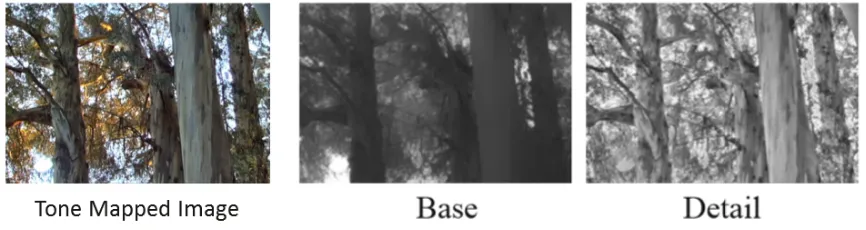
on the neighborhood of the pixel. Fr´edo Durand and Julie Dorsey use a fast bilateral
filtering to extract two layers from the input HDR image - the base layer which only
consists of large-scale variations and the detail layer created via dividing input image’s
intensity by the base layer [12]. Then contrast reduction is only applied to the base layer so that details from the input HDR image are preserved as much as possible.
The decomposed layers as well as a tone mapped LDR image is shown in Figure 1.4.
The work done by Raanan Fattal, Dani Lischinski and Michael Werman
intro-duced a conceptually simple, computationally efficient and robust tone mapping
method [13]. Instead of directly modify on the luminosity, their focus is on the
gradient field of the input HDR image. Their TMO begins by attenuating large
gradients in the original field and then constructs an globally optimized LDR image
6
Figure 1.5: Gradient Domain High Dynamic Range Compression by Raanan Fattal, Dani Lischinski and Michael Werman. The darker shade in the attenuation factor map indicates stronger attenuation
work, this TMO demonstrates that it is capable of drastic dynamic range compression,
while preserving fine details and avoiding common artifacts, such as halos, gradient
reversals, or loss of local contrast. The method is also able to significantly enhance
ordinary images by bringing out detail in dark regions. Figure 1.5 provides the
gradient attenuation factor map generated from an HDR input image using this TMO and the final tone mapped LDR image.
In [32], the authors presented a window-based tone mapping method that uses
a linear function to constrain the tone reproduction inside predefined overlapping
windows in order to naturally suppress strong edges while retaining weak ones. Then
the HDR image is tone mapped by solving an image-level optimization problem
that integrates all windows-based constraints. And it is generally noticed that local operators, which reproduce the tonal values in a spatially variant manner, perform
more satisfactorily than global operators.
Even though these methods all generate LDR images with good visual quality
while preserving contrast details, they have fundamental limitations to be applied to
output. No matter how good these resulting LDR images are, they cannot exploit
as many levels of available luminance as possible, considering the user is only able to
see a small portion of the whole image. Moreover, computationally efficient as these methods are, they are still too expensive to run in real time. That is to say, even
when applying these methods just to the small viewable region, the computational
cost will severely jeopardize the application’s frame rate. When the user is exposed
to an immersive VR environment, insufficient frame rate is one of the major causes of
virtual reality sickness [22], a term for symptoms that are similar to motion sickness
symptoms like general discomfort, headache, stomach awareness, nausea, vomiting,
pallor, sweating, fatigue, drowsiness, disorientation, and apathy [20]. Computational
cost combined with hardware limitation makes these methods not ideal while using HMD as the display media.
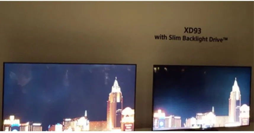
Figure 1.6: Slim Backlight Drive on Sony’s new commercial HDR TVs that allows localized illumination based on image content
8
found in Sony’s Slim Backlight Drive technology on the company’s new commercial HDR TVs, as illustrated in Figure 1.6. Note that these commercial HDR TVs only
use extended integers for pixel luminance representation instead of floating point numbers. While they do possess a more extended dynamic range than traditional
LDR TVs, the produced luminosity range is still no match for true HDR. Introduced
for the first time in early 2016, this new technology aims to provide the best of both
worlds between the slim aesthetics of edge-lit LEDs, and more precise local dimming
allowed by direct-lit FALD sets. Sony wont go into much technical detail on how the Slim Backlight Drive works, other than to say that its based on a grid lighting approach that allows edge LED lighting to illuminate relatively small sectors within
the image independently of each other, rather than just being able to control top to bottom or left to right strips of the image as has been the case previously.
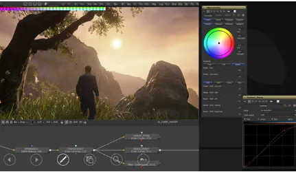
There hasn’t been much work in tone mapping editing. Video game developing
companyNaughty Dog creates and uses an adaptive Filmic TMO in their latest game
Uncharted4 to render a massive amount of HDR resources [14]. The developers first introduce a look-up table for tone mapping parameters for the Filmic curve. Then a
graphical interface is designed to allow game artists to dynamically adjust different sections of this Filmic curve. Modification can be observed immediately after artists
finish editing. This live update also enables the artists to freely look around the scene
as they are tweaking colors to make sure the curve creates beautiful views everywhere,
as shown in Figure 1.7. This technique is still aiming for a global view optimization
whereas our proposed method optimizes visible content on sub-region scales while
Figure 1.7: Artist adjusted tone mapping curve in Uncharted 4
1.4
Thesis Statement
This thesis presents a novel technique that not only supports view optimized tone
mapping of high resolution (up to 16384 by 8192 in pixels) photographic HDR
panora-mas, but also allows for real-time tone mapping editing to dynamically adjusting
col-oring emphasis. This technique is defined asToneTexture, named after the generated extra texture file that stores pre-computed tone mapping parameters. The Tone-Texture technique features dynamic tone mapping of an HDR panorama customized to the view direction of the user. This method applies a TMO customized to the
panorama content that is visible to the user based on current view direction while
also utilizing both global and regional panorama image luminance details to maintain
a consistent coloring of the resulting LDR panorama in whatever direction the user
10
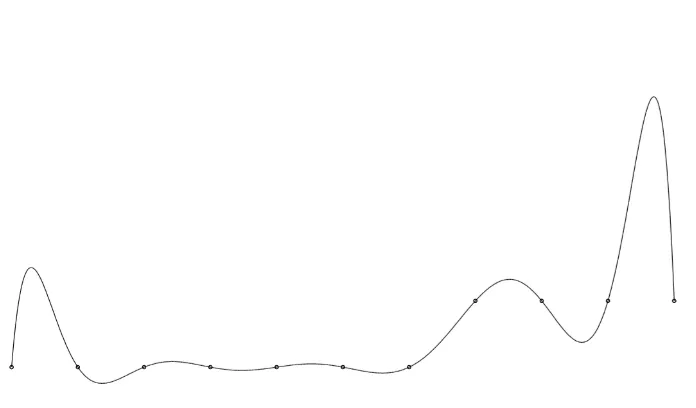
Figure 1.8: Cubic spline interpolation of 11 data points
ToneTexture can utilize a variety of TMOs as determined to most optimally work for selected content. The implementation presented in the thesis combines the use of cubic spline functions with window-based image processing. The method
is conceptually simple yet efficient, flexible and robust. By associating a window
region to every possible view angle on the panoramic sphere, localized optimization
can be achieved while covering the entire HDR panorama image. To assure real-time
viewing performance,ToneTexturetechnique allocates most computational operations in pre-processing phase. The results - cubic spline function coefficients - are then
stored in an extra texture file which is referred to as ToneTexture.
The reason for adopting cubic splines as TMO is because their curve shapes can be
modified directly by manipulating on the control points [5]. For a piecewise smooth cubic spline, the shape is only determined by the knots1 [30]. By modifying one knot’s Y value, it can generate a high peak or a low trough on the curve. Likewise,
by adjusting one knot’s X value, the newly generated peak or trough can be shifted
in theX axis accordingly, as shown in Figure 1.8. In this way, the cubic spline
tion grants the ToneTexture technique enough control while also ensuring flexibility and robustness to handle windows of various luminance distributions. Notably, it
is not optimal to allow the artists to manipulate on all knots directly when they are immersed in the virtual scene via HMD. This thesis addresses this problem by
developing an user-friendly interface that groups modification on knots from different
luminance regions like bright regions and dim regions so that users can adjust coloring
emphasis intuitively and easily.
Apart from the interface, another issue resolved for both viewing and editing
functionalities is the smoothing of tone mapping parameters. SinceToneTexture only considers local luminance information when generated, each viewing window ends
up using independent tone mapping parameters. This will introduce inconsistency among different regions. The result is that when a user turns the view direction,
there could be unpleasant popping between scenes. Such popping issues affect tone
mapping editing as well and is even more critical to resolve. After the user finishes
editing the tone mapping parameters at one vewing window, the user will expect
surrounding windows to be modified accordingly. The solution presented in this thesis
consists of two major components: a content-based detection algorithm to determine
nearby windows that will be affected, and a mapping method that properly adjusts the modification that will be applied to the identified windows based on their content-wise
closeness to the original edited window.
Notably the same idea of window-based view-dependent tone mapping is adopted
in [42], where the author applied simple log-average luminance adjustment on the
viewing windows and stored the calculated results in a look-up table. Comparatively,
12
time viewing performance. Second, ToneTexture is more flexible and robust. Due to the nature of equirectangular projection, severe distortion was observed near the
poles [42],ToneTexture copes with this problem in window-based processing by proper transformation. Last and most important,ToneTexture allows for easy access to tone editing.
To demonstrate the effectiveness of ToneTexture technique, this thesis carries out an objective tone mapped image assessment using Tone Mapped image
Qual-ity Index(TMQI) [41] to compare ToneTexture against the well-known Reinhard TMO [29] as well as one of the widely used Filmic TMOs created by Jim Hejl and
Richard Burgess-Dawson [15]. Additionally, a user study is also conducted to evaluate
ToneTexture results in a subjective venue. To get meaningful averaged ratings, ten users are invited for an image quality assessment study [17, 31, 39]. The results from
CHAPTER 2
METHODOLOGY
Our work in view optimized tone mapping started with a simplistic two pass
algo-rithm that kept track of a few statistical parameters such as minimum or maximum
luminance values as the pixels were rendered by a fragment shader and adjusted these pixels during the barrel filter pass accordingly. However, this method suffers from the
drawback of losing the HDR luminance prior to tone mapping operation unless the
rendering of the image takes place in HDR framebuffers which are not readily available
on all devices currently. In addition, computing the minimum, maximum, and average
of pixel luminance values during the rendering process adds extra computation to the
fragment shader. Thus this primitive algorithm is not practical for real time rendering.
The proposed solution computes optimized tone mapping curves at pre-processing
time and stores the function parameters in an extra texture file named ToneTexture. In order to preserve flexibility and robustness, each viewable region is associated with one unique cubic spline that is optimized for this very region based on its luminance
distribution. The statistic attributes are used during the generation of such a spline.
Thus instead of directly using statistics like minimum and maximum, ToneTexture
stores cubic spline coefficients and when rendering the panorama, the view program
simply loads these coefficients and calculates new luminance using the curve in the
14
Figure 2.1: An equirectangular projected spherical panorama with grid lines from Ben Kreunen
The target panorama images are 16384 by 8192 exr files which use 16-bit half
precision floating point numbers to store RGB and transparency values. With
min-imum precision of 2−10 in the range of [0,2], ToneTexture is dealing with true HDR images with far more than 256 degrees of luminance. The following sections in this
chapter elaborate details in equirectangular projection, viewable region identification,
ToneTexture generation and how to use cubic spline for tone mapping.
2.1
Equirectangular Projection
Equirectangular projection, also known as spherical projection or direct polar, is a
common way of representing spherical surfaces in a rectangular plane that simply uses
the polar angles as the horizontal and vertical coordinates [34]. More precisely, the
horizontal coordinate is directly represented by longitude and the vertical coordinate
equals to latitude, without any transformation or scaling applied. Since longitude
rect-angular maps are normally presented in a 2:1 width to height ratio. Figure 2.1 is a
spherical panoramic image created by photographer Ben Kreunen. This projection is
widely adopted in computer graphics as it is the standard way of texture mapping a sphere. Therefore the spherical panoramic HDR images used in the development and
testing are all generated under this projection.
This projection introduces critical challenges. First of all, any attempt to map a
sphere onto a plane naturally causes distortion [7]. The most noticeable distortion in
this projection is the horizontal stretching that occurs as one approaches the Zenith2 to the Nadir3 from the equator, which extends the poles from a single point into a line of the whole width of the projected map. An example of such distortion is given
in Figure 2.2. As illustrated, in an equirectangular panoramic image, all verticals
remain vertical and the horizon becomes a straight line across the middle of the
image. Coordinates in the image relate linearly to pan and tilt angles in the real world. Areas near the poles get stretched horizontally. The further the pixels are
away from the equator, the more redundant they become. Because while sampling
rate is constant over the panoramic sphere surface, such a sphere still only consists of
discrete pixels. This means that the very circle at the equator has the most meaningful
pixels on the spherical surface and circles that are parallel to the equator but near
the poles end up with less unique pixels. When all circles are projected onto a plane,
they will be mapped to the same length, suggesting that circles near the poles will have largely redundant pixels.
Another important factor that makes this thesis challenging is the requirement for
2The point directly above the person viewing or above the camera, the north pole on the
panoramic sphere.
3The point directly below the person viewing or below the camera, the south pole on the
16
Figure 2.2: An example of equirectangular distortion using cubic grid scene [18]
large Field of View (FOV). FOV, which is regarded as the extent of the observable
environment at any given time, is one of the more important aspects in VR. The wider
the FOV, the more realistic the user is likely to feel in the experience. Binocular FOV is the more important type among different FOVs. Where the two monocular FOVs
overlap, there is the stereoscopic binocular FOV, which is around 114◦. This overlap
is where humans are able to perceive things in 3D [16]. A wider binocular FOV is
important for immersion and presence because this stereoscopic area is where most
of the action happens every day and therefore most attention is drawn. This is why
most popular HMDs provide an average stereoscopic FOV of 110◦.
If the view angles are small, it is relatively easy to map content into an image on a flat surface since this viewing arc is relatively flat and the distortion is rather
trivial. As the view angle increases, the viewing arc becomes more curved and the
distortion gets more severe. Figure 2.3 illustrates such relation between view angle
change and projection distortion. Since ToneTexture targets HMDs as its display medium, our technique has to present scenes on large FOV to the end user. Such
(a) Narrow angle of view, grid remains nearly square
(b) Wider angle of view, grid is highly distorted
Figure 2.3: How view angle changes the impact of projection distortion
disparaged.
Given that the location of the view point is fixed at the center of the panoramic
sphere, view orientation can be identified solely by the longitude and latitude of
viewing window center. Suppose (λ, ϕ) are longitude and latitude of a view direction
respectively, with their origins located at the upper left corner of the unwrapped
panorama. The viewable pixels from the fixed viewing point are bounded by a window
whose center locates at (λ, ϕ). Since each view angle is associated with one window, the number of windows developed will only be determined by the accuracy of longitude
and latitude. Therefore the ToneTexture file has a flexible size that only depends on how much HDR details need to be preserved. In current implementation, the
precision in both longitude and latitude is down to 1◦. As a result, the ToneTexture
18
Figure 2.4: Incorrect window identification approach used in the preliminary imple-mentation
accuracy by increasing the degree steps in view angles. Such reduction can also help eliminate redundant overlapping viewable regions near the poles and improve the
generation process efficiency as well.
However, detecting the visible pixels on the unwrapped panoramic HDR image is
difficult because of the distortion introduced by equirectangular projection and large
FOV requirement. In the preliminary implementation of ToneTexture technique, such distortion was overlooked and viewing windows were directly taken from the
projected rectangular image using fixed width and height pixelwise length, as shown in Figure 2.4. This window pixel identification was inaccurate because the actual
viewable region should be stretched horizontally as it approached the Zenith and
the Nadir. This method was also inefficient because it processed all pixels at high
latitude while most of them were redundant. To locate the visible pixels on the
source panorama, we can use the following equation to get its horizontal and vertical
x=(λ−λ0) cos(ϕ1) y=(ϕ−ϕ1)
(2.1)
Equation 2.1 is the mathematical representation of the forward projection that
transforms spherical coordinates into planar coordinates, where ϕ1 is the latitude of the Zenith,λ0 is the longitude of the central meridian,xandyare the horizontal and
vertical coordinates on the projected plane respectively. Since this transformation is apparently not linear, viewing windows at different latitude have different shapes, area
size and therefore total number of pixels on the panorama image. While windows can
be detected by using Equation 2.1, this approach is not optimal for several reasons.
First of all, because windows at different latitude have different shapes, pixel data
is hard to store in a constant 2D manner. Second, due to different total numbers of
pixels in different windows, it is hard to find a universal implementation for statistical
information gathering. At last, windows at high latitude have largely redundant hor-izontal pixels, especially near the poles where the entire row of pixels are duplicate of
one pixel. Computation for locating these redundant pixels is unnecessarily repeated
each time view angle is updated because the projected windows are not linearly
mapped on the plane and thus there is no simple mean to locate new pixels.
Our solution is a simulate-capture method. The steps include: placing a virtual
camera at the center of the panoramic sphere, configuring its parameters to simulate
the human eye, rotating it to traverse all defined view angles and capturing raw
HDR data directly from the graphics processing unit (GPU) by reading the rendered framebuffer. Figure 2.5 gives a visualization of this simulation capturing process.
Comparing with the preliminary approach, this solution is:
20
Figure 2.5: Capture spherical panorama content using virtual camera to simulate human eye
entire panorama image using the old solution equaled the total number of
pixels of the image. For the targeted 16K×8K panoramic image, there were 134,217,728 uniquely identified viewing windows. In the revised approach,
the total number of windows is only: 181 ×360 = 65,160. Comparatively, the new method only needs to process 0.04% of the data needed in the old
implementation.
• Accurate. As expounded above, the preliminary approach was inaccurate due to neglecting distortion caused by equirectangular distortion. The accuracy of
the new approach is not affected by equirectangular distortion since the data is
take directly from the GPU as it is rendered and presented to the end user.
• Flexible. The viewing windows captured by the simulator solution can also be applied to the same panoramic image at lower resolution, whereas the old
approach would require generating viewing windows over again even when the
windows can be used on HMDs of different resolutions as well. By adjusting the
display configuration of the used HMD based on the hardware setup in the view
program, the same visible content can be presented to the viewer. Therefore, tone mapping parameters generated based on the simulator-captured viewing
regions can also be deployed in the fragment shader.
2.2
Tone Mapping Function
Using the simulate-capture method described in Section 2.1, we obtain 65,160 viewing
windows covering all view angles on a panoramic sphere. The next step is to utilize this data to generate the same number of tone mapping functions used in every defined
view angle that are optimized based on content’s luminance distribution. This section
manages to answer two questions:
1. What type of statistical attributes should be collected?
2. What tone mapping function can exploit the collected attributes to be flexible
and robust?
2.2.1 Luminance Histogram and Bernstein Curve
Based on the data collected in previous phase, we can create the histogram of pixel luminance for every viewable rectangle in the entire panorama. We classify these
histograms into four categories:
22
• Descending: The overall histogram tends to descend as luminance grows. This is the region where most of its pixels are dim.
• Peak: The pixels in this region are evenly distributed and most pixels are located at the middle of luminance range.
• Trough: Pixels in this region form a trough in the histogram. Most pixels are either in the bright range or the dim range. As a result, this region has both bright spots and dim spots.
To identify a viewing window’s histogram category, a simple but effective approach is to use a bin-counting algorithm to generate the luminance value histogram and
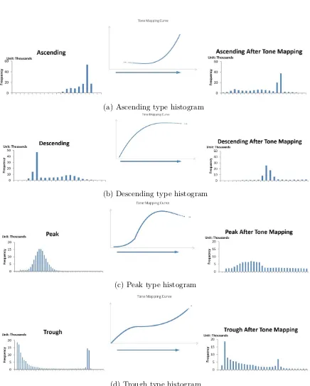
categorize it based on the relative heights of the bins. As illustrated in Figure 2.6,
histogram type can be determined by detecting where the peak is and how many
peaks are there in the histogram.
To customize the mapping curve we use in the fragment shader, we need to first determine what we want to achieve after tone mapping. Our goal is to create one
tone mapping curve optimized in one viewable region that can equalize this region’s
original luminance histogram and stretch it as wide as possible to exploit the limited
available luminance range. For each of the four histogram categories, its final output
can be described as follow:
• Ascending: The whole region needs to be dimmed down and the brighter the pixels are, the more they will be dimmed down.
• Peak: For this type of region, we only need to stretch the histogram reasonably so that its center approximates the center of available luminance range.
• Trough: We want to scale the dim peak to brighten the dim regions and the bright peak down at the same time so that the resulting histogram is equally spread across available luminance LDR.
After we define the resulting histogram, we can have a basic outline of the curve
for each type of histogram. In the early stage of this thesis, we chose Bernstein polynomial because its shape could be directly modified by changing its coefficients.
Because we intended to store tone mapping parameters in another image file and we
could keep up to four parameters as RGBA values in.exr format, we used 3rd order
Bernstein curves which granted us the most controls under the limit of the maximum
number of coefficients we could store. Equation 2.2 is the general form of a 3rd order
Bernstein polynomial:
B3(x) = A(1−x)3+B(3x(1−x)2) +C(3x2(1−x)) +Dx3, (2.2)
A, B, C, D were called Bernstein coefficients. This smooth 3rd polynomial curve was
directly determined by its coefficients in a clear pattern: in its domain, the smooth
curve could be treated as a composition of four segments; from left to right, each segment was associated with A, B, C and D respectively; increasing the value of a
specific coefficient would form a peak in the related segment and decreasing the same
coefficient would result in a trough shape in that segment.
We used linear equation systems to calculate the values of A, B, C and D. The
statistical attributes needed in this approach were minimum, maximum and average
24
cases of Ascending and Descending, statistical attributes could contribute to the following 3 equations:
B3(M in) =M in, (2.3)
B3(M ax) = αM ax, (2.4)
B3(Average) = α
α+ 1(M in+M ax), (2.5)
M in, Average and M axwere statistical attributes of current viewing window,α was
a pre-defined equalization factor which helped to equalize the final histogram in the
range of [0,1.0] after exposure adjustment4. To be more precise, B
3(M ax) would be scaled to approximate to 1.0, and B3(Average) would approximate to the scaled arithmetic mean of minimum and maximum values. Equation 2.5 also determined
whether the calculated Bernstein function was concave or convex. The 4th equation
was different in these two cases. We used the first order derivative of the Bernstein function to constrain the curve’s shape. Equation 2.6 was applied in Ascending
viewing windows and Equation 2.7 was used in Descending viewable regions.
B30(M in) = 0, (2.6)
B30(M ax) = 0, (2.7)
Unlike above cases, Peak and Trough could use the same set of equations. We still used Equation 2.3 and Equation 2.4 to determine the ends of the smooth curve.
Then we divided the pixels into two sub-intervals with average value as the midpoint
4A technique for adjusting the exposure indicated by a photographic exposure meter, in
and traversed the viewing window again to find new average value of each sub-interval,
namelyaverage lef tandaverage right. We conducted two more equations using the
newly computed average values:
B3(Average lef t) = 3α
4α+ 2(M in+Average), (2.8)
B3(Average right) = 3α
2α+ 4(Average+M ax), (2.9)
Using different sets of four equations for different categories, we could create a
linear equation system. Then we used variable elimination that was implemented in
CUDA to solve the system to calculateA, B, C and D.
Based on above algorithm, we could compute a unique set of Bernstein coefficients
for each viewable region and stored the result in an exr file where coefficients are
stored as RGBA values.
Figure 2.6 shows the four base histogram types, the target histograms of each base
type and the curve used to achieve the result. All data comes from viewable regions
in the testing Redwood HDR panorama.
The Bernstein polynomial has advantages such as: computationally efficient, easily parallelizable and flexible to be applied to viewing windows of various luminance
distribution. But there are several fatal limitations that make Bernstein polynomial
inadequate for ToneTexture technique.
• Doesn’t possess second derivative constraint: The constraint on Bern-stein polynomial is not sufficient. The four equations can only put a first
derivative constraint on the curve. The first derivative test locates the functional
26
(a) Ascending type histogram
(b) Descending type histogram
(c) Peak type histogram
(d) Trough type histogram
requires a second derivative test [37]. This lack of constraint leads to weird
behavior of the curve, like the decreasing of the right end in the curve in
Figure 2.6c.
• Lack of simple intuitive controls: Controls should be simple and easy to understand for artists. For 3rd order Bernstein polynomial, the adjustable four
segments have uncontrollable lengths, meaning that the modification made on
one coefficient has different effect on different curves.
• No direct control over dynamic range: Using the Bernstein curve is “all or nothing”. It’s not possible to make a plain linear curve using those controls
because the intersection of the controllable segments can not be changed by adjusting coefficients. There are times where the optimal curve is a plain linear
curve with a slight shoulder to produce softer transition to the overexposed
highlights, and times where the highlights and shadows need to be heavily
compressed.
• No universal solution: While Bernstein polynomial can handle various types of luminance distribution, it requires different solutions for each type. When
the coefficients need to be adjusted after editing, the program has to identify
the current visible region’s luminance distribution type to update the curve of
current window as well as those in windows nearby.
• Lerpable parameters absent: There is no clean blend between different curves in different areas. Lerp is a term for basic operation of linear interpolation
between two values that is commonly used in the field of computer graphics [25].
28
editing on the current visible region, the program should blend the adjustment
into the surrounding windows’ tone mapping parameters. Otherwise, after the
user turns to the window, even if it is one pixel away from the edited one, the modification will not be shown in the new window.
2.2.2 Cubic Spline
Cubic spline, on the other hand, not only possesses all the advantages Bernstein
poly-nomial has, but also triumphs in the aspects where Bernstein polypoly-nomial performs
poorly.
Cubic curves are commonly used in computer graphics because lower order curves
are commonly lacking sufficient flexibility, while curves of higher order are often
considered unnecessarily complex and easily introduce undesired wiggles if handled
without caution. A spline originally means a common drafting tool, a flexible rod, which was used to help draw smooth curves to connect widely spaced points. The
cubic spline curve accomplishes the same task for an interpolation problem. Suppose
we have a data point table containing points represented as (xi, yi) for i= 0,1, . . . , n
for a function y = f(x), where for i ∈ [0, n−1], xi < xi+1. That leaves us n + 1 points andnintervals between them. The cubic spline is a piecewise continuous curve,
passing through each of the points in the table. There is a separate cubic polynomial
for each interval, which is universally defined as:
Si(x) =Ai+Bi(x−xi) +Ci(x−xi)2+Di(x−xi)3 for x∈[xi, xi+1]. (2.10)
Figure 2.7: Cubic spline example for n= 5
points where curve pieces meet are calledknots. Figure 2.7 gives an example of a cubic spline curve wheren = 5. Since there aren intervals and each one of them is fixed by
four coefficients, we require a total of 4n parameters to define the splineS(x). Thus
we need to find 4n independent equations to construct the desired curve.
Here is a summary of the known conditions of the spline:
a) n+ 1 points from the data table: (xi, yi) for i= 0,1, . . . , n.
b) Each spline segment is a third order polynomial curve.
c) At the knots, the spline curve preserves second order parametric continuity.
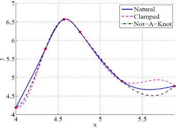
d) Feature of the boundaries at both ends of the interval: Natural Boundary,
Clamped Boundary and Not-A-Knot Boundary.
Condition c) forces the first and second derivatives between adjacent segments to
equal at the knots, which implies that the curve tangents at the join points have not
30
joined spline S(x) is a smooth curve in its domain. The effect of condition d) will be
explained later in this section.
We get 2n equations for each interval from condition a):
Si(xi) =yi (2.11)
Si(xi+1) = yi+1, for i= 0,1, . . . , n−1. (2.12)
Because the spline curve possesses second order parametric continuity, we can
obtain another 2(n−1) more constraints:
Si0(xi+1) = Si0+1(xi+1) (2.13) Si00(xi+1) =Si00+1(xi+1), for i= 0,1, . . . , n−2. (2.14)
where the first and second derivatives of the spline can be easily constructed by
differentiating Equation 2.10:
Si0(x) =Bi+ 2Ci(x−xi) + 3Di(x−xi)2 (2.15)
Si00(x) = 2Ci+ 6Di(x−xi) (2.16)
So far we have 2n+ 2(n−1) = 4n−2 equations. The remaining two equations that we need to completely fix the spline are derived from condition d). Certain
constraints should be put on the derivatives at x0 and xn to limit the boundaries at
the both ends of the domain. There are three traditional options:
S000(x0) = 0
Sn00−1(xn) = 0 (2.17)
• Clamped: The first derivatives at both ends are set to a defined value, namely α and β. This is normally used when there is specific requirement on the tangents at x0 and xn. Then the resulting equations are:
S00(x0) =α
Sn0−1(xn) =β (2.18)
• Not-A-Knot: Instead of specifying any extra conditions at the end points, this constraint forces third order parametric continuity across the second and
penultimate knots of the spline. In this way, cubic polynomials are not changed
when crossing x1 and xn−1, leaving the curve to be more natural and accurate for data interpolation. This can be expressed as:
S0000(x1) = S1000(x1)
Sn000−2(xn−1) = Sn000−1(xn−1) (2.19)
There is no defined way to determine which constraint is better. The choice is made
depending on the application’s expectation on both ends of the curve. Figure 2.8
gives an example of how different boundary conditions affect the ends of the resulting
32
Now that we have 4n linear conditions, next step is to establish the equations
that determine 4n coefficients. The detailed linear equation matrix and solution will
be elaborated in Chapter 3. The one last question for using cubic spline as the tone mapping curve is: what are the points? This question is equivalent to the one
proposed at the beginning of this section: what type of statistical attributes should
be collected?
When S(x) is used to convert an HDR pixel into an LDR pixel, x should be the
original luminance value and y should be the mapped luminance value. To make
full use of the available LDR, yi can be easily determined by dividing the LDR into
equal-length intervals. For normalized LDR, whose range is [0,1.0],yi can be defined
as yi = i×1.0/n for i = 1,2, . . . , n. If we still use minimal, maximal and average
values as we did in Bernstein polynomial method, x0 and xn are the minimal and
maximal luminance in a visible region. xbn/2c is the average that will be mapped to the midpoint in the LDR as ybn/2c, which is 0.5. For n = 2, these three points are all that the data table contains. This limited data table is not sufficiently enough
for cubic spline interpolation and the resulting curve is not accurate nor flexible for
different types of luminance distributions. To refine the curve, we set n= 4, the next
power of 2, so that x1 and x3 are still yet to be retrieved from the captured viewing
34
more data.
This refinement on the curve can keep going for n = 2k where k = 0,1, . . .. The
more data points we use , the finer spline we’ll get. The cost includes the computation to retrieve average luminance values in sub-intervals and the memory needed to store
more coefficients for more segments. Note that by using more average values, there
is no need to identify the region’s distribution type as the spline will automatically
be adjusted under the constraints. In our implementation, we set n = 8 which
is computationally acceptable because there are only log(8) = 3 recursion levels for
retrieving average values and also generates a spline that is flexible and robust enough
to handle different types of visible regions.
When the user wishes to change the coloring emphasis, the simplest way is to mod-ifyxi and re-compute the spline on the fly. For instance, if the user wants to brighten
up the scene, the program should decrease the values of xi for i = 1,2, . . . , n−1
and compute a new spline. As a result, pixels with lower luminance value will be
mapped to higher values by the new spline because yi stays the same. The opposite
modification on the data points will result in a dim-down effect on the visible contents.
However, the interface provided to the user to achieve the desired functionality
should be: organized to save the artist the trouble of changing all data points individually; intuitive as the interface won’t confuse the user to perform intended
coloring modification; easy to use so that even if immersed in a VR environment, the
user should finish the modification task without many errors. Implementation details
CHAPTER 3
IMPLEMENTATIONS
Our work consists of two major components: the ToneTexture generation program usingOpenGLon desktop computer and HDR panorama viewer implemented on both desktop computer andSamsung Note 4 withGear VRHMD. Real-time tone mapping parameter editing is supported on both platforms. The demo viewer on Android
uses Gear VR Framework (GearVRf ), a lightweight, powerful, open source rendering engine with a Java interface for developing mobile VR games and applications for Gear
VR and Google Daydream View. Both implementations support HDR panoramas
up to 16K ×8K in size. Hardware systems include Dell Workstations equipped with NVIDIA Quadro K620 GPU for development and testing, and Samsung Note 4 smartphone with GearVR HMDs. Implementation for both platforms share the same camera configuration so that contents observed by the viewer are constant
and ToneTexture generated for the same panorama can be used in both application versions.
Framebuffer Height 1024
Framebuffer Width 1024
Color Format RGBA (A is for α channel indicating transparency)
FOV 110◦
Multi-sampling 2
36
While Chapter 2 addresses the methods used in this thesis, there are other critical
challenges throughout the development, including implementation details,
perfor-mance improvement and compatibility assurance. The following sections will elabo-rate on these matters.
3.1
Viewing Window Capture
Reading pixels back from the framebuffer inOpenGLis commonly accomplished with the glReadPixels() API. Understanding how this command functions is essential
for achieving good application performance when such read back is incurred.
By default, glReadPixels() reads data from framebuffer objects (FBOs). This
procedure blocks the rendering pipeline until all previous OpenGL commands are executed, and waits until all pixel data are transferred and ready for use before it
returns control to the calling application. It is obvious that this has two negative
performance impacts: forcing a synchronization point between the calling application
and OpenGL, which should always be avoided, and the cost of the data transfer from GPU to central processing unit (CPU) across the bus, which can be fairly expensive depending on how much data is retrieved.
Since the content drawn in the framebuffer has been through rasterisation5, pixel values are stored as single-precision normalized floating point numbers in the range
of [0,1.0]. The size of the FBO equals that of the viewable region. Thus the data for
a single transfer are: 1024×1024×4×4 = 16MB. According to the datasheet for Quadro K620 [9], the raw memory bandwidth on the GPU is 29.0GBps. This is far more than what we need to transfer all the data in an FBO at 60 frames per second
5The task of taking an image described in a vector graphics format (shapes) and converting it
Figure 3.1: Asynchronous glReadPixels() with 2 PBOs
(FPS). But in the development, the capturing program can not achieve such high
FPS. So the bottleneck is not the data transferring but the synchronization where
the GPU must wait for the CPU to complete the calling application’s tasks.
Alternatively,glReadPixels()bound with pixel buffer objects (PBOs) can
sched-ule asynchronous data transfer and returns immediately without any stall. Therefore,
the application can execute other processes like calculating tone mapping parameters
right away while transferring the data by OpenGL at the same time. The other advantage of using PBOs is the fast pixel data transfer from and to GPU though
direct memory access (DMA) without involving CPU cycles. In the conventional
way, the pixel data is loaded into system memory by CPU, whereas using a PBO allows GPU to manage copying data from the framebuffer to a PBO. This means that
OpenGLperforms a DMA transfer operation without wasting CPU cycles. Figure 3.1 illustrates the architecture and processing flow when using two PBOs for asynchronous
reading.
After acquiring pixel data from the framebuffer, the next question is how to
38
visible regions have the same rectangular size, the process of computing tone mapping
parameters can be easily parallelized to achieve high performance. In order for parallel
processing, all captured visible content should be stored as individual HDR images and uploaded to kestrel, a 32-node CPU/GPU cluster from the High Performance
Simulation Laboratory and COEN IT department. Then a program using CUDA and
Message Passing Interface (MPI) would be developed to distribute the computation
among the nodes for shorter execution time. CUDA is a parallel computing platform
and API model created by NVIDIA [10], and MPI is a standardized and portable message-passing system designed to function on a wide variety of parallel computing
architectures [26]. However, there is a fatal drawback in this design. It requires
excessive writing of pixel data to disk to save as individual image files. First, those image files consume colossal physical memory. Ignoring any compression, when using
.exr as the image format, the total raw data takes: 16MB÷2×64800 = 506.25GB (.exr stores pixel data in half precision floating point number per channel). Next,
the function provided by OpenEXR library to write .exr file takes on average one second for each window of designated size, during which time the CPU is completely
blocked without multi-threading. With 64800 visible regions, the total time for image
writing will be an unacceptable 18 hours.
Due to this expensive I/O overhead, we abandoned the parallel processing method, combined the viewport capturing program with cubic spline coefficients calculation
and used the CPU solely to bypass the I/O overhead in file writing. The serialized
implementation takes on an average of 4000 seconds to process one 16K HDR panorama, which is only approximately 6% of the time needed to save viewing
windows in files. This makes the program run at approximately 16 FPS. Given the
CPU is still blocked by calculating the spline during each rendering cycle. Further
improvement can be achieved by implementing a thread pool for multi-threading to
compute the coefficients concurrently. Figure A.1 in Appendix A provides implemen-tation details of the key functions for asynchronous data reading.
When the CPU loads the pixel data from the designated PBO, the first thing to do is to get the luminance values of each individual pixel. Equation 3.1 is a formula
to convert RGB color values to brightness [27]. The formula assigns different weights
to colors in proportion to the human eye’s sensitivity on individual color channels.
In general, humans are more sensitive on green and red components than on blue
channels. If we use the same weight, for example, (R+G+B)/3, then pure red, pure
green and pure blue result in same gray scale level, which conflicts with our perceived
visual experience.
Luminance= 0.299∗R+ 0.587∗G+ 0.114∗B (3.1)
After converting RGB values to luminance, the brightness information of a visible
region can be now stored in a one-dimensional array. To find the data points for
constructing tone mapping spline, we have to traverse the array multiple times to
calculate the averages of the entire data domain and the sub-intervals separated by upper level average values. Since all n data points are monotone increasing in xi for
i ∈ 0,1, . . . , n, one way to efficiently calculate the average values in sub-intervals is to sort the array before the calculation function is called. Another benefit for using
sorted data is that calculation in the next step can be solved in a divide-and-conquer
manner without worrying about different lengths of the sub-intervals. Suppose the
40
Algorithm 1 Finding averages values in Luminance[m] as xi forn data points function findDataPoint(x, Luminance, lef t, right)
sum←0, startIdx←0 mid←(lef t+right)/2
while Luminance[startIdx]< x[lef t] do . find the starting index startIdx←startIdx+ 1
end while
endIdx←startIdx
while Luminance[endIdx]< x[right] do sum←Luminance[endIdx]
endIdx←endIdx+ 1
end while
x[mid]←sum/(endIdx−startIdx)
if mid−lef t >1 then
f indDataP oint(x, Luminance, lef t, mid) f indDataP oint(x, Luminance, mid, right)
end if end function
procedure Find Data Points(Luminance, m, n)
mergeSort(Luminance,0, m) .sort the Luminance array first x[0]←Luminance[0], x[n]←Luminance[m]
f indDataP oint(x, Luminance,0, n)
be efficiently sorted using merge-sort whose average and worst-case performance is O(mlog(m)) [19]. Another reason for choosing merge sort over quicksort is that unlike some efficient implementations of quicksort, merge sort is a stable sort, even though it does not sort in place [8]. But since memory is not our concern, this sorting
method becomes optimal for the task. The runtime for finding the average of raw
HDR luminance is O(m) because traversal through the entire array at least once is
required. In the next level of recursion, the sorted data are divided into two halves
using the newly-found average value as midpoint and the size of each sub-interval
can be noted as m1, m2 respectively with m =m1+m2. The total running time at the second recursion level is thereforeO(m1) +O(m2) = O(m). Thus the recurrence
T(m) = T(m1) +T(m2) +O(m) follows from the definition of the algorithm. Since there will be log(n) recursion levels, the complexity to retrieve all average values
is mlog(n). In our implementation, n = 8, meaning that we can treat log(n) as
constant. As a conclusion, the runtime for finding needed data points should be:
O(mlog(m)) +O(m) = O(mlog(m)). This procedure is concluded in Algorithm 1.
3.2
Cubic Spline Coefficients
After retrieving average values from a captured viewing window, we need to calculate
for an optimized cubic spline using the data point table. In Subsection 2.2.2, the
mathematical representation of a cubic spline is given as Equation 2.10:
Si(x) =Ai+Bi(x−xi) +Ci(x−xi)2+Di(x−xi)3 for x∈[xi, xi+1]. (2.10 revisited)
We also specify four constraints to construct this piecewise cubic spline with
42
for the functiony=S(x), in which for every i∈[0, n−1],xi < xi+1. The constraints are summarized in the following five equations:
• Continuity in data points:
Si(xi) =yi (2.11 revisited)
Si(xi+1) = yi+1, for i= 0,1, . . . , n−1. (2.12 revisited)
• Continuity in derivatives:
Si0(xi+1) = Si0+1(xi+1) (2.13 revisited) Si00(xi+1) =Si00+1(xi+1), for i= 0,1, . . . , n−2. (2.14 revisited)
• Natural boundary:
S000(x0) = 0
Sn00−1(xn) = 0 (2.17 revisited)
from these constraints, 4n linear equations are derived to determine 4n coefficients.
This section will give details on establishing a linear equation matrix and applying
the Tridiagonal Matrix Algorithm to solve the linear system.
Define the points’ step length in X axis as: hi = xi+1 − xi and start from
Equation 2.10, then we can get:
a. Derived from Equation 2.11:
b. Substitutexi+1−xi with hi in Equation 2.12:
Ai+hiBi+hi2Ci+hi3Di =yi+1 (3.3)
c. From Equation 2.13:
Si0(xi+1) =Bi+ 2Cihi+ 3Dihi2 Si0+1(xi+1) =Bi+1
=
⇒Bi+ 2Cihi+ 3Dihi2 =Bi+1 (3.4)
d. Based on Equation 2.14:
2Ci+ 6Dihi = 2Ci+1 (3.5)
Define the second order derivative asmi =Si00(xi) = 2Ci. Then from Equation 3.5,
Di can be represented as:
Di =
mi+1−mi
6 (3.6)
The only coefficient left is Bi. Substitute Ai, Ci and Di with mi in Equation 3.3,
we can get:
Bi =
yi+1−yi hi
− mi+1+ 2mi
6 hi (3.7)
Since all the coefficients are either known values (yi and hi) or represented by mi,
we only need to establish one equation for the linear matrix. Substitute all coefficients
44
yi+1−yi hi
− mi+1+ 2mi
6 hi +mihi+
mi+1−mi
2 hi =
yi+2−yi+1 hi+1
− mi+2+ 2mi+1
6 hi+1 =
⇒himi+ 2(hi+hi+1)mi+1+hi+1mi+2 = 6(
yi+2−yi+1 hi+1
−yi+1−yi hi
) (3.8)
Note that Equation 3.8 is only for i ∈ [0, n−2], which can only contribute to n−1 rows in the linear matrix while there are n+ 1 rows in total for mi from m0 to mn. The remaining two equations are derived from Natural Boundary constraint
(Equation 2.17):
m0 =mn = 0 (3.9)
Hence, the matrix can be established as:
1 0 0 0 0 . . . 0
h0 2(h0+h1) h1 0 0 . . . 0
0 h1 2(h1+h2) h2 0 . . . 0
0 0 h2 2(h2+h3) h3 . . . 0
..
. ... . .. . .. . .. ...
0 . . . 0 0 hn−2 2(hn−2+hn−1) hn−1
0 . . . 0 0 0 0 1
m0 m1 m2 m3 .. .
mn−1
mn = 6 0
y2−y1
h1 −
y1−y0
h0
y3−y2
h2 −
y2−y1
h1
y4−y3
h3 −
y3−y2
h2
.. .
yn−yn−1
hn−1 −
yn−1−yn−2
hn−2
0 (3.10)
This linear equation system is a tridiagonal system since the matrix on the left is a tridiagonal matrix. In linear algebra, a tridiagonal matrix is a specific type of
square matrix that has nonzero elements only on the main diagonal and along the
subdiagonal6 and superdiagonal7. For such systems, the solution can be obtained in O(n) operations instead of O(n3) required by conventional Gaussian elimination [1]. The efficient solution is named Tridiagonal Matrix Algorithm, also known as the
6Comprised by elements directly under the main diagonal.
Thomas Algorithm (named after Llewellyn Thomas). It is a simplified form of Gaussian elimination that consists of two phases: a forward elimination to convert
the matrix into an upper triangular matrix and a backward substitution to produce the solution. Detailed explanation on the algorithm can be found in Appendix B
After solving the equation system, coefficients can be obtained using Equation
(3.2), (3.6) and (3.7) while Ci = m2i. These coefficients are stored in a texture
file which functions as a look-up table for tone mapping. Notably, since the most
computationally expensive operation is the one retrieving data points and calculating
average values in different intervals, xi is also saved for real time editing. After
manipulating the data points, we can control the spline by re-computing coefficients
to interpolate new data. Even though the spline curve can be affected by all data points individually, it is not an optimal interface design to grant user direct control on
every point, especially when the user is isolated and immersed in the VR environment.
This calls for an interface that groups modification on knots from different luminance
regions while providing easy and intuitive control on the mapping curve.
3.3
Editing Interface
Even though HDR imagery isn’t the mainstream in digital imagery, it has been a research topic for decades. Tone mapping, however, has been studied even longer by
traditional film photographers instead of computer scientists. In film photography,
contrast is one of the most significant characteristics of an image [36]. As a display
medium, films only have a limited exposure range in which they can produce contrast.
If areas of a film receive exposure either below or above the useful exposure range,
46
for converting differences in exposure (subject contrast) into film contrast (differences
in density). The “exposure-to-film-density” curve, referred to as Filmic curve in
computer graphics, functions equivalently as a tone mapping curve in HDR-to-LDR conversion. Since film photographers have researched the curve and developed an
intuitive customization system for different coloring emphasis, the editing interface
for ToneTexture adapts from the Filmic curve adjustment to achieve simple and intuitive control while producing aesthetic result.
Figure 3.2: Components in a Filmic curve, example took from John Hable’s blog
As shown in Figure 3.2, similar to piecewise cubic spline, a Filmic curve is made
of three distinct regions with different mapping characteristics. The part of the curve
associated with low luminance is referred to as the toe, which corresponds to the
dim portions of an LDR image. The shoulder is responsible for transfer contrast in
areas that receive relatively high exposures to the maximal luminance that is mapped
(a) Three types of toes (b) From up to bottom: concave down-wards, linear and concave upwards
Figure 3.3: (a). Three types of toe. (b). Effect on dark luminance of the same color by different toes
changing the content contrast. This part is of least concern since it has minimal impact on the resulting image.
Different toes result in different coloring effects on the dark end. Toes can be
categorized by its shape: concave downwards, linear and concave upwards, as shown
in Figure 3.3a. A concave down curve is a curve that for every point on the curve,
the tangent line to the curve at that point lies above the graph in the vicinity of the
point and a concave up curve is defined in an opposite situation where the tangent
line lies below. A concave downwards toe brings up the low value. This is reflected in the desaturated blacks in the dark regions. On the contrary, a concave upwards toe
brings down high values, leading to more saturation in the blacks. This is illustrated
in Figure 3.3b. There can be a bi-directional control on our spline to adjust the toe
from concave downwards to concave upwards, using arrow key buttons or joysticks