High voltage earthing system testing - an investigation into the effects of test lead coupling on test results

University of Southern Queensland

Faculty of Engineering and Surveying

High Voltage Earthing System Testing :–

An Investigation into The Effects of Test Lead Coupling on

Test Results

A dissertation submitted by

Cameron Brandis

In fulfilment of the requirements of

Courses ENG4111 and 4112, Research Project

Towards the degree of:

Bachelor of Engineering (Electrical and Electronic)

Abstract

High Voltage Earthing System testing is the focus of this research project, in particular the effects

of test lead coupling when conducting soil resitivity tests. Many of the tests conducted to verify the

correct and efficient design of an Earthing system, are carried out using and AC signal of specified

frequency, with very low level readings of voltage and current recorded by a test set or technician.

With measured signals being very low amplitude (often in the milli-volt and milli-ampere range, for

example) the effects of test lead coupling, can reasonably be expected to have a significant effect on

the results obtained.

The intent of this research project is to attempt to quantify such effects and to deduce a

mathematical relationship to predict or quantify coupling effects. The aim is to allow for improved

Certification

I certify that the ideas, designs and experimental work, results, analyses and conclusions set out in

this dissertation are entirely my own effort, except where otherwise indicated and acknowledged.

I further certify that the work is original and has not been previously submitted for assessment in

any other course or institution, except where specifically stated.

Cameron Brandis

Student Number: 0050008387

_________________________

(Signature)

__________________________

Acknowledgements

For their assistance, advice and expertise, I wish to thank:

•

Mr. Andrew Hill, Hydro Tasmania Consulting. For his expertise and advice on all aspects of

High Voltage Earthing systems and the testing of such systems.

•

Downer EDI Engineering. For their time and assistance in conducting tests, use of

equipment, technical guidance, and good humour in the completion of this project.

•

My wife, Shanan and son Michael, for their understanding and support in completing this

Degree program over the last seven years on a part time basis.

Cameron Brandis

University of Southern Queensland

Table of Contents

1.1 Introduction... 1

2.

Literature Review... 3

2.1 Literature Selection... 3

2.1.1 Relevant Standards and Codes... 3

2.1.2 Text Books and Literature Relevant to Electro Magnetics... 4

2.1.3 Technical References Relevant to Test Equipment Used ... 5

2.2 Project Justification... 6

2.2.1 Improvement in Design and Verification ... 6

2.2.2 Cost Savings ... 6

2.2.3 Improved Safety and Stability ... 6

3.

Methodology... 8

3.1 Project Methodology... 8

3.1.1 Technical Research ... 8

3.1.2 Conducting of Tests... 8

3.1.3 Analysis of the Results... 9

4.

High Voltage Earthing Systems ... 10

4.1 The High Voltage Substation Earthing System ... 10

4.1.1 Function and Design of an Earthing system ... 10

4.1.2 Earthing System Types ... 12

5.

Earthing System Testing... 17

5.1 Earth Resistivity Testing... 17

5.1.1 The Wenner Array Method... 18

5.1.2 The Schlumberger Array Method... 20

5.1.3 The Driven Rod (3 Pin) Method... 21

6.3.2 Resistivity Curves Calculated From Measured Resistance – Caboolture Site... 31

6.3.3 Resistivity Curves Calculated From Measured Resistance – Pittsworth Site ... 32

6.3.4 Resistivity Curves as Calculated From Measured Resistance Vs Measured Voltage and Current: Megger DET2/2 Instrument – Caboolture Site... 33

6.3.5 Resistivity Curves as Calculated From Measured Resistance Vs Measured Voltage and Current: Fluke 1625 Instrument – Caboolture Site... 34

6.3.6 Resistivity Curves as Calculated From Measured Resistance Vs Measured Voltage and Current: Megger DET2/2 Instrument – Pittsworth Site ... 35

6.3.7 Resistivity Curves as Calculated From Measured Resistance Vs Measured Voltage and Current: Fluke 1625 Instrument – Pittsworth Site ... 36

6.4 Discussion of Initial (Stage 1) Test Results... 37

6.4.1 Test Lead Coupling and the Resistance Indicated by the Test Instrument... 37

6.4.2 Test Lead Coupling and the Measured Voltage and Current Signals... 38

6.5 Further Testing Based on Results of Initial Tests. (Stage 2 Tests)... 39

6.5.1 Results Obtained from Stage 2 Tests... 39

6.6 Discussion of Stage 2 Test Results ... 41

6.7 Further Testing Based on Results of Stage 1 and 2 Tests. (Stage 3 Tests)... 45

6.7.1 Results of Stage 3 Tests ... 46

6.8 Discussion of Stage 3 Test Results ... 47

7.

Theoretical Effects... 50

7.1 Calculation of Circuit Inductive and Capacitive Effects - Parallel Test Lead Layout.. 51

7.1.1 Calculation of Circuit Inductance Effects ... 51

7.1.2 Calculation of Circuit Capacitance Effects... 53

7.2 Calculation of Equivalent Current Injection Circuit and Injected Current Waveform

Shape... 56

7.3 Sample Results Obtained From MATLAB Program... 60

8.

Conclusions ... 62

8.1 Achievement of Project Objectives ... 62

8.2 Recommendations... 62

8.3 Further Work and Potential Future Research Projects... 63

8.4 Conclusion ... 63

List of Appendices

Appendix A - Project Specification 71

Appendix B - Risk Assessment and Workplace Health and Safety 74

Appendix C – Schedule Of Tests 77

Appendix D – Multimeter and Clamp Meter Accuracy Specifications 78

Appendix E – Resistivity Results for Caboolture and Pittsworth Sites – Stage 1 Tests 81

List of Figures

Figure 1: Example of a High Voltage Substation Earthing Grid...11

Figure 2: TT Earthing System. ...14

Figure 3: TN Earthing System.. ...15

Figure 4: IT Earthing System. . ...15

Figure 5: Resistivity. Conductor of 1m cross sectional area, and 1m length ...18

Figure 6: Wenner Array. Probe layout and injected and measured signals...20

Figure 7: Schlumberger Array. Probe layout and injected and measured signals ...21

Figure 8: 3 Pin Array. Probe layout and injected and measured signals ...22

Figure 9: Test Leads at 90°...24

Figure 10: Test Leads in Parallel (0°)...24

Figure 11: Test Leads in Parallel (180°)...25

Figure 12: Parallel Test Lead Configuration. ...25

Figure 13: Example Square Wave. ...26

Figure 14: Resistivity Curves. DET2/2 - Caboolture Site. ...31

Figure 15: Resistivity Curves. Fluke 1625 - Caboolture Site...31

Figure 16: Resistivity Curves. DET2/2 - Pittsworth Site. ...32

Figure 17: Resistivity Curves. Fluke 1625 - Pittsworth Site. ...32

Figure 18: Resistivity Curves. Megger DET2/2 - Caboolture Site...33

Figure 19: Resistivity Curves. Fluke 1625 - Caboolture Site...34

Figure 20: Resistivity Curves. Megger DET2/2 - Pittsworth Site. ...35

Figure 21: Resistivity Curves. Fluke 1625 - Pittsworth Site. ...36

Figure 22: Voltage and Current Waveforms, 90° Test lead Orientation: ...40

Figure 23: Voltage and Current Waveforms, Parallel 0° Test lead Orientation:...40

Figure 24: Voltage and Current Waveforms, Parallel 180° Test lead Orientation....41

Figure 25: Typical Voltage Waveform (Channel A)...42

Figure 26: Typical Current Waveform (Channel B)...42

Figure 27: Typical Inductive Voltage and Current Waveforms ...44

Figure 28: Voltage and Current Waveforms for probe spacing of 150m ...46

Figure 30:

2 Wire transmission line and magnetic field ...51

Figure 31:

2 Wire transmission line ...53

Figure 32:

R-L Circuit current waveform...58

Figure 33:

Program flowchart for calculation of R-L circuit current waveform..59

Background

1.1

Introduction

Modern electricity supply systems are complex integrated systems which allow the transmittal of

large quantities of electrical energy over great distances. From the point of generation, electricity is

transmitted through an interconnected network of lines and substations, to a multitude of different

locations, eventually arriving at the point of final usage, by the customer. Such a large and complex

network can be thought of as many smaller sub systems operating in unison to deliver a safe,

economic and reliable supply of electricity to the consumer.

One such system that forms an integral part of the safe and efficient operation of any electricity

system, is the High Voltage Earthing System, specifically the earthing systems associated with high

voltage substations. Earthing systems are generally applicable, to all stages of electrical power

systems including generation, transmission, distribution and utilisation. This dissertation is

primarily concerned with high voltage earthing systems, as would be found in any high voltage

substation, and in particular the testing and design verification of such earthing systems.

High Voltage Substation earthing systems, form one component within a high voltage electrical

system, and perform several functions. Typical functions of a High Voltage Earthing System

include the safety of plant and personnel, equipment protection and correct electrical system

operation. With such functions as these, it becomes immediately evident that an Earthing system

must be adequately designed and tested, prior to being placed in service, to ensure fulfilment of

such requirements.

In a General sense, any installation must undergo some form of testing during each of the stages of the

system’s intended life, to ensure correct and proper operation. Substation earthing is no different, and testing

is required in several stages of the design, installation and operation phases of an earthing system. In the

context of this research project, the stages of importance may be considered as the conceptual (design) phase,

the post construction-pre-commissioning phase, and the maintenance phases of an installed system.

During the design phase, accurate data is required of the soil resistivity, which is a term used to describe the

conductive properties of the soil. The soil resistivity is required to determine the Earthing system design,

including the spacing, size and number of conductors installed to form the earthing system. Using modelling

techniques, the soil resistivity also can be used to determine how the theoretical earthing system may operate

In the post construction, pre-commissioning phase, tests are completed to assess the performance of the

earthing system, prior to it being placed in service. Tests conducted at this stage will be used to verify the

theoretical calculations used in the design of the earthing system, and also to identify any areas in need of

improvement, prior to commissioning of the system.

Maintenance testing can be considered as a verification of the integrity and correct operation of the earthing

system, once it has been in service for a given period of time. Deterioration of the earthing system due to

corrosion, for example, can lead to significant problems associated with safety and a reduction in the

performance of the earthing system, in the case of a fault on the electrical network.

Earthing testing is the focus of this research project, in particular the effects of test lead “self coupling” when

conducting soil resistivity tests. Self coupling in this context, refers to the electrical test signals, creating

interference between the test leads used to conduct the test. This interference creates an error in the results

obtained, and therefore reduces the quality of the results obtained.

Many earth resistivity tests conducted for an earthing system are carried out using an alternating current

(AC) or alternating direct current (DC) signal of specified frequency, with very low level readings of voltage

and/or current measured by the test set or technician. With measured signals being very low amplitude (in

many cases in the millivolt or milliamp range) the effects of test lead coupling, can reasonably be expected to

have a significant effect on the results obtained. The intent of this research project is to investigate and

attempt to quantify such effects and to deduce a mathematical relationship to predict or quantify self

coupling effects. The aim is to allow for improved test accuracy and hence improve the quality of the results,

2.

Literature Review

2.1

Literature Selection

The range of literature and information available relevant to substation earthing testing and the effects of

coupling have been classified into three areas.

• Standards and codes relevant to electrical earthing

• Text books and literature relevant to Electro Magnetics and Inductive and Capacitive Coupling • Technical references relevant to test equipment used.

2.1.1

Relevant Standards and Codes

There are several standards relevant to earthing of electrical apparatus, and low frequency induction. The

known standards, which will be utilised for this research project are:

• IEEE 80: 2006 Guide for Safety in AC Substation Grounding • ENA EG1: 2006 Substation Earthing Guide

• SAA HB 102: 1997 - Coordination of Power and Telecommunications – Low Frequency Induction • The Australian and New Zealand standard AS/NZS 4360:1999 together with Downer EDI

Engineering’s Risk Assessment procedures will be used as a reference to establish and implement

the risk management process.

Several notable excerpts from the above documents have been included due to their relevance to this research

project, as follows.

Chapter 5, ENA EG1: When conducting resistivity tests, measurements at larger spacings often present

considerable problems such as inductive coupling, insufficient resolution on test set and physical barriers.

Chapter 5, ENA EG1: States practical testing recommendations, for soil resistivity tests. Of relevance to this

discussion, is the first point in the list on page 29:

• Eliminate mutual coupling or interference due to leads parallel to power lines. Cable reels with parallel axes for current injection and voltage measurements, and small cable separation for large

Chapter 11, ENA EG1: Mention is made of the need to exercise caution to ensure that conductive and

inductive interference components are taken into account when conducting Impedance and Step, Touch and

Transfer voltage measurements.

Chapter 11, ENA EG1: Calculation of system impedance is made using the given equation (Eqn 11-1) and

the assumption that measurements are not influenced by mutual coupling or other interference. There appears

to be no means by which to calculate or account for such interference, other than the testing guidelines to

minimise coupling effects as stated in section 11.1

Perhaps the most notable reference is made in section 11.2.3 of the ESAA EG1. It states:

“For a complex electrode, such as an earthing system of a substation, the earth resistance is very low. Many

instruments cannot measure low resistances and the great majority of them do not account for the reactive

part. In addition to the required instrument capabilities, testing configuration and analytical calculations are

required to handle errors due to power frequency standing voltages and injection current induced voltage

errors.”

All of these quotes outlined above, add further weight to the need and hence purpose of this project to

investigate the effects of test lead coupling. It should be noted that while general recommendations exist to

avoid test lead coupling, there appears to be little or no specific information on the required separation of test

leads, lead layout patterns, or the means of calculating interference.

2.1.2

Text Books and Literature Relevant to Electro Magnetics

There is a large amount of literature and text books available relevant to electromagnetics, however for the

sake of simplicity and ease of reference, several sources have been selected, each of which is detailed below.

Grainger and Stevenson: Chapter 4 details the means to calculate flux linkages between

transmission lines of varying configuration. The portion of greatest interest is likely to be section

4.6, I.e. The inductance of a single phase two wire line (as is the case during earthing testing).

SAA HB 102: Section 2 details the method of calculating induced voltages in parallel lines, which

is again of relevance to the interference we expect to encounter.

2.1.3

Technical References Relevant to Test Equipment Used

The test equipment selected for use in this project was originally intended to be limited to two

pieces of test equipment, each of different purpose and function. These items of were initially

proposed as 1) an earth resistivity test set, and 2) a current injection test set. During the completion

of this research project, the equipment selection was revised, based on the realisation that the scope

of research required for two different test functions, was unachievable in the time allocated, and

resource availability for completion of the project. The equipment selection hence became limited

to two items of similar function, capable of testing Earth Resistivity, which has become the main

test function under analysis in this project. The equipment selection and relevant documentation has

thus been limited to:

• Fluke 1625 GEO Earth Ground Tester, User Manual, Fluke Corporation, 2006

•

Relevant sections of these instruction manuals have not been included, as there are a large number

relevant sections, too numerous to be adequately included here. These documents primarily deal

with the carrying out of tests and the recording of results, and hence contain large amounts of

2.2

Project Justification

Substation earthing testing is by no means a new field as there is a large amount of relevant literature

available, however, to date there appears to be little, or no analysis undertaken on the effect of errors

introduced, through electromagnetic interference due to self coupling effects. Currently tests are conducted

and the results obtained are assumed to be correct, with little consideration given to possible errors

introduced by the test leads themselves. Errors introduced can have significant effects on the overall earthing

system in the design, installation and operational stages of the substation in question. Such errors, duly

identified and allowed for, yield following consequences.

2.2.1

Improvement in Design and Verification

The allowance for, or correction of, errors introduced will inherently mean a more accurate and effective

earthing system is able to be designed and installed, to perform all of the required functions of such an

earthing system.

2.2.2

Cost Savings

The implementation of an improved earthing system by design, may lead to reduced equipment and

installation costs. An accurately designed earthing system may require considerably less earthing conductors

and electrodes to be installed, leading to considerable savings in material, labour and installation costs.

Correct initial design also alleviates the need for alteration or re-work of poorly designed earthing

installations.

2.2.3

Improved Safety and Stability

constant voltage and frequency at all times. In practical terms this means that both voltage and frequency

must be held within close tolerances so that the consumer's equipment may operate satisfactorily. For

example, a drop in voltage of 10-15% or a reduction of the system frequency of as little as 5-10 % may lead

to stalling of some motor loads on the system. Effective earthing systems allow for improved fault clearing

3.

Methodology

3.1

Project Methodology

To effectively investigate the effects of test lead coupling, the methodology to employed, can be broken into

three broad categories, Technical research, conducting of the tests and analysis of the results.

3.1.1

Technical Research

Before analysing the effects of test lead coupling, the process of carrying out earthing testing had to be

understood. Information was gathered on the complete range of tests as well as the processes involved and

the reasons for conducting such tests. Information on the signals injected and measured, the calculations

applicable and the analysis required are all relevant to help determine the signals and tests which may be

affected by coupling effects. From this research, one particular test was selected to be researched further,

based on the test characteristics and the likelihood to suffer from interference and coupling. Based on the

technical research completed, the test process to be analysed further is:

• Soil Resistivity Testing

Soil Resistivity has been selected based on the criteria that the signals to be injected and measured are of low

level and are likely to be significantly altered by the effects of inductive coupling. Expected values of

injected current are in the milliamp range, and measured voltages, are similarly in the millivolt range.

Relevant sources of information for the methods used to carry out soil resistivity testing have been listed in

the “Literature Review” section. The specifics of the test instruments and test process is outlined further in

section 4.

3.1.2

Conducting of Tests

3.1.3

Analysis of the Results

Once the schedule of tests was complete, analysis of the results was conducted to try and determine the

effects and situations where coupling is present. This analysis had the broad aims of:

• Determining the level of interference due to coupling, based on data obtained • Determining situations and configurations where coupling is likely to be present

4.

High Voltage Earthing Systems

4.1

The High Voltage Substation Earthing System

4.1.1

Function and Design of an Earthing system

A high voltage earthing system is generally comprised of two functions, namely the provision of a low

impedance connection to the general mass of earth, and the connection of the electrical system, to this low

impedance connection to earth.

With regard to the provision of a low impedance connection to the general mass of earth, this may be

achieved by a number of means, generally involving the burial of a number of conductors and/or electrodes,

in some form of predetermined arrangement, at a specified depth and spacing. This series of conductors and

electrodes is commonly referred to as an “earth grid”. The earth grid design including the number of

conductors, electrodes, spacing and depth of burial, is determined by the site properties and the intended use

for the site.

Examples of the factors to be taken into consideration, when designing an earth grid, include:

• The required conductor spacing and depth - determined by a number of factors such as the prospective fault current level of the site, conductive properties of the soil, soil profile levels, etc

• The conductor size, and conductor material – determined by factors such as required fault current carrying capacity, required mechanical strength, corrosive properties of the soil, etc.

There are many different materials suitable for use as a conductor or electrode in an earth grid. Examples of

Examples of typical earth grid arrangements include:

• Strips of conductor or bare cables laid in mesh pattern to form a Horizontal mesh.

• A series of rods connected with suitable cabling

• A series of rods drilled deep into the earth and connected via cabling back to a central connection point

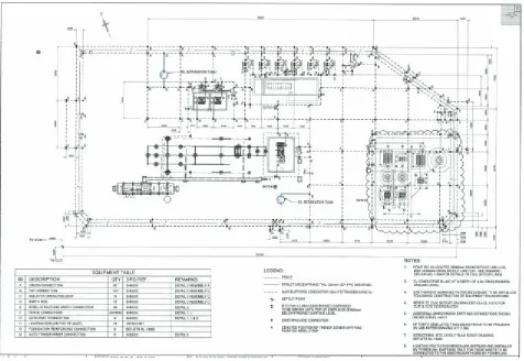
Figure 1 shows an example of a schematic of a typical earthing grid, designed for a High Voltage substation

Figure 1: Example of a High Voltage Substation Earthing Grid (Reproduced with permission of Downer EDI Engineering)

As detailed in section 2, The Electricity Supply Association of Australia (ESAA) and Institute for Electrical

and Electronic Engineers have each released standards applicable to High Voltage Substation Earthing

systems. These documents are the Substation earthing Guide (ENA EG1 (2006)) and The IEEE Guide for

Safety in AC Substation Grounding (IEEE 80 (2000)). These documents detail the following, as typical

Safety:

• To ensure that metallic structures and equipment within a substation are maintained at the same potential.

• To discharge any induced potentials or static build up that may be present.

• To ensure that hazardous step and touch potentials do not exist during a fault event, either at system frequency or due to transient disturbance

• The design criteria are maintained over the design life of the installation despite additions or modifications.

Equipment Protection:

• To limit the level of transient voltages present on equipment by safely providing a low impedance path for lightning discharges, switching surges, fault currents and other system

disturbances. Without adequate earthing system protection, equipment damage may become

extensive and can include insulation breakdown, thermal or mechanical damage, fire or

electrically generated explosions.

• To limit the level of interference and or damage caused to sensitive electronic protection and control devices as a result of such transient voltages being present on the power system.

Correct Electrical System Operation:

• To ensure the correct and timely operation of protective devices in the case of abnormal system conditions.

• To limit the overall disturbance to the power system as a result of a fault event

As can be clearly seen by these reasons, any high voltage electrical substation must therefore have an

connections based on the connection arrangement in use. There exists several different means of connection

of electrical equipment to an Earth Grid, and for a typical system, IEC 60364:2001 defines the types of

earthing systems by a lettering system, as follows:

First Letter – The relationship of the power system to earth

T: Direct connection of one point to earth

I: All live parts isolated form earth, one part connected through an impedance

Second Letter – The relationship of the exposed conductive parts of the installation to earth

T: Direct electrical connection of exposed conductive parts to earth, independently of the

earthing of any part of the power system

N: Direct electrical connection of exposed conductive parts to the earthed point of the power

system (the neutral in AC systems)

Subsequent Letters (if any) – Arrangement of neutral and protective conductors

S: Protective function provided by a conductor separate from the neutral or the earthed line

(phase) conductor

C: Neutral and protective functions provided in a single conductor

Several examples of commonly used earthing systems within Australia include:

Direct Earthing: Protective earths are connected by an electrode or series of electrodes, to the general

mass of earth. Using the letter designations detailed above, this system is called the TT earthing system and

relies on a low impedance connection to the mass of earth to provide a low impedance path through which

any earth fault current will flow. If the connection to the general mass of earth is of high impedance, then the

resulting earth fault current will become limited, and may lead to a fault remaining undetected or uncleared

as well as damage to equipment and dangerous voltage potentials. This system is widely used in High

voltage electrical substations, where transmission voltages are used (33kV and above)

Multiple Earthed Neutral (MEN) System: Protective earths are connected to the system neutral

conductor at the source and at multiple points along the system. This system is designated the TN system of

earthing and operates on the presence of multiple connections of the neutral conductor to the general mass of

earth. By connecting the neutral at many locations the overall impedance of the connection to earth becomes

very low, hence promoting large earth fault currents, which are easily detected. Because this system uses a 4

method of connection (i.e no neutral conductor). Figure 3 depicts a typical MEN system. The MEN system is

the predominant method in use for low voltage electrical systems (230/400VAC) within Australia.

Impedance Earthed System: The installation is either isolated from earth, or connected to Earth through

an impedance to limit the fault current. This system is designated the IT system, where the magnitude of

earth fault current is limited by the impedance of the return path. This system is frequently used in High

voltage substations using distribution voltages (11kV and 22kV), to limit the flow of earth fault current to a

reasonable (and less damaging level). A diagram of an Impedance earthed system is shown in figure 4.

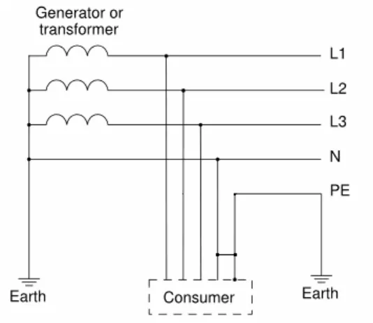
Figure 3: TN Earthing System. Note direct connection of supply source to Earth, as well as neutral conductor connection to earth at source and consumer terminals.

Figure 4: IT Earthing System. Note connection of supply source to Earth via an impedance, Z.

From the systems discussed, a High Voltage substation earthing system can thus be considered as either a TT

or IT system, where the high voltage system is earthed directly (TT System) or via an impedance (IT system)

The TT system, is widely used in transmission type substations (i.e EHV substations with voltages of 66kV

part of the fault circuit will be directly connected to earth and hence ensure rapid isolation of the faulted

plant or equipment. Rapid isolation of faults in the EHV network is critical to the stability of a power system,

as these lines form the main points of connection between power stations and distribution networks. (source:

Network Protection and Automation Guide, Alstom, 2002)

The IT system is more widely used in major substations operating at a lower voltage level, such as would be

found in distribution type zone substations (11kV or 33kV for example). Reduced voltage levels inherently

lead to increased current levels, in order to deliver the same amount of power to the required load or system.

For a fault close to the substation, destructive earth fault currents may hence occur, or high earth potential

rise on the main earth grid. To limit the fault current an impedance (commonly a resistance or reactance) is

chosen and installed in the earth return path to the main transformer at the substation. (source: Network

5.

Earthing System Testing

High Voltage Earthing system testing is divided into two stages, namely, tests to be completed prior to

installation, and tests to be completed after installation and prior to commissioning. Maintenance testing can

be argued to be a third stage, however the tests conducted as part of routine maintenance are a replication of

some or all of the tests completed in the post installation – pre commissioning phase.

The tests conducted prior to installation are primarily concerned with obtaining information about the site

geology and soil properties, in order to accurately design the earthing system for the proposed site. Tests

conducted in this phase are primarily concerned with the soil Resistivity. Tests conducted in the post

installation – pre commissioning phase include, Earthing system impedance, Earth grid Potential rise,

Current Distribution tests, and Step and Touch Voltage tests. As this research project is based primarily

around the effects of coupling during Resistivity tests, the following discussion will focus around Resistivity

testing only.

5.1

Earth Resistivity Testing

The Resistivity of a material is defined as

L

RA

=

ρ

where

R = resistance of the material,

A = cross-sectional area through which current flows and

L = length of the material.

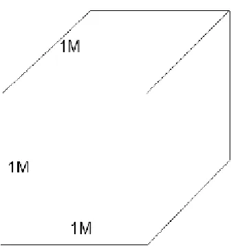
Resistivity is therefore a measure of the electrical resistance of a conductor (in this case the soil) of 1 unit

cross-sectional area and 1 unit length. Think of a 1m x 1m x 1m cube of soil with a metallic plate fixed to

each end. The resistivity in this case is the resistance between the two plates, and hence is measured in ohm

metres (Ωm). Resistivity is a characteristic property of the soil, and is useful in comparing various soil types, based on their ability to conduct electrical current. High soil Resistivity designates a poor conducting soil,

Figure 5: Resistivity. Conductor of 1m cross sectional area, and 1m length

ENA EG1, 2006 states there are three common test methods, for conducting soil resistivity tests. These three

methods are:

• Wenner Array Method

• Schlumberger Array Method

• Driven Rod Method

5.1.1

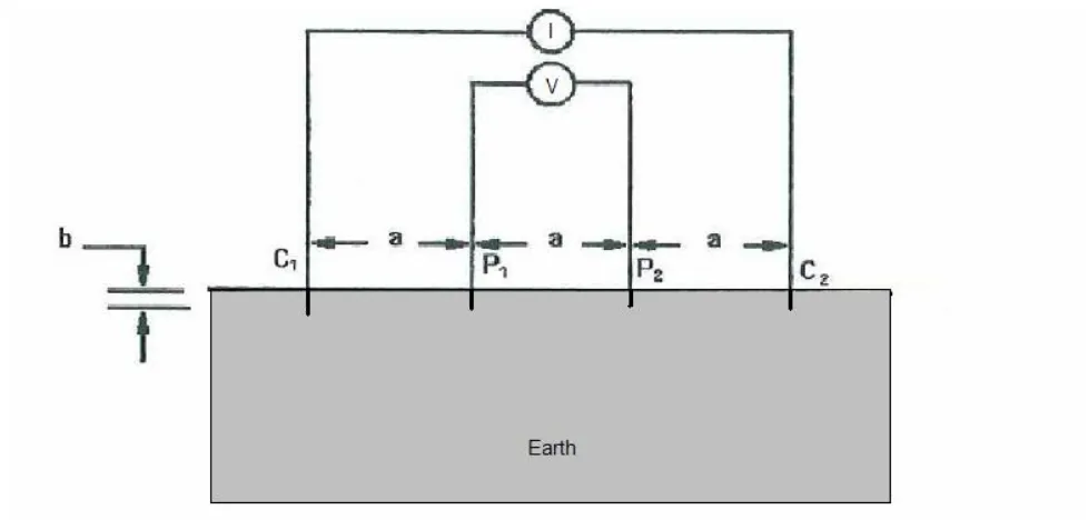
The Wenner Array Method

The Wenner array is one of the most commonly used methods of soil Resistivity testing and uses 4

electrodes as shown in figure 6. Four test spikes are inserted into the ground in a straight line at equal

distances ‘a’ and to a depth ‘b’ of less than 1/20 of ‘a’. A current signal, (AC, DC or complex) is injected via

the two outermost electrodes (C1 and C2), and then measurement of the resulting voltage signal is taken

across the two inner probes (P1 and P2). The instrument then returns a Resistance measurement, from which

ce

sis

Measured

R

A

Current

Injected

I

V

Voltage

Measured

v

Spacing

obe

a

m

sistivity

Apparent

tan

Re

)

(

)

(

Pr

)

(

Re

=

=

=

∆

=

Ω

=

ρ

To obtain the Resistivity of the soil at various depths, this test is repeatedly conducted as part of a traverse of

the site, I.e. at several probe spacings, as denoted by “a” in figure 6. The spacing of the probes, is altered

from close spacings (1m +), up to spacings of at least the radius or longest diagonal of the proposed earth

grid. An example of a range of probe spacings for a resistivity traverse is shown below in Table 1.

Resistivity Traverse – Site 123 – Wenner Array Probe Spacing

‘a’

1 2 4 8 16 32 64 128

Resistance Measured Ω

34.2 16.22 1.344 0.832 0.453 0.321 0.256 0.222

Table 1: Resistivity Traverse. Traverse of site indicating probe spacings of up to 128m

This method is the most effective, when the test equipment has limited power output or limited ability to

detect low voltage signals. This effectiveness is due to the ratio of received voltage per unit of transmitted

current. (source ENA EG1, 2006). As a drawback, the Wenner array requires the longest cable layout and

can also be time consuming due to each of the electrodes having to be moved, for each electrode spacing test.

Portable test equipment often specifies the use of the Wenner array, due to the limited power output available

from a Battery power supply within the test instrument. The user manuals for the Fluke 1625 and the

Megger DET/2, as specified in section 2.1.3, both specify the use of the Wenner array for Resistivity testing.

As this equipment was selected for use in this research project, the Wenner array has been used for all of the

Figure 6: Wenner Array. Probe layout and injected and measured signals.

5.1.2

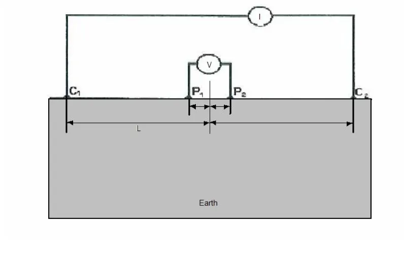
The Schlumberger Array Method

The Schlumberger array is similar to the Wenner array, as it also uses 4 electrodes and operates on the

injected current and measured voltage principle of the Wenner array. There are, of course, several major

differences with the Schlumberger array, namely the probe spacing requirements, the magnitude of injected

current and the magnitude of the voltage measured.

The Schlumberger array is an electrode configuration in which the spacing of the two potential electrodes

(P1 and P2) is less than one-fifth of the distance between the centre of the array and one current electrode

(L). The use of the Schlumberger array allows for reduced testing time, since the current electrodes are

moved four or five times for each move of the Voltage electrodes. The Schlumberger array is also considered

more accurate than the Wenner or Driven rod methods, provided a current source of sufficient power is used.

Where

ce

resis

Measured

R

m

probes

voltage

to

centre

from

Spacing

l

m

probes

current

to

centre

from

Spacing

L

m

sistivity

Apparent

tan

)

(

)

(

)

(

Re

=

=

=

Ω

=

ρ

(source: ENA EG1, 2006).

An example of a Schlumberger array is shown in figure 7.

Figure 7: Schlumberger Array. Probe layout and injected and measured signals .

5.1.3

The Driven Rod (3 Pin) Method

The Driven rod method is sometimes referred to as the three pin, or fall of potential method. This method, as

the name implies, uses only three electrodes in a configuration as shown in figure 8. The driven rod method

is suitable for use in areas of difficult terrain, or for proposed simple earthing arrays (i.e. Transmission line

structures). Similar to both the Wenner and Schlumberger arrays, a traverse is completed of the site, and the

resistance of the soil taken at varying distances.

From the resistance readings obtained, the resistivity of the soil can be calculated using:

Where

ce

resis

Measured

R

m

diameter

rod

Driven

d

m

soil

with

contact

in

rod

driven

of

Length

l

m

sistivity

Apparent

tan

)

(

)

(

)

(

Re

=

=

=

Ω

=

ρ

(source: ENA EG1, 2006).

A diagram of the Driven rod array is shown in figure 8.

Figure 8: 3 Pin Array. Probe layout and injected and measured signals

6.

Tests Conducted and Results Obtained

6.1

Introduction

As indicated in section 3.2, a schedule of tests was created to provide a logical, well though out plan of tests

to be conducted, in order to try and obtain as accurate and repeatable data as possible. The schedule of tests

was created as a “live” document as the findings of the initial tests, provided the reasoning for additional

tests to be completed. The full schedule of tests is attached to this document in appendix C, with an outline

of the creation process of the schedule of tests, as follows.

6.2

Initial Tests (Stage 1)

6.2.1

Site and Test Instrument Selection

Initially, the schedule of tests was created based on conducting a Resistivity Traverse at two different

locations, using the Wenner Array. These locations were selected as vacant parcels of land, well clear of any

fences, pipelines, power lines or other sources of potential interference. Numerous sources of information

relative to earth resistivity including ENA EG1: 2006 and IEEE:80 mention the need for careful selection of

sites clear of powerlines, pipelines, fences, etc which may influence test results.

Site 1 was selected in an area west of Caboolture, approx 1 Hr north of Brisbane, and site 2, selected just

outside of Pittsworth, approximately ½ Hr South West of Toowoomba. These sites were selected based on

their natural terrain, ease of access, and affiliation with the relevant property owners. Both sites were

carefully examined for evidence of buried pipelines, communications cables or other services, as well as

proximity to powerlines and other potential sources of interference. Due to each site being farmland which

has not undergone any type of development other than clearing for grazing and cropping, both sites were

assessed as suitable for the testing.

The initial tests were conducted using the Megger DET2/2 and the Fluke 1625 with the respective test leads

in a number of different layouts and at several electrode spacings. The use of two instruments were selected,

in order to compare readings between the selected instruments and highlight any inaccuracy that may be due

to coupling effects, or shortfalls of the test instruments themselves. For each resistivity traverse (series of

tests), the test probe spacing was selected in 1 metre increments up to 4m, then in 4m increments up to 16m,

then 8m increments up to the largest probe spacing of 32m. 32m was the largest possible spacing to be used

in this instance, due to the physical length of the test leads being 50 metres. Using a probe spacing of 32

metres, the distance from the centre of the array to each potential electrode (P1 and P2) is 16 metres, and

then a further 32 metres, to each current electrode, hence the maximum lead length required in this situation

6.2.2

Test Lead Layout

The selected test lead layouts were based on the orientation of the injected current signal leads with respect

to the measured voltage leads. Recall from the discussion in section 4.1.1 that the Wenner array uses four

electrodes, with the outermost two carrying the injected current signal, and the innermost two electrodes, the

measured voltage signal. As magnetic and capacitive coupling affects conductors in parallel, three logical

test lead orientations were derived. These layouts were: Leads at 90 degrees, Leads in parallel at 0 Degrees

and Leads in parallel at 180 Degrees. An aerial view diagram of these lead layouts are as shown below in

figures 9, 10 and 11.

Figure 11: Test Leads in Parallel (180°). Wenner array with current and voltage leads in parallel (180 degrees).

For both lead configuration 2 and 3 (conductors in parallel at 0° and 180°) the parallel sections of cable were

very carefully “strung” between the centre of the array and the potential electrodes, taking care to avoid any

twists in the cables. This was achieved by using wooden support structures at the relevant locations, to which

the current and voltage leads were fixed. Proximity of the leads was further ensured, by using a simple

clothes peg to ensure the conductor orientation was correct.. Figure 12 shows an example of the array

configuration for a test with leads in parallel. Note that this configuration did not require a wooden support in

the centre of the array due to the short parallel section of cable.

6.2.3

The Effects of Electrode Contact Resistance

Using these test lead configurations, the very early stages of testing, revealed a substantial variation in the

resistance readings displayed by each test instrument instrument, depending on the lead configuration. These

results were initially recorded, however the results obtained were highly inconsistent and largely

non-repeatable. Through further investigation, the test equipment manuals indicated the probable cause of the

variation in the results was due to a high contact resistance between the electrodes and the soil. The soil

under test was reasonably dry and hence the contact resistance between the electrode and the general mass of

earth was changing as the electrode was disturbed (even slightly) during alteration of the lead layout.

To overcome this variation due to the electrode contact resistance, a salt water solution was prepared, and a

small amount applied to each electrode, to negate these contact resistance effects. Repeat testing with the salt

water solution applied to all electrodes, obtained much more stable and repeatable results, and hence this

method was then adopted for all future testing to be conducted. The quantity of the salt water solution

applied to each electrode was kept to an absolute minimum, as the conductive properties of the soil would be

affected considerably, if large amounts of solution were applied, particularly at close probe spacings.

6.2.4

Information Recorded During Each Test

For each of the tests conducted, readings of the Injected Current, Measured Voltage, Displayed Resistance

and Signal Frequency, were recorded. In order to accurately record the variation in these parameters, the

careful selection of additional test instruments was required.

The instruction Manuals for the Megger DET2/2 and the Fluke 1625 indicate the injected current signal is

alternating DC, at various frequency ranges (as set by user). Based on an alternating DC current signal being

injected, the measured voltage signal will also be an alternating DC voltage, and hence, the theoretical

In order to measure what is therefore effectively a square wave, a True RMS multimeter and Current clamp

meter were selected. True RMS is stated as a specific method of measuring the RMS, or “DC Equivalent”

value of a signal. This method results in the most accurate RMS value regardless of the shape of the

waveform. Other methods of measuring RMS values exist, such as the rectifier or mean absolute deviation

method; however, these methods are accurate only for sine wave signals. Source: National Instruments,

2009

Consideration was also given to the accuracy of the Multimeter and Clamp Meter for measurement of higher

frequency signals. The injected signals were, as previously stated, alternating DC signals between

100-150Hz (depending on desired setting). The accuracy specifications for the Multimeter and Clamp Meter are

attached in appendix D, and show an accuracy of +/- 1% for sinusoidal signals up to 1kHz for the multimeter

and +/- 2% for signals up to 2kHz, for the clamp meter. On initial inspection, these specifications, indicate

good accuracy for signals in the expected frequency range (100-150Hz) , however if the injected signal were

considered as series of sinusoidal components, I.e. a Fourier series, the issue of accuracy with respect to

frequency, soon became evident.

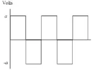
Fourier’s theorem states that any periodic signal can be decomposed into an infinite series of sine and cosine

functions. For a square wave as shown in Figure 13, the Fourier series can be described as:

K

7

,

5

,

3

,

1

)

sin(

1

=

+

∑

n

for

t

n

n

a

ω

Where ω0 is the fundamental frequency, and a is the DC component, or average DC offset.

Source: Facstaff, 2009.

For the Earth test signals of interest, it was assumed that the offset DC component was zero, (hence a=0) and

the waveform was symmetrical about the x axis. The stated default frequency for the Fluke 1625 is 111 Hz,

so the Fourier components of this signal can be calculated using the above equation. The resulting theoretical

frequency components are as shown in table 2.

Multiple Of Fundamental Frequency (111Hz) 1 (111Hz) 3 (333Hz) 5 (555Hz) 7 (777Hz) 9 (999Hz) 11 (1221Hz)

Magnitude Present In Signal

(multiple of fundamental amplitude)

1 1/3 1/5 1/7 1/9 1/11

From table 2 it can be seen, for example that the 11th harmonic component of the Fourier series (1221 Hz

component), the magnitude will be 1/11 of the peak value of the fundamental component. If the peak of the

fundamental measured signal is 50mV for example, the peak value of the 11th harmonic component will be

approximately 4.54mV, or ≈9% of the original signal. Attenuation of these higher frequency components would therefore lead to considerable inaccuracy in the results obtained.

The Manufacturers data for the Fluke 179 indicates that while accuracy of signals >1kHz is not specified, the

relative accuracy of a non-sinusoidal waveform is accounted for in a footnote to the table of specifications.

This states that: For non-sinusoidal waveforms accuracy, add -(2% reading + 2% full scale) typical.

Therefore the overall accuracy of the Fluke 179 can be considered as 3%, comprised of 1% accuracy for AC

signals up to 500Hz, plus the additional 2% for non sinusoidal waveforms.

Similarly, the Hioki 3283 states an accuracy of 2% for signals up to 2kHz, and the meter is stated as a True

RMS instrument, therefore the accuracy should be sufficient for this purpose.

Based on the requirements for the use of True RMS equipment and the frequency accuracy considerations

above, the instruments for measurement of the required parameters of the test signals, were selected as:

• Injected Current: Hioki 3283 High accuracy clamp meter. Resolution: 0.1mA True RMS meter

• Measured Voltage. Fluke 179 III Multimeter. Resolution 0.1mV, True RMS Multimeter

• Resistance– Taken directly from the readout of the Earth testing device.

• Frequency of the injected signal. Fluke 179 III Multimeter. Resolution 0.1 Hz, True RMS Multimeter

6.2.5

Calculation of Resistivity from Results Obtained

As defined in section 4.1.1, Soil Resistivity from a Wenner array test layout, can be calculated by using the

6.3

Considerations of Test Current Waveform Vs Power System Waveform

From section 6.2.4, the injected current waveform has been found as an alternating DC signal, which then

raises the question of accuracy in terms of AC current propagation through the same soil under test. Soil

Resistivity tests are conducted to establish the resistive properties of the soil, and therefore the use of a DC

signal is appropriate for such a purpose, however, it seems little or no consideration has been given to the

propagation of AC sinusoidal current through the same soil. The soil resistivity results obtained by using an

alternating DC test signal may not accurately represent the flow of current through the same soil, for a 50Hz

current signal.

If we consider the soil under test in a similar manner to a simple conductor, or group of conductors, the soil

may exhibit different electrical properties such as inductive or capacitive effects, under different

circumstances. It appears that significant research has been conducted into the dielectric properties of soil,

and the findings of others (see references) appear to indicate the presence of frequency dependent

characteristics within the soil.

An example of such a finding is outlined by Van Dam et al in the paper entitled “Methods for prediction

of soil dielectric properties: a review”. The paper outlines the electrical and magnetic properties of soils,

based on the nature and dielectric properties of the soil, and how these properties are dependant on

frequency. One notable quote from this paper is the statement “The interaction of electromagnetic energy

with matter is affected by the characteristics of the material and by the frequency of the electromagnetic

energy”. Boydell et al, indicate a similar discussion, detailing that the “Soil Elelctrical Conductivity

properties are dependant on the electrolyte concentration and its connectivity or continuity within the

profile”.

The research into the electrical properties of soils is outside the scope of this research paper, however the

intent of the above citations are to raise awareness to the reader, of such frequency dependant effects. Further

investigation into the propagation of DC and AC current through the same soil strata is a possible area of

6.3.1

Results Obtained From Initial (Stage 1) Testing

Using the specifications above the initial tests and required calculations were carried out. The results of these

tests have been presented in the following sections in graphical form, for ease of perusal, and comparison of

results. The presentation of results has been based on the following Characteristics:

• Comparison of the Resistivity curves as calculated from the measured resistance (instrument reading), for each of the test lead layout patterns.

• Comparison of the Resistivity curves as calculated from the resistance readings and as calculated from the measured V and I signals for each test lead layout

The full table of Soil Resistivity results from which these graphs have been produced, have been included in

6.3.2

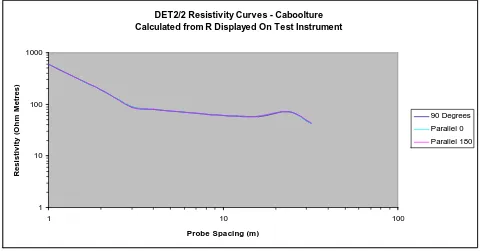
Resistivity Curves Calculated From Measured Resistance – Caboolture Site

DET2/2 Resistivity Curves - Caboolture Calculated from R Displayed On Test Instrument

1 10 100 1000

1 10 100

Probe Spacing (m)

R e s is ti v it y ( O h m M e tr e s) 90 Degrees Parallel 0 Parallel 180

Figure 14: Resistivity Curves. DET2/2 - Caboolture Site: Resistivity curves as calculated from resistance readings- Megger DET2/2 instrument at Caboolture site.

Fluke 1625 Resistivity Curves - Caboolture Calculated from R Displayed On Test Instrument

1 10 100 1000

1 10 100

Probe Spacing (m)

R es is ti v it y ( O h m M e tr es) 90 Degrees Parallel 0 Parallel 180

6.3.3

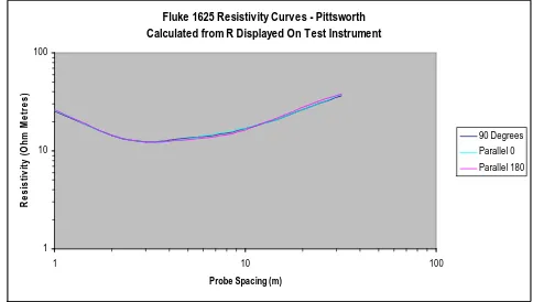
Resistivity Curves Calculated From Measured Resistance – Pittsworth Site

DET2/2 Resistivity Curves - Pittsworth Calculated from R Displayed On Test Instrument

1 10 100

1 10 100

Probe Spacing (m)

R e s is ti v it y ( O h m Me tr e s) 90 Degrees Parallel 0 Parallel 180

Figure 16: Resistivity Curves. DET2/2 - Pittsworth Site: Resistivity curves as calculated from resistance readings- Megger DET2/2 instrument at Pittsworth site.

Fluke 1625 Resistivity Curves - Pittsworth Calculated from R Displayed On Test Instrument

6.3.4

Resistivity Curves as Calculated From Measured Resistance Vs Measured

Voltage and Current: Megger DET2/2 Instrument – Caboolture Site.

Figure 18: Resistivity Curves. Megger DET2/2 - Caboolture Site: Resistivity curves as calculated from Resistance readings Vs measured Current and Voltage.

DET2/2 Resistivity Curves - Caboolture - Test leads @90 degrees

1 10 100 1000

1 10 100

Probe Spacing (m)

R e s ist iv it y ( O h m M e tr es)

Calc From R Calc From V/I

DET2/2 Re sistiv ity Curv e s - Caboolture - Te st le ads Paralle l @ 180 de gre e s

1 10 100 1000

1 10 100

Probe Spacing (m)

R es ist iv it y ( O h m M et res)

Calc From R Calc From V/I DET2/2 Resistivity Curves - Caboolture - Test leads Parallel @ 0 degrees

1 10 100 1000

1 10 100

Probe Spacing (m)

R e s ist iv it y ( O h m M e tr es)

6.3.5

Resistivity Curves as Calculated From Measured Resistance Vs Measured

Voltage and Current: Fluke 1625 Instrument – Caboolture Site.

Fluke 1625 Resistivity Curves - Caboolture - Test leads @ 90 degrees

1 10 100 1000

1 10 100

Probe Spacing (m)

R es is ti v it y ( O h m M e tr e s)

Calc From R Calc From V/I

Fluke 1625 Resistivity Curves - Caboolture - Test leads Parallel @ 0 degrees

1 10 100 1000

1 10 100

Probe Spacing (m)

R e s is ti v it y ( O h m M e tr e s)

Calc From R Calc From V/I

Fluke 1625 Resistivity Curves - Caboolture - Test leads Parallel @ 180 degrees

100 1000

e

tr

6.3.6

Resistivity Curves as Calculated From Measured Resistance Vs Measured

Voltage and Current: Megger DET2/2 Instrument – Pittsworth Site

Figure 20: Resistivity Curves. Megger DET2/2 - Pittsworth Site: Resistivity curves as calculated from Resistance readings Vs measured Current and Voltage.

DET2/2 Resistivity Curves - Pittsworth - Test leads @90 degrees

1 10 100 1000

1 10 100

Probe Spacing (m)

R es ist iv ity ( O h m M e tr e s)

Calc From R Calc From V/I

DET2/2 Re sistiv ity Curv e s - Pittsworth - Te st Le ads Paralle l @ 0 de gre e s

1 10 100 1000

1 10 100

Probe Spacing (m)

R e s is ti v it y ( O h m M e tr es)

Calc From R Calc From V/I

DET2/2 Resistivity Curves - Pittsworth - Test Leads Parallel @ 180 degrees

1 10 100 1000

1 10 100

Probe Spacing (m)

R e s is ti v it y ( O h m M et re s)

6.3.7

Resistivity Curves as Calculated From Measured Resistance Vs Measured

Voltage and Current: Fluke 1625 Instrument – Pittsworth Site

Flukle 1625 Resistivity Curves - Pittsworth - Test leads @90 degrees

10 100

1 10 100

Probe Spacing (m)

R es is ti v it y ( O h m M e tres)

Calc From R Calc From V/I

Fluke 1625 Resistivity Curves - Pittsworth - Test Leads Parallel @ 0 degrees

10 100

1 10 100

Probe Spacing (m)

R es is ti v it y (O hm M e tr e s)

Calc From R Calc From V/I

Fluke 1625 Resistivity Curves - Pittsworth - Test Leads Parallel @ 180 degrees

100

e

6.4

Discussion of Initial (Stage 1) Test Results

6.4.1

Test Lead Coupling and the Resistance Indicated by the Test Instrument

With respect to the Resistivity traverses conducted as per section 5.3, the effect of test lead coupling does not

appear to have significant effect on the Resistance displayed by the test instruments. Based on the

information displayed in figures 14 to 17, the effects of test lead coupling, does not appear to be significant,

for tests conducted at spacing up to and including 32 metres. These Resistivity curves show slight variation,

and inspection of the results obtained, (Refer Appendix E) reveals the relatively small magnitude of this

variation. The cause of the variation could be attributed to coupling effects only, however consideration must

be given to other external influences that may have been present. Several external factors which may have

been present and therefore require consideration are:

• Disturbance of the test electrodes during alteration of the test lead Layouts. Slight movement of the electrodes is unavoidable when changing the layout of the test leads to the 3 predefined

configurations. As previously discussed, a salt water solution was used to overcome the effects of

electrode contact resistance, however this does not guarantee the properties of the contact area will

remain identical for each test, particularly when the electrode is disturbed between tests.

• Transferral of leads between instruments for each lead configuration. With the test leads set up for each lead configuration, each test was completed using both instruments, before alteration of the

leads or electrodes to the next required configuration. By transferring the leads between instruments,

the connections between the test leads and the instrument are altered, and therefore may lead to

slight variation in the test results.

Taking into account the inaccuracies that may have been introduced by the above factors, variation in the

results recorded, still appears to be present. The variation in the Resistance readings obtained, while small in

nature, does appear to increase, as probe spacing is increased. A summary of the results obtained from both

sites, for probe spacing of 1 and 32 metres has been included below in table 3, to outline the variation present

between the different tests. The results obtained for 1 metre spacing show a very small percentage variation

in resistance reading between the 90 degree test lead configuration and the parallel test lead configurations of

zero and 180 degrees. Comparison of these results with the results of tests conducted at 32 metre probe

spacing, clearly reveals the larger percentage variation in resistance readings obtained. As coupling effects

would reasonably be expected to increase, with an increase in the parallel section of test lead, tests conducted

Further investigation into the effect of coupling on the resistance displayed, appears warranted as the test

probe spacing is increased above 32 metres. As previously indicated, the equipment available for these tests

had a test lead length of approximately 50 metres, hence testing with probe spacing greater than 32 Metres

was unachievable using the equipment available at the time of the initial tests.

Caboolture Site

Lead Orientation Instrument

R Measured 1m Variation From 90° Reading R Measured 32m Variation From 90° Reading

90 Degrees DET2/2 95 N/A 0.211 N/A

Parallel 0 DET2/2 95.1 0.105% 0.213 0.947%

Parallel 180 DET2/2 95.1 0.105% 0.216 2.37%

90 Degrees Fluke 1625 95 N/A 0.21 N/A

Parallel 0 Fluke 1625 95 0 % 0.22 4.7%

Parallel 180 Fluke 1625 95.1 0.105% 0.22 4.7%

Pittsworth Site

Lead Orientation Instrument

R Measured 1m Variation From 90° Reading R Measured 32m Variation From 90° Reading

90 Degrees DET2/2 4.12 N/A 0.175 N/A

Parallel 0 DET2/2 4.17 1.21% 0.187 6.86%

Parallel 180 DET2/2 4.21 2.18% 0.182 4%

90 Degrees Fluke 1625 4.08 N/A 0.18 N/A

Parallel 0 Fluke 1625 4.13 1.23% 0.19 5.55%

Parallel 180 Fluke 1625 4.17 2.21% 0.19 5.55%

Table 3: Variation in Resistance readings for probe spacing of 1metre and 32 metres

6.4.2

Test Lead Coupling and the Measured Voltage and Current Signals

On inspection of Figures 18 to 21, the effects of test lead coupling appears to become more evident when

considering the True RMS Voltage and Current signals measured by the Fluke 179 and Hioki 3283

It is not accurate to say that all of the variation we have found can be attributed solely to the effects of test

lead coupling, however, the results for both sites and both instruments, indicate the effects of coupling are

indeed present. External factors such as environmental noise must be considered, however, are assumed to be

non-significant in this case, based on the selection of the test sites. Because of the careful selection of the test

sites as areas well clear of any infrastructure such as fences, powerlines, pipelines, etc. any environmental

noise present, is therefore considered as normal or “background” noise, as would be encountered in almost

any situation.

6.5

Further Testing Based on Results of Initial Tests. (Stage 2 Tests)

Using the information obtained from the results of the initial (stage 1) tests, further testing was deemed

necessary. The intent was to more accurately determine the coupling effects on the injected current and

measured voltage signals for tests conducted using a large probe spacing, in this case, 32 Metres.

Using a digital scope meter (a digital version of a Cathode Ray Oscilloscope) and the Fluke 1625 Instrument,

a Wenner Array with probe spacing of 32 Metres was prepared. The scope meter selected was a Philips

PM97 Scopemeter, based on availability through Downer EDI Engineering.

Using this equipment, a Resistivity test was conducted using each of the 3 test lead layout configurations,

and the Resistance displayed together with the waveform of the injected current and voltage signals were

obtained. The injected current and measured voltage waveforms were obtained using the “hold” function of

the scope meter, and recorded using a Digital Camera. The Philip