This is a repository copy of Low flow controls on stream thermal dynamics. White Rose Research Online URL for this paper:
http://eprints.whiterose.ac.uk/122730/ Version: Accepted Version
Article:
Folegot, S, Hannah, DM, Dugdale, SJ et al. (9 more authors) (2018) Low flow controls on stream thermal dynamics. Limnologica - Ecology and Management of Inland Waters, 68. pp. 157-167. ISSN 0075-9511
https://doi.org/10.1016/j.limno.2017.08.003
© 2017 Elsevier GmbH. This manuscript version is made available under the CC-BY-NC-ND 4.0 license http://creativecommons.org/licenses/by-nc-nd/4.0/
[email protected] https://eprints.whiterose.ac.uk/ Reuse
Items deposited in White Rose Research Online are protected by copyright, with all rights reserved unless indicated otherwise. They may be downloaded and/or printed for private study, or other acts as permitted by national copyright laws. The publisher or other rights holders may allow further reproduction and re-use of the full text version. This is indicated by the licence information on the White Rose Research Online record for the item.
Takedown
If you consider content in White Rose Research Online to be in breach of UK law, please notify us by
Accepted Manuscript
Title: Lowßow controls on stream thermal dynamics
Authors: Silvia Folegot, David M. Hannah, Stephen J. Dugdale, Marie J. Kurz, Jen Drummond, Megan J. Klaar, Joseph Lee-Cullin, Toralf Keller, Eug`enia Mart´õ, Jay P. Zarnetske, Adam S. Ward, Stefan Krause
PII: S0075-9511(16)30050-0
DOI: https://doi.org/10.1016/j.limno.2017.08.003
Reference: LIMNO 25603
To appear in:
Received date: 22-6-2016
Revised date: 22-5-2017
Accepted date: 7-8-2017
Please cite this article as: Folegot, Silvia, Hannah, David M., Dugdale, Stephen J., Kurz, Marie J., Drummond, Jen, Klaar, Megan J., Lee-Cullin, Joseph, Keller, Toralf, Mart´õ, Eug`enia, Zarnetske, Jay P., Ward, Adam S., Krause, Stefan, Lowßow controls on stream thermal dynamics.Limnologica https://doi.org/10.1016/j.limno.2017.08.003
Low flow controls on stream thermal dynamics
Silvia Folegot1, David M. Hannah1, Stephen J. Dugdale1, Marie J. Kurz2,3, Jen Drummond4, Megan J. Klaar1,5, Joseph
Lee-Cullin6, Toralf Keller2, Eugènia Martí4, Jay P. Zarnetske6, Adam S. Ward7 and Stefan Krause1
1School of Geography, Earth and Environmental Sciences, University of Birmingham, Edgbaston, Birmingham, B15 2TT U.K. 2Department of Hydrogeology, Helmholtz Centre for Environmental Research-UFZ, Leipzig, Germany
3Patrick Center for Environmental Research, The Academy of Natural Sciences of Drexel University, Philadelphia, Pennsylvania, USA 4Centre for Advanced Studies of Blanes (CEAB-CSIC), Blanes, Girona, Spain
5School of Geography, University of Leeds, LS2 9JT Leeds, U.K.
6Department of Earth and Environmental Sciences, Michigan State University, East Lansing, Michigan, USA 7School of Public and Environmental Affairs, Indiana University, Bloomington, Indiana, USA
Correspondence to: Silvia Folegot ([email protected])
Abstract
Keywords: sediment-water interface, water level fluctuations, temporal-spatial temperature patterns, FO-DTS, macrophytes shading, habitat complexity.
1. Introduction
Temperature is a master water quality variable driving physical, chemical, and biological processes in aquatic ecosystems by directly influencing metabolic rates, physiology and life-history traits of aquatic organisms, as well as their abundance and distribution (Webb, 1996; Constantz, 1998; Bogan et al., 2003; Caissie, 2006; Webb et al., 2008). Stream water temperature is dynamic over space and time (Poole and Berman, 2001), and is influenced by numerous natural variables and eco-hydrological processes, including solar radiation, air temperature, heat transfer at the air-water interface, precipitation, riparian vegetation shading, surface water inflows, and groundwater and streambed heat exchanges (Constantz, 1998; Bogan et al., 2003; Johnson, 2004; Arrigoni et al., 2008; Webb et al., 2008; Garner et al., 2015a; Hannah and Garner, 2015). In particular, the streambed, identified as an important heat source and sink (Evans et al., 1998; Hannah et al., 2004), can significantly affect the
river’s energy budget both temporally and spatially (Evans et al., 1998), influencing water
column temperatures. Natural temporal fluctuations in surface and streambed water temperature are observed on a diel and annual cycle (Caissie, 2006), while spatially, temperatures generally increase along the longitudinal dimension. However, discontinuities, both of natural and anthropogenic origin can interrupt the longitudinal thermal profile (Fullerton et al., 2015). At the micro-scale, morphological in-stream structures like riffle-pool sequences create spatial temperature heterogeneity, supporting diverse communities and providing refuge from extreme temperatures, especially during summer (Hester et al., 2009; Dallas and Rivers-Moore, 2011). Although temperature variations occur naturally, river flow and thermal regimes have been profoundly altered by both climate change and human interventions, e.g. dams and water withdrawals, on the hydrological cycle (Döll and Zhang, 2010; Schneider et al., 2013; Laizé et al., 2014), with potential severe impacts on freshwater ecosystems and biodiversity (Bates et al., 2008; Bond et al., 2008; Poff and Zimmerman, 2010; Vörösmarty et al., 2010).
Water depth together with discharge and velocity directly influences and regulates the distribution and growth of aquatic flora (Riis and Biggs, 2003; Franklin et al., 2008; Bornette and Puijalon, 2011). Macrophyte communities play a key role in unshaded streams (Riis and Biggs, 2003), by increasing physical and biological diversity, and by contributing to habitat structure and ecological functioning of these systems (Warfe and Barmuta, 2006; Thomaz and Cunha, 2010). While stable flows favour macrophyte biomass (Mebane et al., 2014), the increased number and frequency of hydrological disturbance events, such as floods and droughts, can significantly alter the composition and abundance of aquatic macrophyte communities (Riis and Biggs, 2001; Riis and Biggs, 2003; Stromberg et al., 2005), causing biomass destruction, and habitat structure change (Grime, 1979). Under this constraint, plant species with a greater resistance and/or resilience usually dominate (Riis et al., 2008), whereas others, such as Ranunculus species, only occupy channel areas with permanent flow (Westwood et al., 2006). As a result, during droughts, the channels of ephemeral or perennial streams experiencing severe drying can be invaded and colonized by resistant and/or amphibian or riparian plant species (Bunn and Arthington, 2002; Lake, 2003), a process called terrestrialization (Westwood et al., 2006; Holmes, 1999). Strictly aquatic macrophytes (Schuyler, 1984) and non-aquatic forms possess different shading abilities that are quite influential for both water and streambed temperatures. Non-aquatic forms in particular, being characterized by more competitive growth forms (e.g. tall or broad-leafed species; Bornette and Puijalon, 2011), have highly variable shading effects on surface water and streambed sediments. Therefore, water level fluctuations due to drought conditions can influence aquatic vegetation coverage and indirectly, stream temperature regimes. However, to our knowledge, no previous high spatio-temporal resolution studies of the combined impact of both water level and vegetation coverage on temperatures at the channel bed and in the water column have been carried out.
Direct in situ studies of water level impacts on the thermal regime of natural channels can be challenging technically and logistically because of their high spatial and temporal complexity. The use of distributed fibre optic monitoring solutions allow for the possibility to investigate stream thermal regimes continuously in both time and space (Selker et al., 2006b; Tyler et al., 2009). In this way, high spatial and temporal stream temperature variability can be detected, resulting in improved monitoring and assessment of stream thermal regimes. Manipulating water levels in a flume experimental set-up allows for the isolation and alteration of the key variables of interest under controlled conditions, although at a smaller physical scale (Mosley and Zimpfer, 1978).
at unprecedented spatial and temporal scales. We hypothesised that: i) surface water warming would be inversely associated with water depth with temperatures in the deeper flumes being more effectively buffered by both the water column and broader co-evolving vegetation coverage than in shallower flumes; ii) spatial temperature patterns would be more pronounced in the shallowest flume with extreme temperature values (maximum and minimum streambed and surface water temperature values) varying more than average temperatures; and iii) the impact of meteorological variability, especially changes in air temperature and solar radiation, would be more marked for shallower water depths.
2. Material and methods
2.1 Site description
Our experiment used three outdoor flumes at Fobdown Watercress Farm, near New
Alresford, Hampshire, U.K. (51°06 08.57 N, 1°11 06.33 W, 99 m asl; Figure 1).
Approximate location of Figure 1
The experiment ran from ~ 16:00 23-04-2014 to ~14:00 25-04-2014. Average air temperature for the month of April was 10.0 °C (Alice Holt Lodge UK Met Office weather station, ~ 30 km away from study site), with a peak of 17.5 °C on the 21-04-14. The minimum of 2.1 °C was registered the 24-02-16. Daily average precipitation was 0.2 mm with a maximum of 13.4 mm on the 25-04-14 (Figure 2).
Approximate location of Figure 2
The aluminium flumes had dimensions of 15 m length and 0.5 m width, with walls of 0.5 m (Figure 1). Water supply for the flumes was provided from a groundwater well with a constant temperature of 10.1 °C. Water quality parameters (temperature, electric conductivity and dissolved oxygen) were monitored continuously to ensure stationary water quality boundary conditions throughout the experiment. Groundwater (GW) was pumped at a constant rate into a feeder tank of 80 L capacity, from where it was subsequently distributed to the flumes using a network of pipes. Different water levels were obtained by regulating the water intake and outflow for each flume separately, and water levels in the pools were set to
25, 10 and 7 cm in the three flumes, respectively (flumes are hereafter referred to as ‘1_25
cm’, ‘2_10 cm’ and ‘3_07 cm’). The three water levels were representative of different levels
of drought severity, with flume 1_25 cm representing close to normal flow conditions for southern UK chalk streams, flume 2_10 cm summer low flow conditions and 3_07 cm severe drought conditions. Steady state conditions were maintained throughout the experiment.
in the flumes were calculated by subtracting the flume-averaged depth to water and the sediment thickness at each grid cell from the total flume wall height.
Approximate location of Table 1
Vegetation in the flumes was introduced artificially using ~ 10 cm 5-rooted fragments of Ranunculus penicillatus subsp. pseudofluitans spaced at 2 m intervals, and was allowed to evolve naturally since the flumes’ installation in August 2013. Ranunculus penicillatus subsp. pseudofluitans (Syme) S.D. Webster, is a divergent, fine-leaved, submerged aquatic macrophyte, typically found in English chalk streams where it is generally the dominant species. At the time of the experiment, the flumes’ vegetation represented a climax community that had developed for 8 months after flume installation according to the water level present in each flume. The vegetation cover (%) during the experiment was estimated by photo surveys taken every 1.5 m along the flumes.
Sediment thickness, water depth and vegetation coverage surveys were interpolated using Ordinary Kriging in ArcGIS (ESRI, 2011). Interpolations of all three spatial parameters (sediment thickness, water depth and vegetation coverage) resulted in rasters of 1.9 cm grid cells. These data were further analysed using the Spatial Analysis toolbox in ArcGis (ESRI, 2011) to evaluate spatial patterns in average, variance, minimum and maximum temperature ranges and as well as spatial correlations between parameters (using Band Collection analysis).
2.2 Field instrumentation
2.2.1 Surface water temperature monitoring
flow of a riffle (Green, 2005). Therefore, a blockage across the flume by macrophytes could be seen as being a pseudo-riffle (Green, 2005). Spot surveys confirmed that surface water temperatures did not stratify.
Analysis and processing of data were performed using the R statistical computing and graphic environment (R Core Team, 2013).
2.2.2 Streambed water temperature monitoring
To investigate spatial patterns of streambed temperature continuously at high spatio-temporal resolution, FO-DTS technology was applied along a complex geometrical setup (Figure 1). In recent years, distributed temperature sensing technology based on Raman backscatter from fibre optic cables has been widely adopted for extensive environmental applications (Selker et al., 2006a; Tyler et al., 2009; Briggs et al., 2012; Krause et al., 2012; Sebok et al., 2015). The measurement principle of FO-DTS is based on the analysis of the backscatter properties of a light pulse emitted from the DTS unit that travels through an optical fibre. The observed ratio of Stokes/anti-Stokes backscatter is used to quantify temperature at high sampling resolution (up to 12.5 cm) along fibre-optic cables (up to several km in length). Measurement precision depends on distance from the light source and on the integration time, so points further from the DTS unit have fewer photons observed and will need greater integration times to achieve desired precision (Selker et al., 2006a). Assuming robust calibration procedures, DTS systems with 1 m spatial resolutions along cables of up to 5 km have been reported to provide precision of the order of 0.1 C for integration times of 60 seconds (Selker et al., 2006a; van de Giesen et al., 2012).
Approximate location of Table 2
For the experiment, a fibre-optic cable within a stainless-steel tube was deployed at the sediment surface water interface of the three flumes using a double-looped configuration as indicated in Figure 1. For flume 1_25 cm, 2 transects of FO-DTS cable were deployed at the streambed surface (cable failure in the second loop), whereas for flume 2_10 cm and flume 3_07 cm, 4 transects were used. The cables were fixed to the streambed using flat stones to keep them in position. Nevertheless, exposure of the cable to the air could not be completely prevented, particularly in the shallowest sections. Sections of data where the cable detached from the sediment surface were discarded and considered as missing values (NAs) in the subsequent analysis. Similarly, the most up-stream and down-stream measuring points where the cables entered and exited the flumes (which may have been influenced by air temperature), were excluded from the data analysis. The number of points that had to be discarded for each transect varied between different DTS sections among flumes (Table 2). Because of the presence of a cable coil at the upstream end of the flume, the most upstream DTS sampling point taken into consideration for flume 1_25 cm was 1 m further downstream than in the other two flumes.
insensitive 50-µm multimode fibres were bedded in a gel, and the stainless-steel tube (SS 304) was not encapsulated. An ULTIMA-S ™ (Silixa, Elstree, UK) DTS instrument was used with a sampling resolution of 12.5 cm that offers a spatial resolution as fine as 30 cm. FO-DTS monitoring was carried out in single-ended mode with alternating measurement directions of the light pulse as described in Krause & Blume (2013)in order to preserve the best possible resolution of the spatial temperature patterns. To account for signal drift and offset a dynamic calibration was defined (Hausner et al., 2011) and for this, ~15 m reference sections of the fibre-optic cable were installed in a constant temperature ice bath. To avoid preferential heat transport, the cable was fully covered with iced water; cable contact with the walls of the ice container was avoided throughout the experiment. Temperature measurements were averaged at 30-second intervals for the duration of the experiment, this means that the time interval between measurements from the same channel was one minute. Streambed temperature data were analysed using the package matrixStats (Bengtsson, 2015) of the statistical software R (R Core Team, 2013) and daily mean, variance, minimum and maximum temperatures were obtained for each sampling day and plotted using the ggplot2 package (Wickham, 2009).
2.3 Predictions of surface water temperature variations
In order to ensure that observed changes in surface water temperature between the inflow and outflow in each of the flume were in line with theoretical expectations, and not due to solar warming of the instrumentation, a simple Lagrangian deterministic approach similar to that described by Garner et al (2014) was used to model water temperature within the flumes. Equations used to compute heat inputs due to solar radiation, net longwave radiation, latent heat and sensible heat were derived from those given in Boyd and Kasper (2003). As input meteorological data was not available directly on-site, input meteorological parameters were collected from the nearest (~ 30 km) UK Met Office weather station, located in Southampton (Met Office, 2006). The model calculates the temperature of a parcel of water of 0.126 m (length equal to the chosen spatial resolution of the DTS instrument) by 0.5 m (width equal to the width of the flume) as it moves through the flume. The model assumes that water within the flume is well mixed. Simplified streambed morphology was assumed and depth was the averaged depth in each flume (Table 3). The residence time of each parcel within the flume was ~5 hours.Vegetation coverage was not taken into account. Water parcels were ‘released’ on an hourly basis for the period 23-04-14 16:00 to 24-04-14 13:00, and the temperature of each parcel computed hourly as it transited the flume. The magnitude of warming of a parcel was computed by subtracting the modelled temperature of water at the outflow of the flumes from the inflow (inflow temperature given by the temperature data logger placed in the first pool in flume 2_10 cm). The rate of predicted changes was used to confirm that observed variations were in line with theoretical expectations.
3. Results
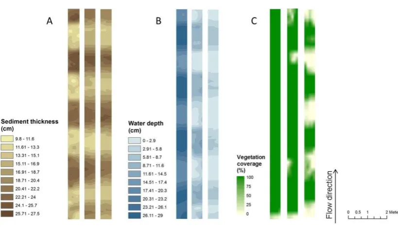
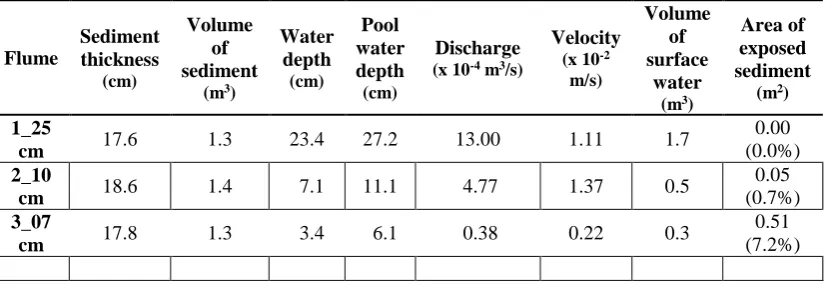
Sediment thickness and water depths for the three flumes are shown in Figure 3 A and B. The average sediment thickness of each of the flumes was 17.6, 18.6 and 17.8 cm for flumes 1_25 cm, 2_10 cm and 3_07 cm, respectively. Average flume water depths were 23.4, 7.1 and 3.4 cm for flumes 1_25 cm, 2_10 cm and 3_07 cm, respectively (Table 3). The pool-riffle-pool sequences formed by the sediments in the flumes comprised 4 pools per flume with an average water depth of 27.2, 11.1 and 6.1 cm for flumes 1_25 cm, 2_10 cm and 3_07 cm, respectively. All sediments were submerged in flume 1_25 cm, while 0.05 m2 of sediment was exposed to the air in flume 2_10 cm (0.7% of the total flume surface area) and 0.52 m2 (7.2% total area) was exposed in flume 3_07 (Table 3).
Approximate location of Table 3
3.2 Vegetation coverage
Vegetation coverage in the 3 flumes is shown in Figure 3 C. Total vegetation coverage for flume 1_25 cm was 96.7% (7.01 m2), including 95.3% coverage by aquatic vegetation (R. pseudofluitans) and 1.38% by emergent herbaceous plants. Un-vegetated areas consisted of open water, mainly near the flume inlet. In flume 2_10 cm, total vegetation coverage was 90.6% (6.57 m2), including 88.6% aquatic vegetation and 2.1% terrestrial cover. The remaining un-vegetated area consisted of a small area of bare sediments (0.05 m2, 0.7% of total area) and of shallow surface water (0.63 m2, 8.7% of total area). In flume 3_07, the total vegetated cover was only 4.07 m2 (56% of total area), including 51.5% aquatic vegetation and 4.5% non-aquatic plants. Bare, exposed sediments covered a surface area of 0.52 m2 (7.2% of the total area), and un-vegetated water made up the remaining 2.67 m2 (36.8% of total area). Spatial correlation using Band Collection analysis between vegetation coverage (without distinction between strictly aquatic and non-aquatic forms) and water level rasters within each flume revealed no correlation for flume 1_25 cm, increasing to 0.46 (p < 0.001) for flume 2_10 cm and 0.85 (p < 0.001) for flume 3_07 cm.
3.3 Influence of water depth on surface outflow temperatures
Water entering the flumes had a constant temperature of 10.1 C (± 0.07 °C) throughout the duration of the experiment (Figure 4 A). Mean (±standard deviation) of surface outflow temperatures recorded by the temperature loggers placed at the end of each of the flume was 10.5±0.1, 10.5±0.1, 10.5±0.2 C for flumes 1_25 cm, 2_10 cm and 3_07 cm respectively on 23-04-14, 10.7±0.5, 10.7±0.4, 11.1±1.1 C for flumes 1_25 cm, 2_10 cm and 3_07 cm respectively on 24-04-14 and 10.5±0.2, 10.4±0.2, 10.4±0.4 C for flumes 1_25 cm, 2_10 cm and 3_07 cm respectively on 25-04-14.
Approximate location of Figure 4
Surface outflow temperatures were more consistent among the different flumes during low insolation (23-04-14 and 25-04-14), and varied more when solar radiation was high (24-04-14) (Table 4). Diurnal variability in outflow temperatures was highest in the shallowest flume, 3_07 cm, with the overall lowest temperature being recorded at night (10.0 C around 02:30 on 25-04-14) and the highest during the day (13.5 C around 13:30 on 24-04-14; Figure 4 A). A Kruskal Wallis test revealed a significant effect of flume on surface outflow temperatures registered at 10-minute intervals throughout the experiment (2 = 9.7, p < 0.01). A post-hoc test using Mann-Whitney tests with Holm correction showed no significant differences between surface outflow temperatures registered for flume 1_25 cm and for 2_10 cm, but significant differences between those measured for flume 1_25 cm and 3_07 cm (p < 0.01, r = 0.12).
The magnitude of surface water temperature change (defined as the temperature difference between surface water inflow and outflow; T) varied in both space and time. Maximum warmings of 1.7, 1.3 and 3.3 C for flumes 1_25 cm, 2_10 cm, 3_07 cm respectively were all observed in the daytime of 24-02-14 (Figure 4 B). The most intense warming (3.3 C; flume 3_07) was experienced at 13:30. The lowest magnitude temperature changes were observed at night-time. While T for flume 1_25 and 2_10 cm was always positive (minimum outflow surface water was 0.2 C warmer than inflow for both flumes), the outflow temperature for flume 3_07 cm was generally the same as the inflow temperature, and sometimes cooler than it (-0.04 C; 25-04-14 at 02:00). The magnitude of warming simulated using the simple temperature model described in section 2.3 matched observed data. Assuming that global solar irradiation recorded at Southampton for 24-04-14 (a clear-sky day) was similar to the study site, absolute simulated warmings reached the maximum of 0.6, 1.8 and 3.5 °C in flumes 1_25 cm, 2_10 cm, 3_07 cm respectively (compared to absolute maximum observed warmings of 1.7, 1.3 and 3.3 °C for flumes 1_25 cm, 2_10 cm, 3_07 cm respectively).
3.4 Streambed water temperatures
Spatial patterns of streambed temperatures calculated for each sampling point along the DTS transects were pronounced and varied significantly in the three flumes and between the different sampling days (Table 5).
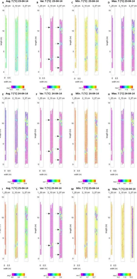
During 23-04-14, daily average streambed temperature ranged from 10.5 °C to 10.6 °C for flume 1_25 cm, from 10.4 °C to 10.6 °C for flume 2_10 cm, and from 10.3 °C to 10.6 °C for flume 3_07 cm (Figure 5 A), with a mean daily value along and across all flumes of 10.5±0.0
C.
Approximate location of Figure 5
where aquatic vegetation coverage was sparser and/or sediments were exposed. The warmest and most variable streambed temperatures across the 3-day study were observed on 24-04-14, a relatively warm, clear-sky day (Table 5). Average temperature values calculated for 24-04-14 and over space exhibited relatively high variability, ranging from 10.9 °C to 12.2 °C for flume 1_25 cm, from 10.5 °C to 12.9 °C for flume 2_10 cm, from 10.6 °C to 12.8 °C for flume 3_07 cm (Figure 5 E), with a daily mean value of 11.0±0.4 °C across and along all flumes. On 24-04-14, flume 3_07 cm was the one to exhibit the most extreme streambed temperature values; in fact, variance in flume 3_07 cm ranged from 0.0 to 24.0 °C (Figure 5 F) due to different warming and cooling gradients between vegetated vs. un-vegetated shallow water areas and bare exposed sediment features. The greatest response to increased global solar irradiation receipt for 24-04-14 for flume 3_07 cm resulted in a daily maximum streambed temperature registered that was 2.8 °C warmer than the maximum in flume 2_10 cm and 13.8 °C warmer than the maximum recorded in flume 1_25 cm (Figure 5 H). Similarly, minimum streambed temperatures for flume 3_07 cm exhibited a more intense night cooling compared to the deeper flumes: minimum streambed temperature values were in fact 0.4 °C and 3.1 °C colder than those of flume 1_25 cm and 2_10 cm, respectively (Figure 5 G). The lowest streambed temperatures coincided with heavy rain and colder air temperature on 25-04-14. The absolute lower limit of minimum streambed temperature ranges for the shallower flumes (2_10 and 3_07) was registered on 25-04-14 (Figure 5 M), while absolute maximum streambed temperature values for these flumes were approximately half of those recorded during clear-sky conditions (24-04-14) (Figure 5 N). In contrast, flume 1_25 cm was less responsive to the change in meteorological conditions compared to the shallower flumes. Absolute minimum streambed temperatures for flume 1_25 cm were higher on 25-04-14 than on 24-04-14 (10.2 °C and 9.9 °C respectively), whereas absolute maximum streambed temperatures did not vary substantially between 24-04-14 to 25-04-14 (13.3 and 13.2 °C respectively).
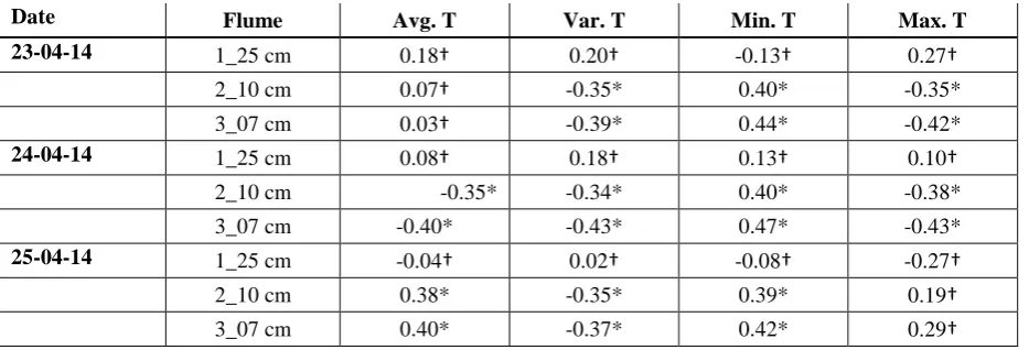
-0.43 and 0.29 for 23-04-14, 24-04-14 and 25-04-14, respectively). Correlation values for average streambed temperatures vs. water depths appeared to be less strong and less variable among flumes and dates than those for maximum and minimum streambed temperatures.
4. Discussion
This article reports the potential drought impacts on the thermal regime of lowland gravel-bed rivers. Continuous observations of temperature differences between surface water inflow and outflow and spatial patterns of streambed temperatures in three outdoor flumes characterized by different water depths and co-evolved vegetation coverage over three days (23/25-04-14) revealed complex thermal variability. The interaction between different water depths along the characteristic pool-riffle-pool sequences and different vegetation coverage created water depth gradients along and across the three flumes with the formation of a variety of complex hydrologic habitats.
Net radiation is generally the main component of total energy flux in river systems (Caissie, 2006), accounting for 56 % of the total heat gain and for 49 % of heat loss in the River Exe, U.K. (Webb and Zhang, 1997). In our systems, solar radiation was the main flux responsible for the daily outflow water temperature variations in the flumes (on average net radiation contributed for 64% to the total heat budget variations during the day and for 83% to the total heat loss during the night as simulated with our model). In addition, it has previously been acknowledged that the relationship between water and air temperature in a Devon river system is stronger and more sensitive for flows in the range below median discharge (Webb et al., 2003). Accordingly, in our study, the shallowest flume, 3_07 cm, representative of severe drought conditions, was especially responsive to fluctuations in solar radiation receipt and changes in air temperature. Using the high spatio-temporal capabilities of FO-DTS, it was possible to characterize the resulting high variability of thermal patterns in the flumes. Diverse meteorological conditions during the study period translated into different inter-flume streambed temperatures responses to radiation input, with inter-flume 1_25 cm being the least responsive and the shallower flumes instead showing greater spatial and temporal temperature heterogeneity at the water-sediment interface. Similarly, surface outflow temperature variations were more pronounced in the shallower flumes, as shallower water bodies are characterized by reduced thermal capacity and greater water temperature fluctuations (Clark et al., 1999).
exposed directly to solar radiation during daytime and were not sheltered from longwave radiation loss at night time, resulting in greater and quicker daytime warming compared to submerged areas, and faster night time cooling. A diel difference of 20.3 °C between the hottest (27.1 °C) and the coldest spot (6.8 °C) was registered for streambed temperatures for flume 3_07 cm on 24-04-14.
Special attention should be paid to maximum temperature as this is the most stressful for aquatic organisms, particularly under extreme meteorological conditions (e.g. droughts), when maximum values could be greater than their thermal tolerance threshold (Maazouzi et al., 2011). As reported by Dixon et al. (2009), most ectothermic organisms, representing 99.9% of species on Earth (Atkinson and Sibly, 1997), possess a similar thermal window situated around ~ 20 °C, a range within which the organisms’ development can occur. Ecological evidence, from the community to the individual level, showing a significant increase in the proportion of small-size species as a response mechanism to global warming (Daufresne et al., 2009) and to drought conditions (Ledger et al., 2011) has already been reported. In natural riverine ecosystems, obstacles (e.g. macrophytes aggregations) and streambed roughness (e.g. pool-riffle sequences) drive hydrological exchange processes between shallow groundwater and surface water through the hyporheic zone, due to discontinuities in slope and depth and changes in the direction of the flow (Brunke and Gonser, 1997). The direction of exchange processes varies with hydraulic head, whereas sediments permeability controls flow amount. The interactions between groundwater and surface water are characterized by a high temporal and spatial variability, due to seasonal fluctuations of surface water levels. Thus the resulting ecological impacts on riverine ecosystems vary seasonally (Krause and Bronstert, 2007). Under typical summer conditions of low flow base flow mainly originates from groundwater, with contributions up to 10% of the total river discharge (Krause and Bronstert, 2007). During hydrological stress conditions, these groundwater fluxes can act as an effective buffer against stream water warming because colder water is discharged to the stream when the stream most extreme temperatures are apt to occur (Poole and Berman, 2001). Hyporheic exchange promotes the formation of a mosaic of horizontal and vertical groundwater temperatures across the aquifer able to ameliorate particularly extreme stream maximum temperatures. Upwelling of colder groundwater into the main channel during low-flow conditions has ecological significance for biota, as it maintains minimum discharge able to support a diversified aquatic macrophytes community, it creates cold water refugia for stenotherms and for example it is essential for the survival of cold water fishes like salmonids (Ebersole et al., 2003). Under future climate change with stream maximum temperatures likely exceeding actual values, it is evident how hyporheic flow becomes increasingly strategic and essential in supporting healthy aquatic communities.
stream temperatures, especially on maximum temperatures during summer months (Story et al., 2003; Johnson, 2004; Danehy et al., 2005; Webb and Crisp, 2006; Hannah et al., 2008; Malcolm et al., 2008; Garner et al., 2014; Garner et al., 2015a). However, to our knowledge, ours is the first work exploring the combined effect of different water depths and co-evolved aquatic vegetation coverage on both surface and streambed temperature patterns at high spatial and temporal resolution. When assessing the effect of shading on stream water, the type of vegetation (e.g. growth form and morphology) and its density is an important element to be considered (Lövstedt and Bengtsson, 2008). During a clear day in presence of large stand of submerged macrophytes in a shallow water body, Dale and Gillespie (1977b) found that little light energy reached the streambed. Temperatures were higher at the water surface and lower at the water-streambed interface, resulting in a steep vertical temperature gradient in the water column; with sparse vegetation, smaller differences between surface water and streambed developed. Similarly, Clark et al. (1999) recorded vertical temperature contrasts due to the isolation from the main flow of a thin surface layer by aquatic vegetation such as Ranunculus spp.; this layer was subjected to strong heating by the sun (up to 2.7 °C above surface temperature in non-vegetated water areas), whereas the flow below the floating vegetation was protected. Furthermore, the temperature near the bottom of shallow water bodies where no shadows were cast by macrophytes varied with incoming solar radiation and quick temperature fluctuations were observed when radiation changed (up to + 10 °C in 6 hours at 0.20 cm depth when average net radiation was ~ 500 W/m2; Dale and Gillespie, 1977a). In our study, we observed that streambed temperature extrema in flume 1_25 were generally lower than surface water values measured at the flume outlet. Streambed minimum temperatures were consistently lower than minimum surface water values throughout the duration of the experiment and maximum streambed temperatures were lower on 23-04-14 and 24-04-14. These findings are therefore likely due to the combination of deeper water and higher vegetation coverage relative to the other flumes, which increased the water body thermal capacity and buffered daytime atmospheric energy receipt, respectively. In contrast, this pattern was absent for the shallower flumes having greater exposed sediment:water surface ratios (leading to lower thermal buffering capacities) and more patchy shading by the sparser vegetation. In this experiment, however, it was difficult to separate the single impacts of different vegetation coverage from different water depths on flumes thermal regimes, and rather the combined effects were observed. More research on the subject needs to be carried out to evaluate the influence of each factor.
in particular, minimum streambed temperatures exhibited a faster and greater night-time cooling compared to the deeper flumes, with minimum streambed temperatures (6.7 °C) almost attaining minimum air temperature on 25-04-14 (6.9 °C). In contrast, in the deepest flume, the combined effect of the greater thermal capacity and the lower heat losses (potentially due to reduced evaporation in comparison to non-vegetated sections; Dale and Gillespie, 1976), prevented large daily temperature differences between minimum and maximum values. The more homogenous and dense vegetation coverage and the fact that all sediments were saturated translated into a less diversified spatial and temporal streambed temperature patterns distribution, with smaller differences between extreme temperature values both in space (along the flume) and in time (between day/night time and between different dates). Given the reasonable degree of correlation between vegetation coverage and water depth (section 3.2) and water depth and streambed temperature metrics (section 3.4), this result supported our initial hypothesis that the combined effects of shallower water depth and sparser vegetation coverage would drive more marked temperature patterns in shallower flumes.
5. Conclusions
Using the high spatio-temporal capabilities of FO-DTS, we were able to detect high variability of thermal dynamics in co-evolved vegetated flumes with varying water depths. Our results indicate that variations in water depth, co-evolved aquatic vegetation coverage and morphologic features (pool-riffle-pool sequences) were major determinants in creating a complex spatial heterogeneity within the 15-m long and 0.5-m wide artificial channels. First, shallower water areas in the flumes, characterized by lower thermal capacity than the deeper areas, showed greater fluctuations in temperatures, with the exposed sediment features (riffle sections) distinctly showing the most extreme temperature values due to the lower heat capacity compared to the one of the water areas. Second, vegetation coverage likely also played a fundamental role via shading. Dense and continuous vegetation coverage, like that found in flume 1_25 cm, prohibited solar radiation from directly impacting the streambed sediments and reduced the evaporation rate from the flumes. Finally, water levels, together with vegetation, controlled the sensitivity of the flume temperature regimes to different meteorological conditions, particularly to changes in air temperature and solar radiation receipt. Given the expectation of more frequent and intense drought conditions under projected climate change, despite the use of artificial channels, our results highlight the importance of maintaining minimum water level conditions in lowland streams that are able to host a stable aquatic vegetation community. Minimum water levels, together with the aquatic vegetation community, could promote the formation of complex thermal and hydrological habitats, able to better buffer the negative effects of extreme events such as heat waves.
terrestrialization occurring in lowland lotic ecosystems, and of its effects on river temperature regimes. Even though it is irrefutable that different growth forms possess different shading abilities, the consequences of increased numbers of riparian/invasive species replacing strictly aquatic plants (as projected under more severe future drought scenarios) to both surface and streambed temperatures is still unknown. Furthermore, extreme water temperatures during drought conditions which could exceed ectothermic organisms’ upper limit thermal tolerance, stress the importance of the availability of both thermal and hydrological refugia (e.g. the hyporheic zone) to increase invertebrates and fish population resistance during drying events and resilience after the disturbance. The effects of water level fluctuations not only could imply different thermal dynamics in space and time but, on a long term, could alter ecosystem functioning and biodiversity as well, with riparian/invasive species replacing strictly aquatic plants, and with ectothermic organisms resistance/resilience threated by the altered thermal regimes whether some effective protection processes for in-stream biota are not occurring (e.g. due to disrupted surface-groundwater linkages).
Acknowledgements
The authors wish to thank the DRI-STREAM mesocosms facility and Fobdown Watercress Farm for the use of their facilities, and the entire Leverhulme Hyporheic Zone Network Team for their support and insight. Financial support for the experiment was provided by The Leverhulme Trust through the project ‘‘Where rivers, groundwater and disciplines meet: A
References
Arrigoni AS, Poole GC, Mertes LAK, O' Daniel SJ, Woessner WW, Thomas SA. 2008. Buffered, lagged, or cooled? Disentangling hyporheic influences on temperature cycles in stream channels. Water Resources Research 44, W09418.
Atkinson D, Sibly RM. 1997. Why are organisms usually bigger in colder environments? Making sense of a life history puzzle. Trends in Ecology & Evolution 12: 235-239.
Bates BC, Kundzewicz ZW, Wu S, Palutikof JP. 2008. Climate Change and Water. Technical Paper of the Intergovernmental Panel on Climate Change: 210 pp.
Bengtsson H. 2015. MatrixStats: Functions that Apply to Rows and Columns of Matrices (and to Vectors). R package version 0.50.1., doi:http://CRAN.R-project.org/package=matrixStats.
Berman R, Brown T. 1986. Heat capacity of minerals in the system Na2O-K2O-CaO-MgO-FeO-Fe2O3-Al2O3-SiO2-TiO2-H2O-CO2: representation, estimation, and high temperature extrapolation. Contributions to Mineralogy and Petrology 94: 262-262.
Bogan MT, Boersma KS, Lytle DA. 2015. Resistance and resilience of invertebrate communities to seasonal and supraseasonal drought in arid-land headwater streams. Freshwater Biology 60: 2547-2558.
Bogan T, Mohseni O, Stefan HG. 2003. Stream temperature-equilibrium temperature relationship. Water Resources Research 39: 1245.
Bond N, Lake P, Arthington A. 2008. The impacts of drought on freshwater ecosystems: an Australian perspective. Hydrobiologia 600: 3-16.
Bornette G, Puijalon S. 2011. Response of aquatic plants to abiotic factors: a review. Aquatic Sciences 73: 1-14.
Boulton A. 2003. Parallels and contrasts in the effects of drought on stream macroinvertebrate assemblages. Freshwater Biology 48: 1173-1185.
Boyd M, Kasper B. 2003. Analytical methods for dynamic open channel heat and mass transfer: methodology for Heat Source Model Version 7.0, Watershed Sciences Inc., Portland, OR, USA, found at: http://www.deq.state.or.us/wq/TMDLs/tools.htm.
Briggs MA, Lautz LK, McKenzie JM, Gordon RP, Hare DK. 2012. Using high-resolution distributed temperature sensing to quantify spatial and temporal variability in vertical hyporheic flux, Water Resources Research 48: 1-16.
Brunke M, Gonser T. 1997. The ecological significance of exchange processes between rivers and groundwater.Freshwater Biology37: 1-33.
Caissie D. 2006. The thermal regime of rivers: a review. Freshwater Biology 51: 1389-1406.
Clark E, Webb B, Ladle M. 1999. Microthermal gradients and ecological implications in Dorset rivers. Hydrological Processes 13: 423-438.
Constantz J. 1998. Interaction between stream temperature, streamflow, and groundwater exchanges in alpine streams. Water Resources Research 34: 1609-1615.
Dale HM, Gillespie T. 1976. The influence of floating vascular plants on the diurnal fluctuations of temperature near the water surface in early spring. Hydrobiologia 49: 245-256.
Dale HM, Gillespie T. 1977a. Diurnal fluctuations of temperature near the bottom of shallow water bodies as affected by solar radiation, bottom colour and water circulation. Hydrobiologia 55: 87-92.
Dale HM, Gillespie TJ. 1977b. The influence of submersed aquatic plants on temperature gradient in shallow water bodies. Canadian Journal of Botany 55: 2216-2225.
Dallas H, Rivers-Moore N. 2011. Micro-scale heterogeneity in water temperature. Water SA 37: 505-505.
Danehy RJ, Colson CG, Parrett KB, Duke SD. 2005. Patterns and sources of thermal heterogeneity in small mountain streams within a forested setting. Forest Ecology and Management 208: 287-302.
Daufresne M, Lengfellner K, Sommer U. 2009. Global warming benefits the small in aquatic ecosystems. Proceedings Of The National Academy Of Sciences Of The United States Of America 106: 12788-12793.
Dixon AFG, Hon k A, Keil P, Kotela MAA, Šizling AL, Jarošík V. 2009. Relationship
between the minimum and maximum temperature thresholds for development in insects. Functional Ecology 23: 257-264.
Döll P, Zhang J. 2010. Impact of climate change on freshwater ecosystems: a global-scale analysis of ecologically relevant river flow alterations. Hydrology and Earth System Sciences 14: 783-799.
Easterling D, Evans J, Groisman P, Karl T, Kunkel K, Ambenje P. 2000. Observed variability and trends in extreme climate events: A brief review. Bulletin of the American Meteorological Society 81: 417-425.
Ebersole JL, Liss WJ, Frissell CA. 2003. Cold water patches in warm streams: physicochemical characteristics and the influence of shading. JAWRA Journal of the
American Water Resources Association39: 355-368. ESRI. 2011. ArcGIS Desktop: Release 10.
Franklin P, Dunbar M, Whitehead P. 2008. Flow controls on lowland river macrophytes: A review. Science of the Total Environment 400: 369-378.
Fullerton AH, Torgersen CE, Lawler JJ, Faux RN, Steel EA, Beechie TJ, Ebersole JL, Leibowitz SG. 2015. Rethinking the longitudinal stream temperature paradigm: region-wide comparison of thermal infrared imagery reveals unexpected complexity of river temperatures. Hydrological Processes 29: 4719-4737.
Garner G, Malcolm IA, Sadler JP, Hannah DM. 2014. What causes cooling water temperature gradients in a forested stream reach? Hydrology and Earth System Sciences 18: 5361-5376.
Garner G, Malcolm IA, Sadler JP, Millar CP, Hannah DM. 2015a. Inter-annual variability in the effects of riparian woodland on micro-climate, energy exchanges and water temperature of an upland Scottish stream. Hydrological Processes 29: 1080-1095.
Garner G, Van Loon AF, Prudhomme C, Hannah DM. 2015b. Hydroclimatology of extreme river flows. Freshwater Biology 60: 2461-2476.
Giller PS, Malmqvist B. 1998. The biology of streams and rivers. Oxford University Press: Oxford.
Green JC. 2005. Modelling flow resistance in vegetated streams: Review and development of new theory.Hydrological Processes19: 1245-1259.
Grime JP. 1979. Plant strategies and vegetation processes. John Wiley: Chichester.
Hannah DM, Garner G. 2015. River water temperature in the United Kingdom: Changes over the 20th century and possible changes over the 21st century.Progress in Physical Geography 38: 68-92.
Hannah DM, Malcolm IA, Soulsby C, Youngson AF. 2008. A comparison of forest and moorland stream microclimate, heat exchanges and thermal dynamics. Hydrological Processes 22: 919-940.
Hannah DM, Malcolm IA, Soulsby C, Youngson AF. 2004. Heat exchanges and temperatures within a salmon spawning stream in the Cairngorms, Scotland: seasonal and sub-seasonal dynamics. River Research and Applications 20: 635-652.
Hausner MB, Suárez F, Glander KE, van dG, Selker JS, Tyler SW. 2011. Calibrating single-ended fiber-optic Raman spectra distributed temperature sensing data. Sensors 11: 10859-10879.
Hester E, Doyle M, Poole G. 2009. The influence of in-stream structures on summer water temperatures via induced hyporheic exchange. Limnology and Oceanography 54: 355-367.
Jentsch A, Kreyling J, Beierkuhnlein C. 2007. A new generation of climate change experiments: events, not trends. Frontiers in Ecology and the Environment 5: 315–324.
Johnson MF, Wilby RL. 2013. Shield or not to shield: Effects of solar radiation on water temperature sensor accuracy. Water 5: 1622-1637.
Johnson SL. 2004. Factors influencing stream temperatures in small streams: Substrate effects and a shading experiment. Canadian Journal of Fisheries and Aquatic Sciences 61: 913-923.
Krause S, Blume T. 2013. Impact of seasonal variability and monitoring mode on the adequacy of fiber-optic distributed temperature sensing at aquifer-river interfaces. Water Resources Research 49: 2408-2423.
Krause S, Bronstert A. 2007. The impact of groundwater–surface water interactions on the water balance of a mesoscale lowland river catchment in northeastern Germany. Hydrological Processes 21: 169-184.
Krause S, Taylor SL, Weatherill J, Haffenden A, Levy A, Cassidy NJ, Thomas PA. 2012. Fibre-optic distributed temperature sensing for characterizing the impacts of vegetation coverage on thermal patterns in woodlands. Ecohydrology 6: 754-764.
Laizé C,L.R., Acreman MC, Schneider C, Dunbar MJ, Houghton-Carr H, Flörke M, Hannah DM. 2014. Projected flow alteration and ecological risk for pan-European rivers. River Research and Applications 30: 299-314.
Lake PS. 2003. Ecological effects of perturbation by drought in flowing waters. Freshwater Biology 48: 1161-1172.
Ledger ME, Edwards FK, Brown LE, Milner A, Woodward G. 2011. Impact of simulated drought on ecosystem biomass production: an experimental test in stream mesocosms. Global Change Biology 17: 2288-2297.
Ledger ME, Milner AM. 2015. Extreme events in running waters. Freshwater Biology 60: 2455-2460.
Leigh C, Bush A, Harrison ET, Ho SS, Luke L, Rolls RJ, Ledger ME. 2015. Ecological effects of extreme climatic events on riverine ecosystems: insights from Australia. Freshwater Biology 60: 2620-2638.
Lövstedt CB, Bengtsson L. 2008. Density-driven current between reed belts and open water in a shallow lake. Water Resources Research 44, W10413.
Malcolm IA, Soulsby C, Hannah D, Bacon PJ, Youngsen AF, Tetzlaff D. 2008. The influence of riparian woodland on stream temperatures: implications for the performance of juvenile salmonids. Hydrological Processes 22: 968-979.
Matthews WJ. 1998. Patterns in Freshwater Fish Ecology. Chapman and Hall: London.
Mebane CA, Maret TR, Simon NS. 2014. Linking nutrient enrichment and streamflow to macrophytes in agricultural streams. Hydrobiologia 722: 143-158.
Met Office. 2006. UK Daily Temperature Data, Part of the Met Office Integrated Data Archive System (MIDAS). NCAS British Atmospheric Data Centre, 15/12/2016.
http://catalogue.ceda.ac.uk/uuid/1bb479d3b1e38c339adb9c82c15579d8.
Mosley MP, Zimpfer GL. 1978. Hardware models in geomorphology.Progress in Physical Geography 2: 438-461.
Palmer M, Lettenmaier D, Poff N, Postel S, Richter B, Warner R. 2009. Climate Change and River Ecosystems: Protection and Adaptation Options. Environmental management 44: 1053-1068.
Poff NL, Zimmerman JKH. 2010. Ecological responses to altered flow regimes: a literature review to inform the science and management of environmental flows. Freshwater Biology 55: 194-205.
Poole GC, Berman CH. 2001. An ecological perspective on in-stream temperature: natural heat dynamics and mechanisms of human-caused thermal degradation. Environmental Management 27: 787-802.
Poynter AJW. 2014. Impacts of environmental stressors on the River Itchen Ranunculus community. PhD dissertation, School of Geography, Earth and Environmental Sciences, University of Birmingham U.K.
R Core Team. 2013. R: A language and environment for statistical computing. R Foundation for Statistical Computing. ISBN 3-900051-07-0, URL http://www.R-project.org/.
Richards KS. 1976. The morphology of riffle-pool sequences.Earth Surface Processes1(1):
71-88.
Riis T, Biggs BJF. 2003. Hydrologic and hydraulic control of macrophyte establishment and performance in streams. Limnology and Oceanography 48: 1488-1497.
Riis T, Biggs BF. 2001. Distribution of macrophytes in New Zealand streams and lakes in relation to disturbance frequency and resource supply-a synthesis and conceptual model. New Zealand Journal of Marine and Freshwater Research 35: 255-267.
Riis T, Suren AM, Clausen B, Sand Jensen K. 2008. Vegetation and flow regime in lowland streams. Freshwater Biology 53: 1531-1543.
Schuyler AE. 1984. Classification of life forms and growth forms of aquatic macrophytes. Bartonia 50: 8-11.
Sebok E, Duque C, Engesgaard P, Boegh E. 2015. Application of Distributed Temperature Sensing for coupled mapping of sedimentation processes and spatio-temporal variability of groundwater discharge in soft-bedded streams. Hydrological Processes 29: 3408-3422.
Selker JS, Thévenaz L, Huwald H, Mallet A, Luxemburg W, Giesen VD, Stejskal M, Zeman J, Westhoff M, Parlange MB. 2006a. Distributed fiber optic temperature sensing for hydrologic systems. Water Resources Research 42, W12202.
Selker JS, Giesen VD, Westhoff M, Luxemburg W, Parlange MB. 2006b. Fiber optics opens window on stream dynamics. Geophysical Research Letters 33: L24401.
Sinokrot BA, Stefan HG. 1993. Stream temperature dynamics: measurements and modeling. Water Resources Research 29: 2299-2312.
Story A, Moore RD, Macdonald JS. 2003. Stream temperatures in two shaded reaches below cutblocks and logging roads: downstream cooling linked to subsurface hydrology. Canadian Journal of Forest Research 33: 1383-1396.
Stromberg JC, Bagstad KJ, Leenhouts JM, Lite SJ, Makings E. 2005. Effects of stream flow intermittency on riparian vegetation of a semiarid region river (San Pedro River, Arizona). River Research and Applications 21: 925-938.
Thomaz SM, Cunha ERD. 2010. The role of macrophytes in habitat structuring in aquatic ecosystems: methods of measurement, causes and consequences on animal assemblages' composition and biodiversity. Acta Limnologica Brasiliensia 22: 218-236.
Tyler SW, Selker JS, Hausner MB, Hatch CE, Torgersen T, Thodal CE, Schladow SG. 2009. Environmental temperature sensing using Raman spectra DTS fiber-optic methods. Water Resources Research 45, W00D23.
van de Giesen NC, Steele Dunne S, Jansen J, Hoes O, Hausner M, Tyler S, Selker J. 2012. Double-ended calibration of fiber-optic Raman spectra distributed temperature sensing data. Sensors 12: 5471-5485.
Vörösmarty CJ, Mcintyre PB, Gessner MO, Dudgeon D, Prusevich A, Green P, Glidden S, Bunn SE, Sullivan CA, Reidy Liermann C, Davies PM. 2010. Global threats to human water security and river biodiversity. Nature 467: 555-561.
Warfe D, Barmuta L. 2006. Habitat structural complexity mediates food web dynamics in a freshwater macrophyte community. Oecologia 150: 141-154.
Webb BW, Clack PD, Walling DE. 2003. Water-air temperature relationships in a Devon river system and the role of flow. Hydrological Processes 17: 3069-3084.
Webb BW, Hannah D, Moore RD, Brown LE, Nobilis F. 2008. Recent advances in stream and river temperature research. Hydrological Processes 22: 902-918.
Webb BW, Zhang Y. 1997. Spatial and seasonal variability in the components of the river heat budget. Hydrological Processes 11: 79-101.
Webb BW. 1996. Trends in stream and river temperature. Hydrological Processes 10: 205-226.
Westwood CG, Teeuw RM, Wade PM, Holmes NTH, Guyard P. 2006. Influences of environmental conditions on macrophyte communities in drought-affected headwater streams. River Research and Applications 22: 703-726.
Figure 2. Temperature (°C) and precipitation (mm) at the site over the duration of the experiment
[image:26.595.77.528.157.463.2]Figure 3. Spatial distribution of A) sediments thickness (cm), B) water depth (cm) and C) vegetation
Figure 4. Surface water temperature measured at the inflow in flume 2_10 cm and at the outflow of
Figure 5. Average (A), variance (B), minimum (C) and maximum (D) spatial streambed temperature
Table 1. Particle size distribution in flume sediments.
Table 2. FO-DTS coverage of flume surfaces: number of FO-cable transects per flume, max length per cable transect per flume (m) and discarded points per transect per flume (*For 1_25 cm FO-cable transects started 1 m
downstream).
Flume DTS cable transect DTS cable transect
length (m) Points discarded
1_25 cm 2 13.7* 8+5
2_10 cm 4 13.5 11+13+8+5
[image:30.595.70.485.385.529.2]3_07 cm 4 12.7 0+2+6+3
Table 3. Flume average sediment thickness (cm) and volume of sediment (m3), average water depth (cm), pool water depth (cm), discharge (x 10-4 m3/s), velocity (x 10-2 m/s) and volume of surface water (m3), proportion of sediment surface exposed to the air (m2) with relative percentage to total flume area (%).
Flume Sediment thickness (cm) Volume of sediment
(m3)
Water depth (cm) Pool water depth (cm) Discharge (x 10-4 m3/s)
Velocity (x 10-2
m/s)
Volume of surface
water (m3)
Area of exposed sediment
(m2)
1_25
cm 17.6 1.3 23.4 27.2 13.00 1.11 1.7
0.00 (0.0%)
2_10
cm 18.6 1.4 7.1 11.1 4.77 1.37 0.5
0.05 (0.7%)
3_07
cm 17.8 1.3 3.4 6.1 0.38 0.22 0.3
0.51 (7.2%)
Particle size (mm) Percentage (%)
< 0.35 2
0.35 - 2 6
2 - 11 12
Table 4. Daily averages for air temperature (°C), global solar irradiation (KJ/m2 d), flume average outflow surface water temperatures with standard deviation and range values (minimum-maximum) for 23-04-14, 24-04-14 and 25-04-14 (*Data taken from Southampton meteorological station, about 30 km distance).
Day Air T
(°C)
Global solar irradiation (KJ/ m2 d)*
T 1_25 cm out (°C)
T 2_10 cm out (°C)
T 3_07 cm out (°C)
23-04-2014 10.2 8280 10.5±0.1 (10.4-10.6) 10.5±0.1 (10.4-10.6) 10.5±0.1 (10.4-10.9)
24-04-2014 10.9 19640 10.7±0.5 (10.3-11.8) 10.7±0.4 (10.3-11.6) 11.1±1.1 (10.1-13.5)
[image:31.595.79.518.115.198.2]Table 5. Mean with standard deviation and range values for average, variance, minimum and maximum streambed temperature patterns for each flume during the experiment.
Date Flume
Avg. T (°C) Var. T (°C) Min. T (°C) Max. T (°C)
Mean Range Mean Range Mean Range Mean Range
23-04-14 1_25 cm 10.5±0.0
10.5-10.6
0.0±0.0 0.0-0.0 10.2±0.0 10.0-10.3
10.9±0.1 10.8-11.1 2_10 cm 10.5±0.0
10.4-10.6
0.0±0.1 0.0-0.4 10.1±0.1 9.4-10.2
11.0±0.2 10.7-12.0 3_07 cm 10.5±0.0
10.3-10.6
0.1±0.1 0.0-0.7 10.0±0.2 9.3-10.3
11.2±0.4 10.7-12.9
24-04-14 1_25 cm 11.0±0.1
10.9-11.2
0.3±0.1 0.1-0.8 10.1±0.1 9.9-10.2
12.2±0.4 11.6-13.3 2_10 cm 11.0±0.4
10.5-12.9
1.2±2.9 0.0-19.4
9.9±0.5 7.1-10.2
13.0±2.3 11.0-24.3 3_07 cm 11.0±0.5
10.6-12.8
2.8±5.1 0.0-24.0
9.5±0.9 6.8-10.3
14.4±3.9 11.2-27.1
25-04-14 1_25 cm 11.0±0.0
10.9-11.1
0.1±0.0 0.0-0.1 10.6±0.1 10.2-10.7
13.0±0.1 12.8-13.2 2_10 cm 10.6±0.3
9.0-11.1
0.1±0.1 0.0-0.8 10.1±0.6 7.1-10.7
12.8±0.2 12.4-13.3 3_07 cm 10.2±0.4
8.8-10.6
0.1±0.2 0.0-0.8 9.5±0.9 6.7-10.2
Table 6. Spatial correlation analysis results for 23-04-14, 24-04-14, 25-04-14 obtained for the correlation of average, variance, minimum and maximum streambed temperatures in each flume vs. correspondent water level values (* p-value < 0.001; no significant p-p-value).
Date Flume Avg. T Var. T Min. T Max. T
23-04-14 1_25 cm 0.18 0.20 -0.13 0.27
2_10 cm 0.07 -0.35* 0.40* -0.35*
3_07 cm 0.03 -0.39* 0.44* -0.42*
24-04-14 1_25 cm 0.08 0.18 0.13 0.10
2_10 cm -0.35* -0.34* 0.40* -0.38*
3_07 cm -0.40* -0.43* 0.47* -0.43*
25-04-14 1_25 cm -0.04 0.02 -0.08 -0.27
2_10 cm 0.38* -0.35* 0.39* 0.19