White Rose Research Online URL for this paper:
http://eprints.whiterose.ac.uk/114592/
Version: Accepted Version
Article:
Dong, Y.-Y., Dong, C.-X., Liu, W. et al. (2 more authors) (2017) 2-D DOA Estimation for
L-Shaped Array With Array Aperture and Snapshots Extension Techniques. IEEE Signal
Processing Letters, 24 (4). pp. 495-499. ISSN 1070-9908
https://doi.org/10.1109/LSP.2017.2676124
© 2017 IEEE. Personal use of this material is permitted. Permission from IEEE must be
obtained for all other users, including reprinting/ republishing this material for advertising or
promotional purposes, creating new collective works for resale or redistribution to servers
or lists, or reuse of any copyrighted components of this work in other works. Reproduced
in accordance with the publisher's self-archiving policy.
[email protected] https://eprints.whiterose.ac.uk/
Reuse
Items deposited in White Rose Research Online are protected by copyright, with all rights reserved unless indicated otherwise. They may be downloaded and/or printed for private study, or other acts as permitted by national copyright laws. The publisher or other rights holders may allow further reproduction and re-use of the full text version. This is indicated by the licence information on the White Rose Research Online record for the item.
Takedown
If you consider content in White Rose Research Online to be in breach of UK law, please notify us by
2-D DOA Estimation for L-shaped Array with
Array Aperture and Snapshots Extension Techniques
Yang-Yang Dong, Chun-xi Dong, Wei Liu,
Senior Member, IEEE
, Hua Chen, and Guo-qing Zhao
Abstract—A two dimensional (2-D) direction of arrival (DOA) estimation method for L-shaped array with automatic pairing is proposed. It exploits the conjugate symmetry property of the ar-ray manifold matrix to increase the effective arar-ray aperture and the number of virtual snapshots simultaneously, and then applies the principle of MUSIC to construct an angle cost function and transforms the conventional 2-D search into 1-D via a Rayleigh quotient, which can greatly reduce the computation complexity. Finally, the azimuth and elevation angles are estimated without pair matching. Simulation results show that the proposed method has a better performance and can resolve more sources than some existing computationally efficient methods.
Index Terms—two dimensional, direction of arrival estimation, L-shaped array, Rayleigh quotient, pair matching.
I. INTRODUCTION
T
WO dimensional (2-D) direction of arrival (DOA) estima-tion is a basic problem in array signal processing and has wide applications in wireless communications, radar, sonar, etc [1]. For 2-D DOA estimation, many geometrical structures have been developed, such as L-shaped array, circular array, parallel linear arrays, rectangular array, etc [1]–[11]. In partic-ular, due to its simplicity and effectiveness, the L-shaped array has attracted a lot of attention in the past, based on which many computationally efficient algorithms have been proposed [12]– [25]. These algorithms can be divided into two classes. One is to estimate the angles corresponding to each uniform linear subarray via applying 1-D DOA estimation algorithms to the received data or reconstructed data of each subarray [12], [13], [18]–[22], [25]. However, additional angle pairing is needed, which may not work for some special cases and affect the overall performance [14]. To avoid this problem, the second class of algorithms can pair the angles automatically, such as the joint SVD [14], parallel factor analysis [15], and the effective array aperture extension method [23].However, neither of them works when the number of sources is larger than the number of elements of each uniform linear subarray: to estimate angles ofKsources, the total number of Copyright (c) 2017 IEEE. Personal use of this material is permitted. However, permission to use this material for any other purposes must be obtained from the IEEE by sending a request to [email protected]. This work was supported by the National High-tech R&D Program of China (863 Program) under Grants 2015AA80XXX86H.
Y.-Y. Dong, C.-x. Dong, and G.-q. Zhao are with the Key Laboratory of Electronic Information Countermeasure and Simulation Technology, Ministry of Education, Xidian University, Xi’an 710071, China ([email protected]; [email protected]; [email protected]).
W. Liu is with the Department of Electronic and Electrical Engineering, University of Sheffield, S1 4ET, U.K. ([email protected]).
H. Chen is with the School of Electronic Information Engineering, Tianjin University, Tianjin 300072, China ([email protected]).
array elements of the L-shaped array Mtotal should satisfy
Mtotal > 2K. Although the maximum identifiable source number of the maximum likelihood (ML) method [11] and the 2D-MUSIC method [26] can overcome this limit, they require multidimensional spectrum peak search, which are too high in computational cost for many real-time applications.
In this work, we aim to increase the maximum number of resolvable sources with automatic pairing for L-shaped arrays, while avoiding the multi-dimensional search. First, by utilizing the conjugate symmetry property of the uniform linear array (ULA) manifold matrix, a large array-received-data-like (LARDL) matrix is constructed, which is similar to the way followed in [23]; however, different from [23], we also increase the number of virtual snapshots of the LARDL matrix, which is crucial to increase the maximum number of resolvable sources; then, we apply the 2-D MUSIC principle and obtain an unconstrained 2-D optimization problem. To solve the problem without 2-D search, we transform it to a Rayleigh quotient form by adding a constraint. Finally, the azimuth angles are estimated with 1-D search and the elevation angles are estimated via the special structure of the resultant eigenvectors. Simulation results show that the proposed method yields better results than the classic JSVD [14], PARAFAC [15], CODE [18], CESA [20], EAET [23], and AAEA [25]. Furthermore, the maximum number of iden-tifiable sources by the proposed method isMtotal−2.
Notations: Matrices and vectors are denoted by boldfaced capital letters and lower-case letters, respectively. (·)∗
, (·)T, and(·)H stand for conjugate, transpose, and conjugate trans-pose, respectively. E{·}, ⊗, ID, JD, 0m×n, diag{·}, and angle(·)denote the statistical expectation, Kronecker product, aD×D identity matrix, aD×Dexchange matrix with ones on its antidiagonal and zeros elsewhere, anm×nzero matrix, diagonalization and phase angle operator for complex number, respectively. D(:, p: q) represents a submatrix consisting of thepth to theqth columns of matrix D.
II. SIGNALMODEL
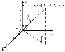
As shown in Fig.1, an L-shaped array consists of two orthogonalM-element uniform linear arrays with inter-sensor spacingdalongxandzaxes, respectively.Knarrowband far-field uncorrelated signals{sk(n)}Kk=1(n= 1,· · · , N,N is the
number of snapshots ) of wavelengthλimpinge from distinct directions with azimuth and elevation angles {(θk, φk)}Kk=1
x
y 1
2
M
1 2
M
k
k
( ), 1, 2, ,
k
[image:3.612.119.228.57.145.2]s n k K
Fig. 1. L-shaped array configuration for 2-D DOA estimation.
manifold matrices ofxandz subarrays as
Ax(θ)= [ax(θ1),ax(θ2),· · ·,ax(θK)], (1)
Az(φ)= [az(φ1),az(φ2),· · ·,az(φK)], (2) where
ax(θk)=[ax,1(θk), ax,2(θk),· · · , ax,M(θk)]T =[ej2πcosθkd/λ
,· · ·, ej2πMcosθkd/λ
]T,
az(φk)=[az,1(φk), az,2(φk),· · ·, az,M(φk)]T =[1, ej2πcosφkd/λ,· · ·, ej2π(M−1) cosφkd/λ]T.
Hence, the received signal ofxandz subarrays at thenth snapshot x(n)andz(n)can be represented by
x(n)=Ax(θ)s(n) +wx(n), (3)
z(n)=Az(φ)s(n) +wz(n), (4) where x(n) = [x1(n),· · · , xM(n)]T, z(n) = [z1(n), · · · , zM(n)]T, s(n) = [s1(n),· · ·, sK(n)]T represents the source signal vector, and wx(n) = [wx,1(n),· · ·, wx,M(n)]T and wz(n) = [wz,1(n),· · ·, wz,M(n)]T denote the additive noise vectors corresponding to thexandz subarrays, respec-tively. Similar to [23], it is assumed that the additive noises are temporally and spatially white with zero-mean and variance
σ2
w, and are uncorrelated with the incident signals.
III. PROPOSEDMETHOD
A. Array Aperture and Snapshots Extension
According to [23], [27], [28], the manifold matrix for an
M-element ULA is a Vandermonde matrix and possesses the conjugate symmetry property, i.e.,
JM(Ax(θ))∗=Ax(θ)Φ˜xr(θ), (5)
JM(Az(φ))∗=Az(φ)Φ˜zr(φ), (6) where
˜
Φxr(θ)=diag{e−j2π(M−1) cosθ1d/λ,
· · ·, e−j2π(M−1) cosθKd/λ },
˜
Φzr(φ)=diag{e−j2π(M−1) cosφ1d/λ,
· · ·, e−j2π(M−1) cosφKd/λ }.
We can see that the effective array aperture of a ULA can be increased via the conjugate operation. This is an effective technique and can improve the estimation performance signif-icantly [23].
However, although the EAET method in [23] only increases the array aperture, the number of virtual snapshots in the
LARDL matrix (viz. Eq.(16) in [23]) remainsM −1, which limits the maximum number of resolvable sources Kmax to
Kmax ≤ (M −1). To increase the array aperture and the virtual snapshots simultaneously, we first construct the cross-correlation matrixRxz as follows,
Rxz=E{x(n)zH(n)}=Ax(θ)RssAHz(φ), (7) where Rss = diag{p1,· · · , pK} and {pk}Kk=1 represent the
signal power set. With the assumptions made in Section II, this procedure can also reduce the effect of noise.
Similar to [14] and [23],Rxz can be divided into twoM× (M−1) matrices as follows,
Y1=Rxz(:,1 :M −1) =Ax(θ)RssAHz1(φ), (8) Y2=Rxz(:,2 :M) =Ax(θ)RssAHz2(φ), (9)
where Az1(φ) and Az2(φ) stand for the first and the last
(M − 1) rows of Az(φ), Az2(φ) = Az1(φ)Φz(φ) and
Φz(φ) = diag{ej2πcosφ1d/λ,· · · , ej2πcosφKd/λ}.
Considering (5) and using (8)-(9), we can construct a new LARDL matrix as follows,
Y=
Y1,JMY∗2 Y2,JMY∗1
=Ag(θ,φ)Sg(θ,φ), (10) where
Ag(θ,φ) =
h
ATx(θ),(Ax(θ)Φ∗z(φ)) TiT
,
Sg(θ,φ) =
h
RssAHz1(φ),Φz(φ)Φ˜xr(θ)RssATz1(φ)
i
.
In this way, both the array aperture and the number of virtual snapshots have been increased.
Note that the PM-ESPRIT method in [23] cannot be used for (10), as it requires two(M−1)array data sets to construct the matrix consisting of the azimuth rotation invariance factor. However, both the 2-D MUSIC and ML method can be applied to (10) to obtain 2-D DOA estimations with a multi-dimensional search. Next, we develop a novel estimation method to avoid the multidimensional search.
Remark 1: The dimensions ofAg(θ,φ)andSg(θ,φ)are 2M ×K and K×2(M −1), respectively, which results in the case that the number of array elements is larger than the number of snapshots. According to the subspace theory, the maximum number of identifiable sources cannot exceed max{2M−1,2(M−1)}, i.e.,2(M −1).
B. 2-D DOA Estimation Based on Rayleigh Quotient
Applying eigenvalue decomposition (EVD) to Ryy =
YYH, we have
Ryy =UsΛsUHs +UwΛwUHw, (11)
where Us and Uw represent the signal subspace and the noise subspace, respectively.1 We can minimize the following cost function with 2-D search and obtain the angle estimation results, i.e.,
{(ˆθk,φˆk)}Kk=1= arg min
θ,φ f(θ, φ), (12)
1For the non-ideal case with finite number of snapshots, the noise effect
where f(θ, φ) = aHg(θ, φ)UwUHwag(θ, φ), ag(θ, φ) = [aTx(θ), e−j2πdcosφ/λaT
x(θ)]T. It is noticed that
ag(θ, φ) = [1, e−j2πdcosφ/λ]T ⊗ax(θ) =q(φ)⊗ax(θ) = (I2·q(φ))⊗(ax(θ)·1) = (I2⊗ax(θ))q(φ).
(13) Hence, we can rewrite the cost function in (12) as
f(θ, φ) =qH(φ)F(θ)q(φ), (14) where F(θ) = (I2⊗ax(θ))HUwUHw(I2⊗ax(θ)). As a re-sult, θ and φ can be separated, and hence the unconstrained 2-D optimization problem in (12) can be transformed into a 1-D optimization problem by adding a specific constraint
qH(φ)q(φ) = 2 and then solving the following problem,
{(ˆθk,φˆk)}Kk=1= arg min
θ,φ
qH(φ)F(θ)q(φ)
qH(φ)q(φ) . (15)
F(θ)is a positive semi-definite Hermitian matrix, and (15) is a Rayleigh quotient problem. The solution to (15) is 2
{θˆk}Kk=1= arg min
θ,φ
qH(φ)F(θ)q(φ)
qH(φ)q(φ) = arg minθ λmin(F(θ)), (16) where λmin(F(θ)) denotes the minimal eigenvalue ofF(θ).
Then, we can estimate {θˆk}Kk=1 via minimizing the minimal
eigenvalue of F(θ), and the elevation angle {φˆk}Kk=1 can be
estimated via the eigenvector corresponding to the minimum eigenvalue of F(ˆθk),
ˆ
φk = arccos
(
angle
"
−e
1
min(F(ˆθk))
e2min(F(ˆθk))
#
λ
2πd
)
, (17)
where e1min(F(ˆθk)) and e2min(F(ˆθk)) represent the first and second elements of the eigenvector corresponding to
λmin(F(ˆθk)). Therefore, the elevation angles are obtained and paired with the azimuth angles automatically.
Remark 2: To solve (16), a large number of computation-ally expensive EVD operations are required. When the search angle is equal to the true azimuth, the minimal eigenvalue of
F(θ)is close to 0. By the relationship between eigenvalue and determinant, (16) can be rewritten as
ˆ
θk= arg max
θ 1/det (F(θ)). (18)
Remark 3: We can see that the azimuth and elevation estimations of the proposed method are different. Since the azimuth estimation benefits from 2M-element data, while the elevation estimation only benefits from M-element data, the azimuth estimation performance is better than that of the elevation. However, the estimation performance can be reversed whenRzx=E{z(n)xH(n)} is constructed.
2When the search angle θ is equal to any of K azimuth angles, λmin(F(θ)) = 0. That is, the single minimization problem (16) hasK
different solutions. For numerical computations, with the effect of noise and a finite number of snapshots, we chooseKdifferentF(θ)whose minimum eigenvalues are close to zero and their corresponding search angles are then theKestimates of the true azimuth angles. For details, please refer to the online supplementary material of this letter.
C. Algorithm Analysis
According to Remark 1 in Sec. III-A and the fact that the proposed Rayleigh quotient based 2-D DOA estimation method is just a dimension-reduction version for the 2-D MUSIC method, the maximum number of identifiable sources is 2(M −1), and it can estimate the azimuth and elevation angles simultaneously without pair matching.
In the following, we provide the computational complexity of the proposed method in comparison with existing ones in terms of the number of complex-valued multiplications as follows,
CJSVD=O{M2N+ 2M(M −1)2+ 2M K2+K3
+NsM2K}, (19)
CPARAFAC=O{4(M−1)2N+Nit[(M −1)2K2+ 8(M
−1)K+ 13(M −1)2K+ 8(M−1)K2]},
(20)
CCODE=O{4M2N+ 2[2M3+ 2M K2+K3] + 2Mη
+ 4M K2+ 12M3+ 4M2K2}, (21)
CCESA=O{M2N+ 2(2M−K)K2+ 3(2M −K)2K
+ 4Ns(2M −K)2+ (2M−K)2K2}, (22)
CEAET=O{M2N+ 8M K2+ 4M(4M −K)K
+ 8(M−1)K2}, (23)
CAAEA=O{M2N+ 9M3+ 6M2K+ 2M K3+ 18M K2
+ 3K3}, (24)
CPropose=O{M2N
| {z }
(7)
+ 16M3
| {z }
(11)
+
Ns[16M2+ 2 + 4M2(2M −K)]
| {z }
(18)
}, (25)
whereNs andNitrepresent the total number of searches and the total number of iterations for parallel factor analysis. Since
Ns≫M,Ns≫K, andM > K, the computation complexity of the proposed method is higher than that of JSVD, CODE, CESA and AAEA. Similar to [23], for the PARAFAC method,
Nitlargely depends on the received data and varies from 10 to 100 or even larger, and it is difficult to compare the proposed method with the PARAFAC method directly.
Remark 4: For CODE,η ≫ 2 and it is a relatively large integer for known polynomial rooting algorithms [29]. We will see later that the CODE method may not be computationally efficient for very large M’s. However, its complexity is still lower than the ML and 2-D MUSIC methods for reasonable and large M’s.
IV. SIMULATIONRESULTS
In this section, we compare the performance of the proposed method with JSVD [14], PARAFAC [15], CODE [18], CESA [20], EAET [23], AAEA [25], and the Cramer-Rao bound (CRB) [30], [31]. All the algorithms are implemented in MATLAB R2013b using a PC with Intel(R) Core(TM) i5-2320 CPU @3.00GHz and 4G RAM. It is assumed that d=λ/2, and all sources have the same power σ2
s. We set the search ranges for azimuth and elevation as[0◦
,180◦
]with an interval of 0.1◦
0 30 60 90 120 150 180 0
30 60 90 120 150
Estimations
E
le
v
at
io
n
(d
eg
re
es
)
Azimuth(degrees)
[image:5.612.90.260.58.197.2]True DOAs
Fig. 2. Estimation results of 6 signals,M = 4, SNR = 10 dB,N = 500.
Proposed CESA [20]
JSVD [14] EAET [23]
PARAFAC [15] AAEA [25]
CODE [18] CRB
-15 -10 -5 0 5 10 15 20 25 30
10-2
10-1
100
101
102
R
M
S
E
(d
eg
re
es
)
[image:5.612.75.279.231.363.2]SNR(dB)
Fig. 3. RMSE versus SNR,K= 3,M = 4,N = 500.
Proposed CESA [20]
JSVD [14] EAET [23]
PARAFAC [15] AAEA [25]
CODE [18] CRB
100 200 300 400 500 600 700 800 900 1000
10-2
10-1
100
101
R
M
S
E
(d
eg
re
es
)
Number of snapshots
Fig. 4. RMSE versus number of snapshots,K= 3,M= 4, SNR = 10 dB.
Proposed CESA [20]
JSVD [14] EAET [23]
PARAFAC [15] AAEA [25]
CODE [18]
12 24 36 48 60 72
10-3
10-2
10-1
100
R
u
n
ti
m
e(
s)
Number of subarray elements
Fig. 5. Runtime versus number of subarray elements,K= 3,N= 500, SNR = 10 dB.
The number of subarray elements M, the number of snapshots N, and signal to noise ratio (SNR) are fixed at 4, 500 and 10 dB, respectively. There are2(M−1) = 6 uncorrelated signals. The results are obtained via 500 Monte Carlo trials, shown in Fig. 2. We can see that as expected, the proposed method can handle the 6 sources effectively. This distinct ability is a significant advantage over the other six methods and of great value for many practical applications.
Example 2: In this example, the performance of the pro-posed method with respect to SNR is investigated. Azimuth and elevation angles of 3 sources are set to (85◦,76◦)
, (105◦,85◦)
, and (130◦,67◦)
. With M = 4 and N = 500, the input SNR varies from -15 dB to 30 dB with an interval of 5 dB. For each fixed SNR, 500 Monte Carlo trials are conducted. The RMSE results are shown in Fig. 3. As shown, for SNR≥ −5 dB, the root-mean-square-error (RMSE) using the proposed method decreases as SNR increases, and the RMSE curve of the proposed method is the lowest among all considered methods, achieving the best performance. However, for SNR≤ −10dB, none of the methods works due to a very large estimation error.
Example 3:In this example, we examine the performance of the proposed method against the number of snapshots. The simulation conditions are the same as above except that SNR = 10 dB and N ranges from 100 to 1000 with an interval 100. The results are shown in Fig. 4, where we can see that the increase of the number of snapshots has improved the estimation result of the proposed method, which is again the best among all the examined methods.
Example 4: Now, the running time with respect to the number of subarray elements is presented. The conditions are similar to those of Example 3 except that N = 500 andM
varies from 4 to 72. The CPU running time is shown in Fig. 5. We can see that the proposed method has the second highest running time for large M’s. However, the running time of the proposed method and that of the CODE method are very similar forM ≥24. Another observation is that the running time of the PARAFAC method is very large for small M’s, which results from a large number of required iterations. Over-all, we can say that the proposed method is computationally comparable with the existing efficient methods.
V. CONCLUSIONS
[image:5.612.75.276.394.521.2] [image:5.612.78.271.554.693.2]REFERENCES
[1] H. L. Van Trees,Detection, estimation, and modulation theory, optimum array processing. John Wiley & Sons, 2004.
[2] Y. Hua and T. K. Sarkar, “A note on the Cramer-Rao bound for 2-D direction finding based on 2-2-D array,”IEEE Trans. Signal Proces., vol. 39, no. 5, pp. 1215–1218, 1991.
[3] A.-J. van der Veen, P. B. Ober, and E. F. Deprettere, “Azimuth and elevation computation in high resolution DOA estimation,”IEEE Trans. Signal Proces., vol. 40, no. 7, pp. 1828–1832, 1992.
[4] C. P. Mathews and M. D. Zoltowski, “Eigenstructure techniques for 2-d angle estimation with uniform circular arrays,”IEEE Trans. Signal Proces., vol. 42, no. 9, pp. 2395–2407, 1994.
[5] J. Ramos, C. P. Mathews, and M. D. Zoltowski, “FCA-ESPRIT: A closed-form 2-D angle estimation algorithm for filled circular arrays with arbitrary sampling lattices,”IEEE Trans. Signal Proces., vol. 47, no. 1, pp. 213–217, 1999.
[6] P. Strobach, “Two-dimensional equirotational stack subspace fitting with an application to uniform rectangular arrays and ESPRIT,”IEEE Trans. Signal Proces., vol. 48, pp. 1902–1914, Jul 2000.
[7] H. Tao, J. Xin, J. Wang, N. Zheng, and A. Sano, “Two-dimensional direction estimation for a mixture of noncoherent and coherent signals,”
IEEE Trans. Signal Proces., vol. 63, pp. 318–333, Jan 2015. [8] J. F. Gu, W. P. Zhu, and M. N. S. Swamy, “Joint 2-D DOA estimation via
sparse L-shaped array,”IEEE Trans. Signal Proces., vol. 63, pp. 1171– 1182, March 2015.
[9] H. Chen, C. Hou, Q. Wang, L. Huang, W. Yan, and L. Pu, “Improved azimuth/elevation angle estimation algorithm for three-parallel uniform linear arrays,” IEEE Antennas and Wireless Propag. Lett., vol. 14, pp. 329–332, 2015.
[10] C. Niu, Y. Zhang, and J. Guo, “Interlaced double-precision 2-D angle es-timation algorithm using L-shaped nested arrays,”IEEE Signal Process. Lett., vol. 23, pp. 522–526, April 2016.
[11] Y. Hua, T. Sarkar, and D. Weiner, “An L-shaped array for estimating 2-D directions of wave arrival,”IEEE Trans. Antennas Propag., vol. 39, pp. 143–146, Feb 1991.
[12] N. Tayem and H. Kwon, “L-shape 2-dimensional arrival angle estimation with propagator method,” IEEE Trans. Antennas Propag., vol. 53, pp. 1622–1630, May 2005.
[13] S. Kikuchi, H. Tsuji, and A. Sano, “Pair-matching method for estimating 2-D angle of arrival with a cross-correlation matrix,”IEEE Antennas and Wireless Propag. Lett., vol. 5, pp. 35–40, Dec 2006.
[14] J.-F. Gu and P. Wei, “Joint SVD of two cross-correlation matrices to achieve automatic pairing in 2-D angle estimation problems,” IEEE Antennas and Wireless Propag. Lett., vol. 6, pp. 553–556, 2007. [15] D. Liu and J. Liang, “L-shaped array-based 2-D DOA estimation using
parallel factor analysis,” inProc. 8th World Congr. Intell. Contr. Autom. (WCICA), pp. 6949–6952, July 2010.
[16] S. O. Al-Jazzar, D. McLernon, and M. A. Smadi, “SVD-based joint azimuth/elevation estimation with automatic pairing,”Signal Process., vol. 90, no. 5, pp. 1669 – 1675, 2010.
[17] J. Liang and D. Liu, “Joint elevation and azimuth direction finding using L-shaped array,”IEEE Trans. Antennas Propag., vol. 58, pp. 2136–2141, June 2010.
[18] G. Wang, J. Xin, N. Zheng, and A. Sano, “Computationally efficient subspace-based method for two-dimensional direction estimation with L-shaped array,”IEEE Trans. Signal Proces., vol. 59, pp. 3197–3212, July 2011.
[19] G. Wang, J. Xin, N. Zheng, and A. Sano, “Computationally efficient method for joint azimuth-elevation direction estimation with L-shaped array,” in Proc. IEEE 14th Workshop Signal Process. Adv. Wireless Commun. (SPAWC), pp. 470–474, June 2013.
[20] N. Xi and L. Liping, “A computationally efficient subspace algorithm for 2-D DOA estimation with L-shaped array,”IEEE Signal Process. Lett., vol. 21, pp. 971–974, Aug 2014.
[21] N. Tayem, K. Majeed, and A. A. Hussain, “Two-dimensional DOA estimation using cross-correlation matrix with L-shaped array,”IEEE Antennas and Wireless Propag. Lett., vol. 15, pp. 1077–1080, Dec 2016. [22] S. Ta, H. Wang, and H. Chen, “Two-dimensional direction-of-arrival estimation and pairing using L-shaped arrays,”Signal, Image and Video Process., vol. 10, no. 8, pp. 1511–1518, 2016.
[23] Y. Y. Dong, C. X. Dong, J. Xu, and G. Q. Zhao, “Computationally efficient 2-D DOA estimation for L-shaped array with automatic pair-ing,”IEEE Antennas and Wireless Propag. Lett., vol. 15, pp. 1669–1672, 2016.
[24] Z. Cheng, Y. Zhao, Y. Zhu, P. Shui, and H. Li, “Sparse representation based two-dimensional direction-of-arrival estimation method with L-shaped array,”IET Radar, Sonar & Navig., vol. 10, no. 5, pp. 976–982, 2016.
[25] X. Nie and P. Wei, “Array aperture extension algorithm for 2-D DOA estimation with L-shaped array,”Prog. Electromagn. Res. Lett., vol. 52, pp. 63–69, 2015.
[26] M. Porozantzidou and M. Chryssomallis, “Azimuth and elevation angles estimation using 2-D MUSIC algorithm with an L-shape antenna,” in
Proc. IEEE Antennas Propag. Soc. Int. Symp. (APSURSI), pp. 1–4, July 2010.
[27] K.-C. Huarng and C.-C. Yeh, “A unitary transformation method for angle-of-arrival estimation,” IEEE Trans. Signal Proces., vol. 39, p-p. 975–977, Apr 1991.
[28] K.-C. Huarng and C.-C. Teh, “Adaptive beamforming with conjugate symmetric weights,”IEEE Trans. Antennas Propag., vol. 39, pp. 926– 932, Jul 1991.
[29] K. V. Rangarao and S. Venkatanarasimhan, “gold-MUSIC: A variation on MUSIC to accurately determine peaks of the spectrum,”IEEE Trans. Antennas Propag., vol. 61, no. 4, pp. 2263–2268, 2013.
[30] T. Xia, Y. Zheng, Q. Wan, and X. Wang, “Decoupled estimation of 2-D angles of arrival using two parallel uniform linear arrays,”IEEE Trans. Antennas Propag., vol. 55, pp. 2627–2632, Sept 2007.
[31] S. M. Kay, Fundamentals of statistical signal processing, volume I: estimation theory. Prentice Hall, 1993.