Isolating the hydrodynamic triggers of the dive response in eastern oyster larvae

Isolating the hydrodynamic triggers of the dive response in eastern

oyster larvae

Jeanette D. Wheeler,*

Karl R. Helfrich,

Erik J. Anderson,

Lauren S. Mullineaux

2_{Physical Oceanography Department, Woods Hole Oceanographic Institution, Woods Hole, Massachusetts} 3_{Department of Mechanical Engineering, Grove City College, Grove City, Pennsylvania}

4_{Applied Ocean Physics and Engineering Department, Woods Hole Oceanographic Institution, Woods Hole, Massachusetts}

Abstract

Understanding the behavior of larval invertebrates during planktonic and settlement phases remains an open and intriguing problem in larval ecology. Larvae modify their vertical swimming behavior in response to water column cues to feed, avoid predators, and search for settlement sites. The larval eastern oyster ( Crassos-trea virginica) can descend in the water column via active downward swimming, sinking, or “diving,” which is a flick and retraction of the ciliated velum to propel a transient downward acceleration. Diving may play an important role in active settlement, as diving larvae move rapidly downward in the water column and may reg-ulate their proximity to suitable settlement sites. Alternatively, it may function as a predator-avoidance escape mechanism. We examined potential hydrodynamic triggers to this behavior by observing larval oysters in a grid-stirred turbulence tank. Larval swimming was recorded for two turbulence intensities and flow properties around each larva were measured using particle image velocimetry. The statistics of flow properties likely to be sensed by larvae (fluid acceleration, deformation, vorticity, and angular acceleration) were compared between diving and non-diving larvae. Our analyses showed that diving larvae experienced high average flow accelera-tions in short time intervals (approximately 1–2 s) prior to dive onset, while acceleraaccelera-tions experienced by non-diving larvae were significantly lower. Further, the probability that larvae dove increased with the fluid acceler-ation they experienced. These results indicate that oyster larvae actively respond to hydrodynamic signals in the local flow field, which has ecological implications for settlement and predator avoidance.

Many marine invertebrates have a planktonic larval dispersal period before settling to the seafloor as adults. Our understand-ing of how larval behavior may influence dispersal and transport across a range of spatial scales is limited (Metaxas and Saunders 2009), and larval responses to a variety of physical, chemical, and biological cues remain ongoing areas of research. Larval swimming can be impacted by turbulent flow fields, especially in the turbulent bottom boundary layer as larvae move toward the substratum (e.g., Butman 1987; Butman et al. 1988). However, the impact of turbulent flow on the behavior of individual larvae is not well characterized due to technical challenges in simulta-neously quantifying larval swimming and the motion of the

sur-rounding flow field. Recent advances (Fuchs et al. 2013; Wheeler et al. 2013) are now making such studies feasible.

Small swimming organisms in a turbulent ocean experi-ence a complex fluid environment, and may potentially respond to different components of ambient flow condi-tions, such as temporal velocity gradients (acceleration), spa-tial velocity gradients governing fluid deformation and rotation (strain rate and vorticity, respectively), and tempo-ral vorticity gradients (angular acceleration). Rapid behav-ioral responses to local flow conditions are better studied for zooplankton than for larvae: threshold flow deformation has been observed to trigger escape responses in copepods (Kiør-boe et al. 1999) as well as multiple protists (Jakobsen 2001). Acceleration, meanwhile, has not been observed to produce a similar response, although both acceleration and deforma-tion are strong components of the sucdeforma-tion flow fields pro-duced by feeding predators (Kiørboe et al. 1999; Jakobsen 2001; Holzman and Wainwright 2009). In vortical flows, small organisms (ranging from bacteria to larvae) tilt and reorient, a response that has been attributed to a physical mechanism involving the balance of viscous and Additional Supporting Information may be found in the online version of

this article.

*Correspondence: [email protected]

This is an open access article under the terms of the Creative Commons Attribution License, which permits use, distribution and reproduction in any medium, provided the original work is properly cited.

and

OCEANOGRAPHY

VC_{2015 The Authors Limnology and Oceanography published by Wiley Periodicals, Inc.}

on behalf of Association for the Sciences of Limnology and Oceanography doi: 10.1002/lno.10098

gravitational torques acting on the organism (see e.g., Jons-son et al. 1991; Pedley and Kessler 1992; Chan 2012). In this study, we focus on the larvae of the eastern oyster, Crassos-trea virginica, to increase our understanding of rapid behav-ioral responses of marine invertebrate larvae, and bivalves particularly, to flow conditions that they might experience in the field.

We chose oyster larvae for this study because they exhibit intriguing swimming behaviors in turbulent flows characteristic of coastal benthic habitats. They swim using a ciliated velum and so control their own swimming direc-tion in still water, likely sensing their orientadirec-tion and swimming direction with respect to gravity using a stato-cyst structure (Galtsoff 1964). A specific behavior of interest in oyster larvae is a response known as “dive-bombing” or “diving” (Finelli and Wethey 2003; Wheeler et al. 2013). Herein, we consider diving as a transient response occurring over timescales of approximately 1 s, where larvae abruptly accelerate downward, achieving speeds up to 1 cm s21_{, or} approximately 50 body lengths s21_{, which is distinct from} the sustained slower downward swimming behavior defined as diving in Fuchs et al. (2013). Diving, as we have defined it, has been observed in a moderately turbulent channel flow (Finelli and Wethey 2003), and in low turbulence induced by a grid-stirred tank (Wheeler et al. 2013). The cue or cues triggering the onset of the dive response are not well understood: some population-level estimates of larval swimming velocity in flow suggest that downward swim-ming increases in high turbulence (Fuchs et al. 2013), while others suggest that larvae persist in upward swimming in high turbulence, and further, that the dive response disap-pears in highly turbulent flow (Wheeler et al. 2013). As larval swimming responses in turbulence appear to be highly variable at the population level, we seek to identify specific triggers experienced consistently by larvae immedi-ately prior to dive onset. It is important to identify these cues because through diving, a larva can rapidly displace itself downward through the water column. This behavior may therefore impact larval supply to the benthos, as div-ing may help larvae avoid predators and/or identify and approach suitable settlement sites.

Larvae settling into oyster reefs and other complex benthic structures experience a complex fluid environment which may impact settlement patterns (e.g., Nowell and Jumars 1984; Butman 1987; Koehl 2007). Current field research on oyster reefs suggests a link between oyster larval settlement patterns and turbulent flow over regions of settlement. Whit-man and Reidenbach (2012) observed that turbulent drag and shear fields were considerably higher over live oyster reefs than mud flats and restoration reefs made of broken oyster or whelk shells. Larvae were observed to settle preferentially on oyster reefs, followed by whelk shell restoration sites, then oyster shell restoration sites, and not at all on mud flats. Set-tlement patterns suggest that flow fields generated by rough

relief and low levels of turbulence in interstitial spaces may abet larval recruitment. Because oyster larvae display a dive response in turbulent conditions, we want to determine whether or not larvae dive in response to local hydromechan-ical cues in the turbulent flow field, such as flow acceleration, deformation, vorticity, or angular acceleration.

When transitioning out of the water column to the ben-thos, oyster larvae experience turbulent flow fields that may induce rapid downward diving responses. In this study, we actively quantify the diving response observed in two turbu-lence regimes, and determine which (if any) local hydrome-chanical signals induce the response, as well as the response timescales. Further, we use a Bayesian approach to calculate probabilities of larval diving conditioned on specified local hydromechanical conditions (e.g., the probability of a larva diving, supposing it has experienced a specified flow accelera-tion for a specified length of time). This relaaccelera-tionship may be useful for understanding the ecological implications of larval responses in specific field conditions, and for the integration of behavior into larval models. We determine these diving trig-gers by identifying diving larvae and their local flow condi-tions in experimentally generated grid-stirred turbulence, then comparing the conditions experienced by diving and non-diving larvae as they move through the turbulent fluid environment.

Methods

Experimental organism and larval culturing

C. virginica, the eastern oyster, is a mollusc species native to the North Atlantic. Adults inhabit coastal shallow waters and broadcast spawn into the plankton, where larvae reside as free-swimming planktotrophs for 2–3 weeks (Kennedy 1996). Larvae entering the final planktonic stage, referred to as pediveligers, develop a foot and commonly a pronounced eyespot which are used in aquacultural practice to denote competency to settle (Thompson et al. 1996).

We obtained such competent larvae from the Aquaculture Research Corporation in Dennis, Massachusetts, U.S.A., in three separate spawns in the summers of 2011, 2012, and 2013. All spawns were retained prior to experiments in iden-tical culture conditions: 3 lm-filtered, aerated seawater at ambient field temperature (20–228C) and salinity (33 psu), in covered 16 L plastic buckets. Larvae were kept at low den-sities to minimize interactions (;3000 larvae L21_{) and fed a} suspension of haptophyte Isochrysis sp. once per day (375 mL filtered seawater with;93105_{cells mL}21_{.) Larvae were} given a minimum period of 8 h to acclimate post-transport from the aquaculture facility, and used for experiments within 2 d of competency onset. A representative sample of larvae from the 2013 spawn were measured and examined for eyespots prior to their use in experiments: average larval width (perpendicular to hinge) was ; 277 lm, average height (parallel to hinge) was ; 264 lm, and percentage of larvae with eyespots was> 80%.

Experimental setup

The turbulence tank used in the experiments (seeWheeler et al. 2013 for schematic) consists of a ; 180 L plexiglass tank (44.5344.5390 cm) with two horizontal grid struc-tures set equidistant from the centre of the tank, connected by vertical rods in each corner. The grid structures are made from 1 cm31cm plexiglass bars spaced 5 cm apart. Both grids are connected to a motor above the tank by a vertical rod, which drives a simultaneous vertical oscillation in the grids. The oscillation amplitude is 5 cm and the oscillation frequency is specified by the user to induce flow fields of dif-ferent turbulence intensity.

In the analysis described in this study, the larvae were subjected to two turbulence levels, hereafter referred to as “unforced” and “forced” regimes: the first regime has no flow induced in the tank (i.e., the grid frequency is 0 Hz) and the second regime has low forcing conditions with a grid frequency of 0.25 Hz. The forced regime has an esti-mated energy dissipation rate of 231023 cm2 s23, and has Kolmogorov and integral length scales of 0.14 cm and 3.02 cm, respectively, roughly comparable to calm field con-ditions in tidal channels and estuarine flows (Gross and Nowell 1985). Note that although the grid was not operating in the unforced case, there was weak turbulent flow in the tank due to residual motions and possibly convection. The original experiments additionally subjected larvae to more highly turbulent flow conditions with dissipation rates rang-ing from 0.017 cm2 s23 in a moderate turbulence regime to 0.667 cm2s23in the most highly turbulent regime, and asso-ciated Kolmogorov and integral length scales ranging from 0.08 cm to 0.03 cm and 3.64 cm to 3.59 cm, respectively. These regimes were not examined in our present study because the larval diving behavior disappears in more highly turbulent flow (seeWheeler at el. 2013).

A vertical cross-section in the centre of the tank was illu-minated by a pulsed near-infrared laser (Oxford Lasers, Fire-fly 300 W, 1000 Hz, 808 nm) in a plane approximately 1 mm thick. A high-speed monochrome camera (Photron Fastcam SA3, 102431024 pixel resolution) was trained perpendicu-larly to the laser sheet, recording a ; 333 cm two-dimensional (2D) field of view (FOV).

The tank was maintained in an environmental chamber of fixed temperature (208C) and filled with surface seawater filtered to particle size< 1 lm. Larvae were gently intro-duced into the tank using a beaker to densities of 0.5–0.62 larvae mL21. The tank was subsequently seeded with a 2.5 mL suspension of neutrally buoyant polystyrene passive particles (3.0–3.4 lm diameter, 1.05 g cm23density, 5% weight by volume, Spherotech, Lake Forest, Illinois, U.S.A.) to a density of ;4.23104particles mL21for flow quantifi-cation by particle image velocimetry (PIV). Preliminary experiments showed no effects of these artificial particles on larval swimming in still water, when compared to both swimming in control filtered seawater and seawater seeded

with natural Isochrysis algae (of roughly comparable size and concentration), leading us to conclude that artificial particles could be used in turbulence experiments without affecting behavior.

Larval behavior was recorded for 5–6 separate 45 s inter-vals at 60 fps (with the number of interinter-vals depending on the spawn and the turbulence level). These intervals were separated in time by approximately 5 min each to transfer images from the camera to the computer as TIFF files (e.g., Fig. 1A). Experiments were conducted under identical conditions over three separate 2 day periods in the summers of 2011, 2012, and 2013, corresponding to three separate spawns. Larvae were subjected to multiple randomly ordered turbulence levels, although only the two lowest turbulence regimes were examined in this study. Turbulence treatment order has no observed effect on larval swimming velocity (Wheeler et al. 2013), so eliminating measurements from these higher turbulence levels should not affect our results. Separate batches of larvae were also pooled for this analysis. Analyses of mean vertical swimming velocities in higher turbulence regimes, and separated by larval batches, are presented for the 2011 and 2012 data in Wheeler et al. (2013).

Larval tracking and local flow subtraction

The following methodology for isolating larval swimming velocity from advection in the local flow field was presented in Wheeler et al. (2013) and is summarized here, with the added refinement of interpolating local flow velocities to larval positions. First, larvae were identified by the following method: all TIFF files were imported into LabVIEW 2010 (National Instruments) and average background intensity was subtracted. Larval centroid positions (x and z coordi-nates) were identified using a fixed threshold particle size and intensity and recorded along with larval size, in the frame which they appeared.

Second, observed larval trajectories were computed using an in-house MATLAB script which tracked identified larvae from frame to frame according to a subsequent-frame toler-ance disttoler-ance radius set by the user. Larval trajectories were truncated by five frames at both the beginning and end of the trajectories due to uncertainties in centroid estimates in cases where larvae passed laterally into and out of the focal plane, which caused larvae to appear diffuse and out of focus. Instantaneous observed larval velocities, denoteduobs

5½uobs;wobs for each larva, were computed using a central

difference scheme of larval centroid position in time, so that the velocity is defined centered in time between the two images.

Third, fluid velocity fields in the FOV were quantified using PIV imaging software LaVision DaVis (v.7.2). All TIFF files were imported into the software and velocity fields were computed using correlations (default FFT with Whittaker reconstruction) of most likely passive particle positions from

frame to frame, using 16316 pixel interrogation windows (with 7–8 particles per window, not distinguishable by eye in Fig. 1A,B). This process yielded two 64364 spatial grids of horizontal and vertical flow velocity for each time step, corresponding to a grid spacing of 0.039–0.046 cm (varied slightly by spawn).

Fourth, fluid velocities local to larvae were subtracted from observed larval velocities to obtain larval swimming velocities by the following method. The velocity fields esti-mated by PIV were imported and converted to MATLAB data files and velocity vectors in an annulus around each larva were used to estimate the fluid velocity at the larval position at each time step. The radius of the annulus changed dynamically for each larva: the inner radius was the sum of the maximum individual larval radius and the grid spacing of the PIV data (16 pixels), and the outer radius was four times greater than the inner radius (Fig. 1B). The inner

radius of the annulus masked the larval presence in the PIV data, which might otherwise contaminate the PIV analysis for fluid velocity. The velocity data in the annulus were fit to a 2D, second-order Taylor series function by least-squares. The flow velocityu5½u;wlocal to a larva was then obtained by evaluating the function at the larval centroid position. This interpolated fluid velocity was subtracted from the observed larval velocity at that time step to obtain the larval swimming velocityus5½us;ws. For each larva,

us5 uobs2u:

Identification of dive response

The dive response was initially observed by eye in experi-mental footage and in individual larval vertical swimming velocity time series, where it was characterized by a rapid drop to high downward swimming velocities, followed by a

Fig. 1.(A) Sample image from FOV in the turbulence tank: larvae are bright white spots and polystyrene passive particles are small dim white specks. (B) Close up of individual larva (white spot) overlaid with annulus of local flow velocity field (white arrows) estimated using PIV. (C–E) Sample time series of diving (black curve) vs. non-diving larva (grey curve), where the vertical black dashed line denotes dive onset time: vertical displacement due to larval swimming (C), vertical swimming velocityws(D), and flow acceleration magnitudejajexperienced by each larva (E).

slow deceleration over the span of several seconds to near-zero vertical swimming velocity. We described a larva as div-ing if it performed downward accelerations of at least 3.0 cm s22(approximately 150 body lengths s22) for minimally two time steps (1/30 s) and achieved negative vertical swimming velocities of at least20.4 cm s21. These thresholds in vertical swimming acceleration and velocity were used to separate diving larvae from non-diving larvae in the subsequent anal-ysis (example difference between diving and non-diving lar-vae velocity time series, Fig. 1D).

Hydromechanical parameters detectable by larvae

In this section, we propose a suite of hydromechanical cues in the turbulent flow that are likely to be detectable by larvae. Because larvae can be divided into divers and non-divers, relevant potential cues experienced by these two groups (Fig. 1E) can then be compared for statistical differen-ces. Following Kiørboe and Visser (1999), one may isolate the various aspects of a turbulent flow to which a larva might respond. Potentially relevant hydromechanical trig-gers are fluid acceleration, deformation (strain rate), rotation (vorticity), and angular acceleration. Given a flow velocityu

local to a larva having swimming velocity us, on any given time step, we can calculate the following acceleration, strain rate, vorticity, and angular acceleration fields.

Acceleration measures the rate of change in fluid velocity and could potentially be perceived by a larva through its sta-tocyst structure: a calcareous statolith would be displaced into the wall of the statocyst cavity due to inertia in an accelerating flow (Chia et al. 1981; Fuchs et al. 2013). To characterize the temporal changes in flow velocity near an individual larva, we use the magnitude of the 2D accelera-tion of the fluid flow following the larval posiaccelera-tion (Maxey and Riely 1983) (see the Supporting Information for a derivation): jaj5 @u @t1ðu1usÞ r u :

We use acceleration magnitude, with magnitude denoted by j j, as a hydromechanical metric to incorporate both dimensions of the acceleration vector. This acceleration met-ric excludes the acceleration that a larva experiences due to its own swimming motion, accounting only for the accelera-tion the larva experiences due to the local flow field. Larval swimming velocity us is present in jaj because both larval swimming and flow velocity contribute to larval position, hence the inclusion of both in the advection term. If larvae perceive acceleration using a statocyst, they would feel the total acceleration from both the flow and their own swim-ming (see Supporting Information). However, we focus on the externally imposed fluid acceleration because it is inde-pendent of all larval behavior: this simplifies the interpreta-tion of our results, as we do not conflate the larval responses to internally imposed and externally imposed motion.

In practice, the flow acceleration above is calculated by interpolating flow velocity to the larval position at each time step, then using a central difference scheme to compute the temporal derivative along the larval path. While the acceleration magnitude used in this analysis uses only the two known dimensions (x, z) available from our PIV setup, the unknown y-acceleration component will be similar to that ofx, due to tank and forcing symmetries. We estimated a three-dimensional (3D) acceleration magnitude by dou-bling the x-acceleration component and found that the 2D and 3D fluid acceleration estimates yield similar statistical results, so we report only the 2D results in the subsequent sections.

The velocity gradients in a fluid flow lead to shear stresses on the surface of any object or fluid parcel in that flow. The net effect of these shear stresses can be to strain (i.e., deform) and rotate the object or fluid parcel. The strain rate (quantified using the rate of strain tensor) determines how a fluid parcel is stretched or sheared in different spatial dimen-sions, and could potentially be detected by a larva at suffi-ciently high signal strength by a deformation of cilia along the velum. The rotation rate (quantified using the vorticity) is likely detectable through a larva’s statocyst structure (Chia et al. 1981), as the statolith is displaced and rolls steadily along the statocyst cavity wall, imposing a centrifugal force.

Strain rate is quantified in a 3D flow by the symmetric strain rate tensor eij, elements of which describe the defor-mation of the flow along two axes. Because we have only two dimensions of velocity data, the full strain rate tensor cannot be computed, and we are restricted to the examina-tion of three of the elements of the tensor: the shear strain rate exz and the normal strain rates exxand ezz. We use the 2D shear strain rate magnitude at the larval position:

jexzj5 12 @u @z1 @w @x :

This metric represents the shearing, or deformation, of a fluid parcel in the focal plane, and is calculated using flow velocities local to the larval position. We use the magnitude of the shear strain rate because the sign of this term simply governs the direction in which the shear deformation occurs, and we do not expect larvae to recognize or respond to this directionality.

Normal strain rates are exx5@u

@x and

ezz5@w @z ;

where these quantities measure how fluid is stretched in the

larval position at each time step. Unlike the shear strain rate, the signs of the normal strain rates are retained; positive nor-mal strain rates indicate divergence in the specified spatial dimension, while negative normal strain rates indicate con-vergence in the specified spatial dimension, and these are physically distinct phenomena. For all strain rates, the spa-tial derivatives are calculated at the fluid velocity points in the annulus around each larva and then interpolated to the larval position using the method described for the velocity field in the local flow subtraction section.

Vorticity measures the rotation of a fluid parcel, and is likely detectable through a larva’s statocyst structure, as described above. Vorticity is a 3D vector for a 3D flow, with each element describing the rotation of the fluid normal to a plane described by the other two dimensions. Because we have only two dimensions of velocity data, we are restricted to using the vorticity element normal to the focal plane as our vorticity metric:

jxyj5 @w @x2 @u @z :

The vorticity is calculated local to larval position at each time step, with spatial derivatives calculated as described above for the strain rate metrics. Similarly to shear strain rate, we define our vorticity metric by the magnitude of the vorticity element: the sign of vorticity denotes the direction of rotation of the local fluid (clockwise vs. anticlockwise), which we do not expect the larvae to distinguish. In a sim-ple parallel shear flow, vorticity is equal to the velocity gradi-ent in a single direction, and we use vorticity in this study because it generalizes the shear metric commonly reported in simpler flows (Kiørboe and Visser 1999). Similar to the acceleration term defined above, this vorticity term accounts only for the fluid rotation around the larva and not the lar-va’s own rotation term. The larval rotation term is not con-sidered in this analysis; as above, the rationale is to separate external forcing imposed by the fluid from the internal forc-ing of the larva’s own swimmforc-ing motion.

Angular acceleration measures the rate of rotation of a fluid parcel, and may be detectable in the larval statocyst structure through the onset of statolith motion along the statocyst wall. To characterize the temporal changes in flow vorticity near an individual larva, we compute the magni-tude of the angular acceleration of the fluid flow following the larval position:

jaj5 @xy @t 1ðu1usÞ r xy :

In practice, the angular acceleration is calculated by inter-polating flow vorticity to the larval position at each time step, then using a central difference scheme to compute the temporal derivative along the larval path. To avoid confu-sion, in the following analysis and discusconfu-sion, acceleration

always refers toa, the rate of change of fluid velocity follow-ing larval paths, whileangular accelerationspecifically will be used to refer toa, the rate of change of fluid vorticity follow-ing larval paths.

Statistical analysis

In this study, one of our objectives was to determine differ-ences in hydromechanical parameters (flow acceleration, nor-mal and shear strain rates, vorticity, and angular acceleration) experienced by diving larvae and non-diving larvae. To deter-mine this, we calculated mean hydromechanical parameters experienced by all diving larvae in a set temporal interval immediately prior to dive onset, and mean hydromechanical parameters in the same temporal interval (randomly selected in the individual larval trajectory) for non-diving larvae. We used means instead of maxima, as using mean values in short time intervals allowed us to capture peak hydromechanical parameter values while filtering out PIV noise that distorts the maxima. A randomly subsampled group of non-diving lar-vae were then selected to compare to the diving larlar-vae, so that the sample size in both groups would be identical. Two conditional probability distributions were then constructed for comparative purposes: PðTj larva divesÞ and PðTj larva does not diveÞfor each mean hydromechanical parameterT.

The distributions of mean hydromechanical parameters experienced by diving larvae and non-diving larvae were then compared statistically using the following methods. If

T was strictly non-negative (i.e., all magnitude terms) we used a nonparametric two-sided Wilcoxon rank sum test to compare the medians of the diving vs. non-diving distribu-tions. If the distributions were drawn from both positive and negative values, we used a modified two-tailedt-test (Welch’s approximate t-test statistic and Satterthwaite’s approxima-tion for the degrees of freedom) to compare the means of the distributions instead.

If a parameter was found to differ significantly between diving and non-diving larvae, both distributions were com-pared to the background distribution of the hydromechani-cal parameter, P(T), which was determined by computing T

through four fixed spatial points in the FOV over the three experiments (over comparable spatial and temporal scales to which T was computed for the larvae). The comparisons of diving, non-diving, and backgroundTdistributions were car-ried out using a nonparametric Kruskal–Wallis test. A multi-ple comparison test was subsequently carried out to identify whether hydromechanical parameters experienced by diving and/or non-diving larvae differed significantly from the aver-age parameter values in the background flow. All statistical tests were carried out using MATLAB.

For any hydromechanical parameter which differed signif-icantly between diving and non-diving larvae, the condi-tional probability of diving given a specified mean parameter value was calculated using Bayes theorem:

Pðlarva divesj TÞ5Pðlarva divesÞ PðTjlarva divesÞ

PðTÞ :

The probability of larval diving, Pðlarva divesÞ, is the number of diving larval trajectories divided by the total number of trajectories observed, whilePðTj larva divesÞ and

P(T) are described above. The conditional probability of larval diving given a mean hydromechanical parameter value,Pðlarva divesj TÞ, is an ecologically relevant function as it predicts larval behavior in response to specific environ-mental conditions.

A 95% confidence interval for this conditional probability was computed by summing in quadrature the independent confidence intervals from each term in the equation. Confi-dence intervals forPðTjlarva divesÞandP(T) were estimated by bootstrapping the distributions and directly computing the confidence interval for each value of T. The confidence interval for the scalarPðlarva divesÞwas computed using the Clopper–Pearson method for binomial confidence intervals as the diving probability is a probability of success in a bino-mial trial (i.e., diving vs. non-diving).

Results

Identification of dive response

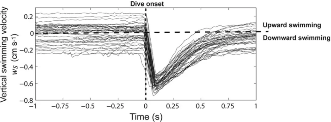
Using our quantitative definition of diving, we found that 82 larvae (of 874 total larvae) dove at least once during their observed trajectory in the unforced regime, and 57 larvae (of 1019 total larvae) dove at least once in the forced regime. We overlaid the diving trajectories aligned by dive onset time in the unforced regime (Fig. 2) to identify similarities in diving trajectories, and found similar timescales in the downward acceleration for all larvae, on the order of 0.1 s. Larvae reached peak downward velocities ranging from20.5 to 20.7 cm s21 and decelerated to zero velocity in approxi-mately 1 s. Prior to dive onset, larvae engaged in a range of vertical velocities, centered near zero, but both upward and downward swimming were observed, suggesting that larvae

had no fixed pre-dive behavior. As larvae decelerated from the dive and resumed a more constant vertical velocity, they exhibited a similar range of vertical velocities, indicating that larvae also had no fixed post-dive behavior. Vertical displacement from a single dive was of order 1021 _{cm, or} approximately four body lengths, and comparable to the Kolmogorov scale, the length scale of the smallest eddies in the forced regime.

Hydromechanical parameters triggering the dive response A range of temporal intervals prior to the dive onset was investigated, from 0.33 s to 3 s, in intervals of 0.33 s (see Sup-porting Information) to identify potential reaction time-scales for diving larvae. A hydromechanical parameter was considered to be a consistent trigger to the dive response only if (1) it differed significantly between diving and non-diving larvae in the specified temporal interval, and (2) this significant response held in both flow regimes, unforced and forced, for identical temporal intervals.

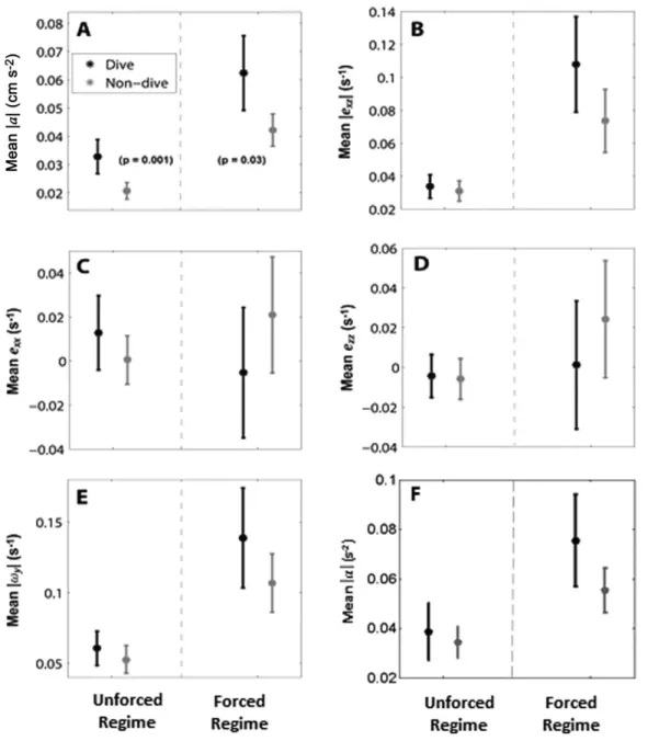
Diving larvae consistently experienced significantly higher mean fluid acceleration than non-diving larvae. In the unforced regime, mean accelerations were significantly higher for diving larvae in the 1 s, 1.33 s, 1.66 s, and 2 s time intervals and intermittently significant for longer time inter-vals (Table 1; Fig. 3A). In the forced regime, mean accelera-tions were significantly higher for diving larvae in all time intervals from 1.33 s to 3 s prior to the dive onset (Table 1; Fig. 3A). The intersection of these temporal intervals is 1.33– 2.33 s, representing the consistent response range in which diving larvae experienced significantly higher acceleration than non-diving larvae. For subsequent analyses presented in the main text, we used a central point of this interval, 1.66 s prior to dive onset, as the averaging window and denote the mean acceleration experienced by a larva in this interval as jaj_1:66.

No other hydromechanical parameter differed signifi-cantly prior to dive onset between diving and non-diving larvae (Fig. 3B–F, Supporting Information Tables A1, A2) in

Fig. 2.Diving larval vertical swimming velocity time series in the unforced regime, aligned by dive onset time. Larvae display strong uniformity in time spent accelerating downward, maximum downward velocity, and time spent decelerating out of the dive. Larvae exhibit a range of vertical swimming velocities prior to dive onset.

contrast to acceleration (Fig. 3A; Table 1). That is, none of shear deformation, normal deformation (horizontal or verti-cal), vorticity, or angular acceleration induced a diving response in larvae in any temporal window examined.

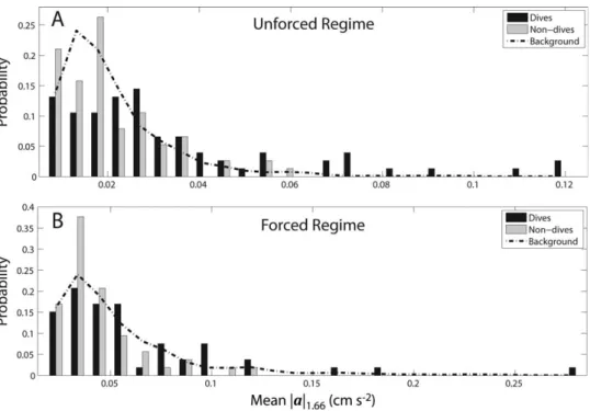
Flow accelerations experienced by diving and non-diving larvae in the 1.66 s interval were then compared to back-ground acceleration fields (Fig. 4). These three distributions of flow acceleration, Pðjaj1:66jlarva divesÞ, Pðjaj1:66jlarva does

not diveÞ, and Pðjaj1:66Þ, were significantly different in the

unforced regime (Table 2). A post hoc multiple comparison test of these distributions demonstrated that diving larvae experienced significantly higher average flow accelerations than both non-diving larvae and the average background acceleration. Non-diving larvae experienced flow accelera-tions that were indistinguishable from the background acceleration. In the forced regime, a similar pattern was observed: diving larvae experienced higher accelerations than did non-diving larvae, as well as higher accelerations than those occurring in the background flow. However, the result in this regime was non-significant (Table 2), likely

due to the smaller sample size of dives and lower power of the multiway comparison.

These distributions were then used to compute

Pðlarva dives j jaj_1:66Þ, the conditional probability that larvae dove for a given acceleration averaged over the 1.66 s pre-dive window in the unforced regime (Fig. 5). The posi-tive relationship between this probability and the accelera-tion demonstrates that diving became a more probable response as mean fluid acceleration experienced by larvae increased. The bounds on the 95% confidence intervals increased for high acceleration values due to the rarity of high acceleration events, which likely also accounted for overestimates of the conditional diving probability (i.e., greater than 1) for high accelerations. The computation is omitted for the forced regime as the large decrease in num-ber of dives observed renders estimates much more uncertain.

Discussion

Comparisons of flow fields experienced by diving and non-diving larvae strongly support a conclusion that flow acceleration triggers the dive response in oyster larvae. Div-ing larvae experienced significantly higher mean fluid accel-erations than did non-diving larvae during a short period leading up to the dive onset in both turbulence regimes. The other candidate hydromechanical parameters did not differ significantly between diving and non-diving larvae: none of mean normal strain rates, shear strain rate, vorticity, or angular acceleration triggered the dive response. An exami-nation of diving in the central 1.66 s response window dem-onstrated that not only did diving larvae experience higher accelerations than non-diving larvae, but that these accelera-tions were anomalously high compared to the background (significantly so in the unforced regime). The correspon-dence between probability of diving and increasing fluid acceleration further reinforces the interpretation that diving is triggered by acceleration. Further, the time interval over which the threshold mean acceleration was experienced was important for triggering the dive response. When accelera-tion was averaged over temporal windows shorter than 1.33 s, higher acceleration did not appear to induce diving preferentially. This analysis suggests that the reaction time-scale of the larvae to the fluid acceleration field they experi-ence was at least 1.33 s. A lack of pattern in timescales longer than 2 s suggests that the larvae are responding to an acceleration event, roughly 1.5 s before the dive, rather than to mean acceleration over a longer interval.

The observation that a mean acceleration of 0.035 cm s22 triggered a dive in the unforced case, but not in forced case, indicates that the required threshold acceleration changes with the turbulence level. In the low-forcing regime, an aver-age acceleration of 0.06 cm s21 triggered a dive, while non-diving larvae experienced mean accelerations of 0.04 cm s22.

Table 1.

acceleration distributions experienced by diving vs. non-diving larvae, where means are computed in the stated window prior to dive onset. The null hypothesis states that mediansMd5Mnd

while the alternate hypothesis states that they differ. Signifi-cance level isa50.05, with bold results indicating significant p-values. The medians of mean acceleration distributions are sig-nificantly higher for diving larvae than non-diving larvae in both flow regimes, given at least a 1.33 s window over which local acceleration is averaged. Time interval prior to dive onset (s) Turbulence regime Rank sum z p-value 0.33 Unforced regime e!0 cm2s23 6314 1.84 0.06 0.66 6270 1.67 0.09 1.00 6490 2.48 0.01 1.33 6735 3.39 <0.001 1.66 6697 3.25 0.001 2.00 6406 2.17 0.02 2.33 6148 1.22 0.21 2.66 6626 2.99 0.002 3.00 6318 1.88 0.06 0.33 Forced regime e51023 cm2s23 3095 1.63 0.10 0.66 3076 1.51 0.13 1.00 3015 1.13 0.25 1.33 3166 2.08 0.03 1.66 3164 2.07 0.03 2.00 3325 3.08 0.002 2.33 3232 2.50 0.01 2.66 3144 1.94 0.05 3.00 3244 2.57 0.009

This result suggests that larvae become conditioned to the flow regime in which they find themselves, and the dive response is triggered by anomalously high accelerations com-pared to the background acceleration. This interpretation is supported by the finding that the accelerations experienced by diving larvae were significantly higher than both

non-diving larvae and the background field. In a previous study (Wheeler et al. 2013), the dive response was found to disap-pear entirely in highly turbulent flow conditions (having energy dissipation rates greater than 1021 cm2 s23). While our experimental results do not provide a complete explana-tion for this disappearance, we offer several possibilities.

Fig. 3.Values of hydromechanical parameters (mean and 95% confidence intervals) for diving larvae (black) and non-diving larvae (grey) in unforced and forced regimes. Values are calculated in a 1.66 s time interval prior to the dive onset in diving larvae, and a randomly selected 1.66 s time interval in the trajectories of non-diving larvae. Sample sizes aren582 for both groups in the unforced regime, andn557 in the forced regime. (A) Mean acceleration magnitudejajis significantly different between diving and non diving larvae for both turbulence regimes (seeTable 1). (B) Mean shear strain rate magnitudejexzjexperienced by diving and non-diving larvae is not significantly different in either turbulence regime (Supporting Informa-tion Table A2). (C–D) Mean horizontal and vertical normal strain ratesexxandezzexperienced by diving and non-diving larvae are not significantly dif-ferent in either turbulence regime (Supporting Information Table A1). (E) Mean vorticity magnitudejxyjexperienced by diving and non-diving larvae is not significantly different in either turbulence regime (Supporting Information Table A2). (F) Mean angular acceleration magnitudejajexperienced by diving and non-diving larvae is not significantly different in either turbulence regime (Supporting Information Table A2).

First, larvae may simply stop reacting to an acceleration trig-ger above a certain threshold which occurs in the higher tur-bulence regimes. Second, recall that larvae respond to anomalously high accelerations within a turbulence level, and this threshold increases with turbulence intensity, at least in unforced and low forcing conditions. The frequency

with which larvae encounter sufficiently high acceleration anomalies in more turbulent regimes may be lower, which would explain the lack of diving in these regimes. However, we cannot quantify the diving threshold accelerations for these higher flow regimes (beyond supposing the thresholds are greater than that observed in our low flow forced regime), and as such, this explanation for the lack of diving in high turbulence remains speculative. Alternatively, it is

Fig. 4.Probability distributions of mean flow acceleration magnitude experienced by larvae in a 1.66 s time interval (prior to dives for diving larvae, randomly selected for non-diving larvae), in unforced (A) and forced (B) regimes, respectively. The black bar distributions are those of diving larvae,

Pðjaj1:66jlarva divesÞ, the grey bar distributions are those of non-diving larvae,Pðjaj1:66jlarva does not diveÞ, and the black dashed curves are back-ground mean acceleration magnitudesPðjaj1:66Þ. Note the different acceleration scales in unforced and forced regimes.

Table 2.

acceler-ations experienced by the following three groups: diving larvae in a 1.66 s window prior to dive onset, non-diving larvae in a ran-dom 1.66 s window, and four fixed spatial points over all three experiments in a random 1.66 s window. The null hypothesis states that medians of all three mean acceleration distributions are equal, and the alternate hypothesis states that the mean accel-erations experienced by these groups are different. Significance level isa50.05, with bold results indicating significant p-values.

Source SS df MS v2 p Unforced regime Group 5:543104 2 2:773104 12.40 0.002 Error 9:713105 228 4:263104 Total 1:023106 ₂₃₀ Forced regime Group 9:763103 2 4:883103 4.38 0.11 Error 3:513105 _{160 2:19310}3 Total 3:603105 162

Fig. 5.Probability of larval dive conditioned on jaj1:66, the local mean acceleration field (averaged over 1.66 s window), i.e.,

Pðlarva divesj jaj1:66Þ, for the unforced regime. Larvae were more likely to dive when they encountered higher local flow acceleration. Shaded grey region represents the 95% confidence interval for all mean accelerations.

possible that the experimental setup precluded detection of dives because larvae are advected quickly in more highly tur-bulent flow. It is possible that it becomes more difficult to observe the diving response because larvae remain in the FOV for shorter time periods (although more larvae are observed in higher turbulence regimes).

The dive response for all observed larvae was highly uni-form in terms of acceleration and deceleration timescales (Fig. 2), and the response is predictable based on fluid accel-eration through the probability Pðlarva dives j jajÞ. These characteristics make the dive response well suited for inclu-sion into individual based models of larval behavior in com-plex flow fields (see for instance Koehl et al. 2007). Such models would be very useful for testing whether diving affects settlement success in simulated turbulent flow fields over rough bottom topography. The strong uniformity of the dive further suggests that the response, once instigated, is regulated by biomechanical constraints, as all larvae emerge from the dive and resume swimming on comparable timescales. In this way, the diving response triggered by acceleration may differ from the sinking response to water-borne chemical cues observed in the larval sea slug Phestilla sibogae(Hadfield and Koehl 2004). These larvae retract velar lobes instantly in response to coral-conditioned seawater, and continue to sink unless the cue is absent on timescales of 1 s or longer. Our larvae, conversely, cease to dive after approximately 1 s regardless of local flow conditions. While the larvae are capable of diving multiple times in succession, their behavior appears distinct from the sustained sinking observed inP. sibogaelarvae.

The effects of local environmental conditions on the behavior of mollusc larvae have been previously studied in a few species with varying results. Two bivalve larvae ( Crassos-trea gigas and Mytilus edulis) exposed to horizontal suction flow demonstrated no discernible swimming response as they approached a suction tube (Troost et al. 2008), a flow that would have a strong acceleration signal. However, the flow fields experienced by these larvae were quantified in a separate experiment from the larval observations. This tech-nique can make it difficult to isolate larval behavior (Wheeler et al. 2013), as small scale temporal and spatial var-iations in the flow field that larvae might experience are not captured. P. sibogae retract their velar lobes in response to mechanical stimulus (Hadfield and Koehl 2004), and poten-tially to local hydrodynamic conditions (M. Koehl pers. comm.), as well as the potentially distinct response to chem-ical cues, as discussed above. The similarity of the response (retraction of ciliated swimming organ into a shell) in differ-ent mollusc groups suggests that larval diving in response to acceleration may be common to multiple species.

A dive response when larvae are experiencing anomalously high accelerations could potentially be a beneficial strategy if they need to settle onto rough bottom surfaces, or to avoid predator feeding currents. We consider both possibilities,

beginning with the ecological implications of diving as a set-tlement response. PIV measurements over rough topography in an oscillating flow tank have demonstrated that the high-est accelerations occur up to 5 cm from the bottom, and decay rapidly farther above (R. Pepper, J. Jaffe, E. Variano, and M. Koehl pers. comm.). Further, simulated larvae in the PIV-measured flow experience peak accelerations of short duration that are much higher in magnitude than the mean values, much like the anomalously high accelerations experi-enced by the diving larvae in our study. The threshold accel-erations experienced by larvae in our unforced and forced regimes are small compared to the fluid accelerations near the bottom reported by Pepper et al., but may help larvae navigate downward through the water column at heights above 5 cm from the bottom. The dive response disappears in more highly turbulent flow regimes that more closely mimic the energetics of flow immediately above preferred settle-ment sites (e.g., Whitman and Reidenbach 2012), which offers further evidence the dive response is likely to be employed by larvae higher in the water column.

Larvae could alternatively experience flow acceleration due to suction feeding flows from predators in the plankton (Kiørboe et al. 1999; Jakobsen 2001; Holzman and Wain-wright 2009) or even from the feeding currents of adult oys-ters on reefs (Troost et al. 2008). In this way, the dive could act as an escape response analogous to the jumping behavior of copepods (e.g., Waggett and Buskey 2007; Lee et al. 2010) or the rapid downward swimming of insect larvae and pupae (e.g., Awasthi et al. 2012) observed in the presence of preda-tors. Larval dive responses to flow acceleration in the water column could thus increase larval supply to the seafloor, by either increasing the rate of downward flux, or decreasing the proportion lost to predators.

References

Awasthi, A. K., C.-H. Wu, and J.-S. Hwang. 2012. Diving as an anti-predator behavior in mosquito pupae. Zool. Stud. 51: 1225–1234.

Butman, C. 1987. Larval settlement of soft-sediment inverte-brates: The spatial scales of pattern explained by active habitat selection and the emerging role of hydrodynami-cal processes. Oceanogr. Mar. Biol.25: 113–165.

Butman, C., J. Grassle, and C. Webb. 1988. Substrate choices made by marine larvae settling in still water and in a flume flow. Nature333: 771–773. doi:10.1038/333771a0 Chan, K. 2012. Biomechanics of larval morphology affect

swimming: Insights from the sand dollars Dendraster excentricus. Integr. Comp. Biol.52: 458–469. doi:10.1093/ icb/ics092

Chia, F., R. Koss, and L. Bickell. 1981. Fine structural study of the statocysts in the veliger larva of the nudibranch,

Rostanga pulchra. Cell Tissue Res.214: 67–80. doi:10.1007/ BF00235145

Finelli, C., and D. Wethey. 2003. Behavior of oyster ( Crassos-trea virginica) larvae in flume boundary layer flows. Mar. Biol.143: 703–711. doi:10.1007/s00227-003-1110-z Fuchs, H. L., E. J. Hunter, E. L. Schmitt, and R. A. Guazzo.

2013. Active downward propulsion by oyster larvae in tur-bulence. J. Exp. Biol. 216: 1458–1469. doi:10.1242/ jeb.079855

Galtsoff, P. S. 1964. The American OysterCrassostrea virginica

(Gmelin). U.S. Fish Wildl. Serv. Fish. Bull.64: 1–480. Gross, T., and A. Nowell. 1985. Spectral scaling in a tidal

boundary layer. J. Phys. Oceanogr. 15: 496–508. doi: 10.1175/1520-0485(1985)015<0496:SSIATB>2.0.CO;2 Hadfield, M., and M. Koehl. 2004. Rapid behavioral

responses of an invertebrate larva to dissolved settlement cue. Biol. Bull.207: 28–43. doi:10.2307/1543626

Holzman, R., and P. Wainwright. 2009. How to surprise a copepod: Strike kinematics reduce hydrodynamic disturb-ance and increase stealth of suction-feeding fish. Limnol. Oceanogr.54: 2201–2212.doi:10.4319/lo.2009.54.6.2201 Jakobsen, H. 2001. Escape response of planktonic protists to

fluid mechanical signals. Mar. Ecol. Prog. Ser.214: 67–78. doi:10.3354/meps214067

Jonsson, P., C. Andre, and M. Lindegarth. 1991. Swimming behavior of marine bivalve larvae in a flume boundary-layer flow: Evidence for near-bottom confinement. Mar. Ecol. Prog. Ser.79: 67–76. doi:10.3354/meps079067 Kennedy, V. S. 1996. Biology of larvae and spat, p. 371–421.

InV. S. Kennedy, R. I. E. Newell and A. F. Eble [eds.], The Eastern Oyster (Crassostrea Virginica). Maryland Sea Grant. Kiørboe, T., and A. Visser. 1999. Predator and prey

percep-tion in copepods due to hydromechanical signals. Mar. Ecol. Prog. Ser.179: 81–95. doi:10.3354/meps179081 Kiørboe, T., E. Saiz, and A. Visser. 1999. Hydrodynamic

sig-nal perception in the copepod Acartia tonsa. Mar. Ecol. Prog. Ser.179: 97–111. doi:10.3354/meps179097

Koehl, M. 2007. Mini review: Hydrodynamics of larval settle-ment into fouling communities. Biofouling 23: 357–368. doi:10.1080/08927010701492250

Koehl, M., J. Strother, M. Reidenbach, J. Koseff, and M. Hadfield. 2007. Individual-based model of larval transport to coral reefs in turbulent, wave-driven flow: Behavioral responses to dissolved settlement inducer. Mar. Ecol. Prog. Ser.335: 1–18. doi:10.3354/meps335001

Lee, C.-H., H.-U. Dahms, S.-H. Cheng, S. Souissi, F. G. Schmitt, R. Kumar, and J.-S. Hwang. 2010. Predation of

Psudodiaptomus annandalei (Copepoda: Calanoida) by the grouper fish fryEpinephelus coioidesunder different hydro-dynamic conditions. J. Exp. Mar. Biol. Ecol. 393: 17–22. doi:10.1016/j.jembe.2010.06.005

Metaxas, A., and M. Saunders. 2009. Quantifying the bio-components in biophysical models of larval transport in

marine benthic invertebrates: Advances and pitfalls. Biol. Bull.216: 257–272.

Maxey, M. R., and J. J. Riley. 1983. Equation of motion for a small rigid sphere in a non-uniform flow. Phys. Fluids26: 883–889. doi:10.1063/1.864230

Nowell, A., and P. Jumars. 1984. Flow environments of aquatic benthos. Annu. Rev. Ecol. Syst. 15: 303–328. doi: 10.1146/annurev.es.15.110184.001511

Pedley, T., and J. Kessler. 1992. Hydrodynamic phenomena in suspensions of swimming microorganisms. Annu. Rev. Fluid Mech. 24: 313–358. doi:10.1146/annurev.fluid. 24.1.313

Thompson, R., R. I. E. Newell, V. S. Kennedy, and R. Mann. 1996. Reproductive processes and early development, p. 335–370. In V. S. Kennedy, R. I. E. Newell and A. F. Eble [eds.], The Eastern Oyster (Crassostrea Virginica). Maryland Sea Grant.

Troost, K., R. Veldhuizen, E. Stamhuis, and W. Wolff. 2008. Can bivalve veligers escape feeding currents of adult bivalves? J. Exp. Mar. Biol. Ecol. 358: 185–196. doi: 10.1016/j.jembe.2008.02.009

Waggett, R. J., and E. J. Buskey. 2007. Calanoid copepod escape behavior in response to a visual predator. Mar. Biol.150: 599–607. doi:10.1007/s00227-006-0384-3 Wheeler, J. D., and others. 2013. Upward swimming of

com-petent oyster larvae (Crassostrea virginica) persists in highly turbulent flow as detected by PIV flow subtraction. Mar. Ecol. Prog. Ser. 488: 171-185. doi:10.3354/ meps10382

Whitman, E. R., and M. A. Reidenbach. 2012. Benthic flow environments affect recruitment of Crassostrea virginica

larvae to an intertidal oyster reef. Mar. Ecol. Prog. Ser. 463: 177–191. doi:10.3354/meps09882

Acknowledgements

Thanks to Elaine Luo, Brenna McGann, Susan Mills, Andre Price, and Anthony Ritchie for assistance with larval acquisition, culture, experi-ments, and thanks to Anna Wargula for turbulence tank measurements. Thanks to Margaret Byron, Karen Chan, Joseph Fitzgerald, Mimi Koehl, and Evan Variano for helpful discussions throughout this project, and two anonymous reviewers for suggestions. We gratefully acknowledge the culturing expertise of the Aquaculture Research Corporation in Den-nis, Massachusetts, who supplied the larval oysters used in this study. This work was supported by NSF grant OCE-0850419, NOAA Sea Grant NA14OAR4170074, grants from the WHOI Coastal Ocean Institute, dis-cretionary WHOI funds, a WHOI Ocean Life Fellowship to LM, and a Grove City College Swezey Fellowship to EA.

Submitted 9 September 2014 Revised 23 February 2015 Accepted 6 April 2015 Associate editor: Josef D. Ackerman