Multipurpose small area estimation

(1)

M

ULTIPURPOSE

S

MALL

A

REA

E

STIMATION

H

UKUM

C

HANDRA

,

R

AY

C

HAMBERS

A

BSTRACT

Sample surveys are generally multivariate, in the sense that they measure more than one response variable. In theory, each variable can then be assigned an optimal weight for estimation purposes. However, it is often a distinct practical advantage to have a single weight that is used with all variables collected in the survey. This paper describes how such multipurpose sample weights can be constructed when small area estimates of the survey variables are required. The approach is based on the model-based direct (MBD) method of small area estimation described in Chambers and Chandra (2006). Empirical results reported in this paper show that MBD estimators for small areas based on

multipurpose weights perform well across a range of variables that are often of interest in business surveys. Furthermore, these results show that the proposed approach is robust to model misspecification and also efficient for the variables ill-suited to standard methods of small area estimation (e.g. variables that contain a significant proportion of zeros).

(2)

Multipurpose Small Area Estimation

Hukum Chandra1 and Ray Chambers2

1. Southampton Statistical Sciences Research Institute University of Southampton

Highfield, Southampton, SO17 1BJ, UK

2. Centre for Statistical and Survey Methodology University of Wollongong

Wollongong, NSW, 2522, Australia

August 15 2006

Abstract

Sample surveys are generally multivariate, in the sense that they collect data on more than one response variable. In theory, each variable can then be assigned an optimal weight for estimation purposes. However, it is a distinct practical advantage to have a single weight for all variables collected in the survey. This paper describes how such multipurpose sample weights can be constructed when small area estimates of the survey variables are required. The approach is based on the model-based direct (MBD) method of small area estimation described in Chambers and Chandra (2006). Empirical results reported in this paper show that MBD estimators for small areas based on multipurpose weights perform well across a range of variables that are often of interest in business surveys. Furthermore, these results show that the proposed approach is robust to model misspecification and also efficient when used with variables that are not suited to standard methods of small area estimation (e.g. variables that contain a significant proportion of zeros).

Keywords: Multivariate surveys, Multipurpose sample weights, MBD approach, Mixed

(3)

1. Introduction

The weights that define the best linear unbiased predictor (BLUP) for the population total of a variable of interest (see Royall, 1976) depend on the population level conditional variance/covariance matrix for that variable. Unless this matrix is always proportional to a known matrix, this optimality is variable specific. However, most surveys are multivariate, and it is often an advantage to have a common weight for all response variables. This is especially true where linear estimates are produced using the survey data. In what follows we refer to such weights as ‘multipurpose’.

When a sufficiently rich set of auxiliary variables exist, and response variables can be assumed to be conditionally uncorrelated given these variables, multipurpose weights can be constructed by fitting a linear model for each response variable in terms of the complete set of auxiliary variables. See Chambers (1996). An essentially equivalent idea is to use a calibrated set of sample weights, where the calibration is with respect to these auxiliary variables. See Deville and Särndal (1992).

(4)

2. Optimal Multipurpose Sample Weighting

2.1 Basic Concepts and Notation

Consider a population U consisting of N units, each of which has a value of a characteristic of interest y associated with it. The population vector yU =(y1,...,yN)! is

treated as the realisation of a random vectorYU =(Y1,...,YN)!, and our aim is estimation

of the total T_y = _j! y_j

U

"

(or meanY =N!1

y_j

j"U

#

) of the values definingy_U. A sample

s of n units is selected from U, and the y values of the sample units are observed. We denote the set of N – n non-sampled population units by r. We assume the availability ofXU, an N×p matrix of values of p auxiliary variables that are related, in some sense,

to the values inyU. In particular, yUand XU are related by the general linear model E(yU)= XU! and Var(yU)=VU (1)

where ! is a p!1 vector of unknown parameters and VU is a positive definite

covariance matrix. Without loss of generality, we arrange the vector yU so that the first n elements correspond to the sample units, writingyU! =(y!s y!r). We similarly partition

XU and VU according to sample and non-sample units as

XU = X_s X_r ! "

# $_%& and VU =

V_ss V_sr V_rs V_rr !

"

# $_%&.

Here Xs is the n! p matrix of sample values of the auxiliary variable, Vssis the n!n

covariance matrix associated with the n sample units that make up the n!1 sample vectorys. Corresponding non-sample quantities are denoted by a subscript of r, while

Vrs denotes the

(

N!n

)

"n matrix defined byCov(yr,ys). It is known (see Royall, 1976)

that among linear prediction unbiased estimators Tˆy= !wsys of Ty the variance of the

prediction error, Var( ˆT_y!T_y), is minimised by weights of the form

ws =1n +H!

(

XU!1N " !Xs1n

)

+

(

In" !HXs!

)

Vss "1_V

sr1N"n. (2)

Here H =

(

X_s!V_ss"1X_s

)

"1X!_sV_ss"1, 1_mis a vectors of ones of order m and I_n is the identity

matrix of order n. We refer to the weights (2) as the best linear unbiased prediction (BLUP) weights for y. By definition, these weights are calibrated on the variables in XU

(5)

model can be used to specify the covariance matrix components Vss and Vsr in (2), the

MBD approach to small area estimation (see Chambers and Chandra, 2006) uses these weights, with Vss and Vsr replaced by suitable estimates, to define direct estimates of

small area quantities.

2.2 Optimal Multipurpose Weighting for Uncorrelated Variables

Suppose we have K response variables and a common set of auxiliary variables with values defined by the population matrixXU, and that model (1) holds for each of them

(although with different parameter values). Suppose further that these variables are mutually uncorrelated. We use an extra subscript k k( =1,....,K) to denote quantities associated with the kth response variable, for example Vkss and wks denote respectively

the n!n covariance matrix and n!1 vector of sample weights that are associated with the n!1 vector yks of sample values of the k

th

response variable. With this notation, our aim is to derive an optimal set of multipurpose weights ws = {wj;j!s} for the K

response variables measured in the survey. Let T_k =1!_Ny_k denote the population total of

yk, with estimator Tˆk = !wsyks based on these multipurpose weights. The weights ws are

then said to be !-optimal if (a) E( ˆTk!Tk)=0 for each value of k, and (b) the !

-weighted total prediction variance

#

_k!_kVar( ˆTk "Tk) is minimised at ws. Here !k is a

user-specified non-negative scalar quantity that reflects the relative importance attached

to the kth_{response variable, with} !_k k

"

=1.

Put a_s =w_s !1_s. In order to derive an explicit expression for the !-optimal multipurpose weights we first note that under (a)

E( ˆT_k!T_k)=E(a"_sy_ks! "1_N_!_ny_kr)=E(a_s"X_s ! "1_N_!_nX_r)#_k =0$ a"_sX_s =1"_N_!_nX_r. (3)

Furthermore, the prediction variance for estimator Tˆk = !wsyks is then

Var( ˆTk!Tk)=E(as"yks! "1N!nykr)

2 =

Var(a"syks! "1N!nykr)+[E(a"syks! "1N!nykr)]

2

. The second term on the right hand side above vanishes under (3), so that

Var( ˆTk!Tk)=a"sVar(yks)as !2as"Cov(yks,ykr)1N!n+1"N!nVar(ykr)1N!n

(6)

We use the method of Lagrange multipliers to minimise (4) subject to (3). The corresponding Lagrangian loss function is

!(1) = "k _#

asVkssas$2a#sVksr1N$n

{

}

k=1 K

%

+2(as#Xs $ #1N$nXr)& (5)

where ! is a vector of Lagrange multipliers. Differentiating (5) with respect to a_s and setting the result equal to zero leads to

!"(1)

!as

$

! a_s = !_kV_kss

k=1 K

"

(

)

#1

!kVksr k=1 K

"

1_N_#_n-X_s$

{

}

(6)

Multiplying both sides of (6) on the left by Xs! and using (3), we see that

!

Xsas = Xs! _k₌₁"kVkss K

#

(

)

$1

"kVksr k=1

K

#

1N$n

(

)

$ !Xs _k₌₁"kVkss K

#

(

)

$1

Xs%

! Xr!1N"n = X!sU1

"1

W11N"n" !XsU1

"1

Xs#

! != Xs"U1

!1_W

11N!n-U1

!1_X_s"₌ _U 1

!1_W 1-U1

!1_X

s Xs#U1 !1_X

s

(

)

!1

#

XsU1 !1_W

1! #Xr

{

}

$

% &'1N!n

=U1

!1

Xs Xs"U1

!1

Xs

(

)

!1

"

X1N ! "Xs1n

(

)

+ In-U1

!1

Xs Xs"U1

!1

Xs

(

)

!1

"

Xs

#

$ %&U1

!1

W11N!n.

That is, the optimal multipurpose sample weights are given by

ws

(1) ₌

1n+H1!

(

XU!1N " !Xs1n

)

+

[

In-H1!Xs!

]

U1 "1

W11N"n (8)

where H1= X!sU1 "1_X

s

(

)

"1

! XsU1

"1₌ _X_!

s _k=₁#kVkss K

$

(

)

"1

Xs

{

}

"1

!

Xs _k=₁#kVkss K

$

(

)

"1

.

Observe that the analytical form of the optimal multipurpose weights (8) is similar to the variable specific BLUP weights (2), except that Vkssand Vksr are replaced by the

weighted sums U1 =

"

_k!kVkss and W1 =

"

_k!kVksr respectively. Clearly (8) reduces to

(7)

2.3 Optimal Multipurpose Weighting for Correlated Variables

Survey variables are correlated in general. Let Ckl =Cov(yk,yl). The obvious

generalization of the !-weighted total prediction variance to this case leads to the loss function

!1, !2,.... !K

(

)

" # !

(

1, !2,.... !K

)

(9)

where elements of the matrix !={!_kl} are given by

!kl =

Var( ˆTk-Tk) if k=l

Cov( ˆTk-Tk, ˆTl-Tl) if k"l

# $ % &%

and we now have

Cov( ˆT_k!T_k, ˆT_l!T_l)=a"_sC_klssa_s !2a"_sC_klsr1_N_!_n+1"_N_!_nC_klrr1_N_!_n. The Lagrange function to be minimized in this case is

!(2) ₌ _"

1, "2,.... "K

(

)

# $ "

(

1, "2,.... "K

)

+2(a#sXs% #1N%nXr)& = !kVar( ˆTyk "Tyk)

k

#

+ !k !lCov( ˆTyk "Tyk, ˆTyl "Tyl)

l$k

#

k

#

)as *

"

k !kVksr

+ !k !lCklsr

l#k

"

k

"

$ % & ' (

)1N*n +Xs+=0

! U₂a_s !W₂1_N_!_n+X_s"=0

! a_s =U₂!1

(

W₂1_N_!_n-X_s"

)

(11)

.

Proceeding as in the uncorrelated case then leads to the optimal multipurpose weights for correlated survey variables

ws

(2) ₌

1n +H2!

(

XU!1N " !Xs1n

)

+

[

In-H!2Xs!

]

U2 "1

W21N"n (12)

where H2 = Xs!U2

"1

Xs

(

)

"1

!

XsU2

"1

. As in the uncorrelated variables case, we note that the

(8)

that in this case V_kss and V_ksr are replaced by U2 = !kVkss k

"

+ !k !lCklss

l#k

"

k

"

and

_j_!_s wkj

i

"

(13)

where s_i denotes the sample (of size n_i) in area i and the weights w_kj are calculated

using (2), substituting estimated values Vˆkss and Vˆksr for the corresponding components

of the covariance matrix of the population values of this variable. In order to define these estimates, we assume that these population values follow the linear mixed model

YkU = XU!k+ZUuk +ekU (14)

where YkU =(Yk!,1,...,Yk!,m)!, XU =(X1!,....,Xm!)!, ZU =diag(Zi;1!i!m),

uk =(uk,1,...,uk,m)! and ekU =(ek,1,...,ek,m)! denote partitioning into area ‘components’.

Here uk,i is a random effect associated with area i, with Var(uk,i)= !u,kIN_i, and ek,i is

the vector of individual random effects for area i, with Var(e_k,i)= !_e,kI_N

i . It follows that

Var(Yk,i)=Vk,i =!e,kIN_i +Zi!u,kZi". The variance components !e,k and !u,k can be

estimated from the sample data using standard methods (maximum likelihood, restricted maximum likelihood, i.e. REML, or method of moments). Substituting these estimated variance components back into the definition of Vk,i and noting that

V_k =diag(V_k_,_i;1!i!m) then leads to a corresponding estimate of this population level

(9)

In order to use the multipurpose weights (8) and (12) in MBD estimation, we assume that the survey variables all follow the linear mixed model (14), with normal random effects. Furthermore, for any two variables of interest, say the kth

and lth

, area and individual random effects remain uncorrelated but now

uki uli

! "#

$

%& !MVN(0,'u) with !u =

Var(uki)

Cov(uli,uki)

" #$

Cov(uki,uli)

Var(uli)

% &' = !u,kk !u,kl " #$ !u,kl !u,ll % &' (15) and e_kij elij ! "# $

%& !MVN(0,'e) with !e=

Var(e_kij) Cov(elij,ekij)

" #$

Cov(e_kij,e_lij) Var(elij)

% &' =

!e,kk

!e,kl

" #$

!e,kl

!e,ll

%

&'. (16)

Hence

Vk,i =Var(Yk,i)=!e,kkIN_i +Zi!u,kkZi"

Vl,i =Var(Yl,i)=!e,llIN_i +Zi!u,llZi"

and

Ckl,i =Cov(Yk,i,Yl,i)=!e,klIN_i +Zi!u,klZi".

(10)

formulae above then enables us to compute U1, W1, U2 and W2, and hence the

multipurpose weights (8) and (12). Computation of MBD estimates for the small area means of the different survey variables is then straightforward using (13), with these multipurpose weights replacing the variable specific EBLUP weights there.

As noted earlier, the multipurpose weights (8) and (12) are essentially EBLUP type weights based on ‘importance averaging’ of the variance and covariance components associated with the different survey variables. This motivates us to consider a second approach to deriving multipurpose weights based on corresponding ‘importance averaging’ of the variable specific EBLUP sample weights (2) for these variables. That is, we simply define our multipurpose weights as the importance-weighted average of the variable specific weights (2) across all K survey variables. This leads to weights

w_s(3) ₌ !

kwsk

k

"

(17)

where wsk denotes the value of (2) for the k

th

survey variable and !_k denotes the

relative importance of this variable, with !k

k

"

=1.

3. An Empirical Study

In this section we report on a design-based simulation study that illustrates the performance of small area MBD estimation combined with multipurpose weights. The basis of this study is the same target population of N = 81982 farms, the same 1000 independent replications of a stratified random sampling design with overall sample size n=1652 and the same m = 29 small areas of interest (defined by agricultural regions) that underpin the simulation results reported in Chandra and Chambers (2005). Note that regional sample sizes in this design are fixed from simulation to simulation but vary between regions, ranging from a low of 6 to a high of 117, and hence allowing an evaluation of the performance of the different methods considered across a range of realistic small area sample sizes. See Chandra and Chambers (2005) for more details.

(11)

cattle on the farm, (vi) Sheep = number of sheep on the farm, (vii) Equity = total farm equity (A$), and (viii) Debt = total farm debt (A$). Our aim is to estimate the average of these variables in each of the 29 different regions. In doing so, we use the fact that these regions can be grouped into three zones (Pastoral, Mixed Farming, and Coastal), with farm area (hectares) known for each farm in the population. This auxiliary variable is referred to as Size in what follows.

Although the linear relationship between the eight target variables and Size is rather weak in the population, this improves when separate linear models are fitted within six post strata. These post-strata are defined by splitting each zone into small farms (farm area less than zone median) and large farms (farm area greater than or equal to zone median). The mixed model (14) was therefore specified so that the matrix XU of

auxiliary variable values included an effect for Size, effects for the post-strata and effects for interactions between Size and the post strata. Two different specifications for

ZU (corresponding to whether a random slope on Size was included or not) were

considered. We refer to these as model I and as model II respectively below. We use REML estimates of random effects parameters, obtained via the lme function in R (Bates and Pinheiro, 1998) when fitting (14) to individual survey variables. When fitting the multivariate mixed models defined by (15) and (16) we use the method of moments (Rao, 2003).

(12)

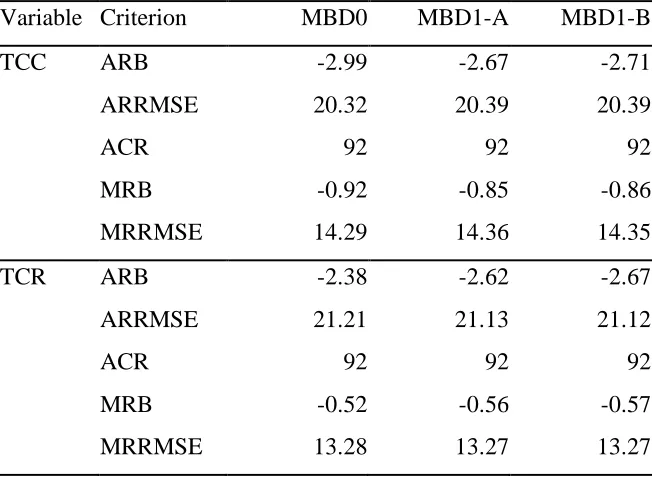
The simulation study was carried out in five stages. In the first stage, model I was assumed and the performance of the three estimators MBD0, MBD1-A and MBD1-B for two variables (TCC and TCR) was investigated to see if there were gains to be had from exploiting correlations among the survey variables. As noted earlier, we used the method of moments (Henderson’s Method 3) to estimate model parameters in this case. Results from this stage are set out in Table 1. In the second stage of the study we compared the performance of the four estimation methods EBLUP, MBD0, MBD1-A and MBD2 under models I and II for the 5 response variables (TCC, TCR, FCI, Cattle and Sheep) where both models can be fitted. Results from this stage are presented in Tables 2 and 3 and in Figure 1. Note that the remaining three target variables in the study (Crops, Equity and Debt) are not suited to linear modeling via (14) under model II because of the presence of large numbers of zeros. Consequently, in the third stage of the study, we used the multipurpose weights derived in the second phase (i.e. weights based on the K

= 5 variables TCC, TCR, FCI, Cattle and Sheep) in MBD1-A to evaluate the performance of this estimator for the three variables Crops, Equity and Debt that were impossible to model using model II. Results from this stage are shown in Table 4 and in Figure 2. In the fourth stage we used the fact that model I can be fitted to all eight variables to define multipurpose weights that we then use in MBD1-A. Results from this stage are presented in Table 5 and in Figure 2. Note that in all four of these simulation stages, we assign equal importance to all variables included in derivation of the multipurpose weights. Consequently, in the final simulation (stage five) we replicated the stage two simulation for MBD1-A, but this time assigned weights to each variable proportional to its population variability.

Table 1 about here

(13)

with different levels of correlation support this conclusion. Consequently the simulation results presented below focus on MBD1-A.

Tables 2 and 3 about here

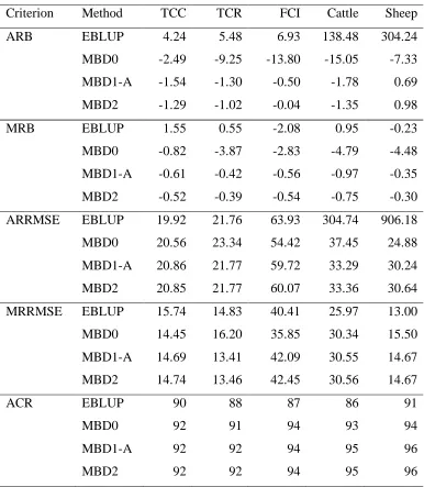
In the second stage of the simulation study, we compared the two variable specific methods EBLUP and MBD0 with the two multipurpose methods MBD1-A and MBD2. Tables 2 and 3 show the summary performances generated by these four methods for the five variables TCC, TCR, FCI, Cattle and Sheep under Models I and II respectively. Under the better fitting Model II (Table 3), multipurpose method MBD1-A performs marginally better than multipurpose method MBD2, which in turn is slightly better than the variable specific MBD0. All three are often substantially better than EBLUP for these data. Under Model I (Table 2), the two multipurpose methods MBD1-A and MBD2 record substantially better bias performances than the variable specific MBD0 and EBLUP, and better to comparable performances with respect to mean squared error. Overall, the multipurpose method MBD1-A seems the weighting method of choice for these five variables and these data.

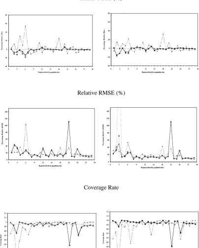
In Figure 1 we show the regional level performances of EBLUP, MBD0, MBD1-A and MBD2 when estimating average TCC under model I and model II. Note the relatively better performance of all methods under model II. A considerable reduction in relative biases under multipurpose weighting can also be seen in most regions. A similar pattern of results was observed for TCR, FCI, Cattle and Sheep.

Figure 1 about here

(14)

The unstable performance of EBLUP for the Cattle and Sheep variables in Tables 2 and 3 is also noteworthy. Upon investigation we found that these anomalous results were due to the presence of large numbers of negative estimates in some of the regions, which in turn were caused by zero values in the data.

Table 4 about here

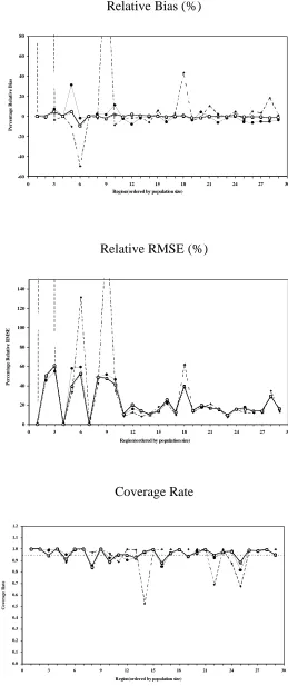
As noted earlier, our results suggest that multipurpose estimation based on MBD1-A is preferable to that based on MBD2. Consequently, in Table 4 we contrast the performances of the variable specific estimators EBLUP and MBD0 with that of the multipurpose estimator MBD1-A for the three variables (Crops, Equity and Debt) that contain a large number of zeros, and so were not included in calculation of the multipurpose weights used in MBD1-A. Note that these results are based on model I, since model II cannot be used for these variables. We see that MBD1-A is again clearly the method of choice, with EBLUP performing particularly badly - as one might expect given the large number of zero values in the data for Crops, Equity and Debt. This is evident when we look at Figure 2, which shows the regional specific performances of the three methods for Crops. Here we see that the EBLUP method fails in regions 2, 6, 9 and 18. These are regions where there are a large number of zero values for this variable.

Figure 2 about here

In the results presented so far, the multipurpose weights used in the MBD1-A method have been based on the K = 5 target variables that were ‘suited’ to linear mixed modeling with the model II specification. However, if a model I specification is used, we can use all K = 8 target variables to define these weights via (8). In Table 5 therefore we compare the performance of the MBD1-A method under this model with weights obtained by using both the limited (K = 5) and full (K = 8) set of target variables in (8). This shows that these weights are quite insensitive to this choice. The almost imperceptible regional differences between the Crops estimates defined by these two sets of weights (see Figure 2) reinforces this observation. Similar region-specific performances were observed for Equity and Debt as well.

(15)

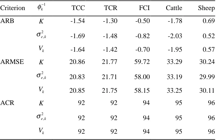
So far, when computing the multipurpose weights, we have assigned equal importance to all K target variables that are used to define them. However, a reasonable alternative approach would be to assign importance factors based on the intrinsic variability of these variables. Two natural options in this regard are !_k =1 /"e,k

2

and !_k =1 / Vk, where !e,k

2

and Vk are the individual and total variability of the k

th

target variable. Table 6

provides summary details of the performance of the MBD1-A method when the multipurpose weights (based on TCC, TCR, FCI, Cattle and Sheep) are computed using these alternative importance weighting factors. These results show that, for the population considered in the simulation study, there is little to choose between these different importance weighting factors.

Table 6 about here

4. Summary and Further Research

(16)

Acknowledgements

The first author gratefully acknowledges the financial support provided by a PhD scholarship from the U.K. Commonwealth Scholarship Commission.

References

Bates, D.M. and Pinheiro, J.C. (1998). Computational methods for multilevel models. Available from http://franz.stat.wisc.edu/pub/NLME/

Chambers, R.L. (1996). Robust case-weighting for multipurpose establishment surveys.

Journal of Official Statistics12, 3 - 32.

Chambers, R. and Chandra, H. (2006). Improved direct estimators for small areas. Submitted for publication.

Chandra, H. and Chambers, R. (2005). Comparing EBLUP and C-EBLUP for small area estimation. Statistics in Transition, 7, 637-648.

Deville, J. C. and Särndal, C.-E. (1992). Calibration estimators in survey sampling.

Journal of the American Statistical Association87, 376 - 382.

Prasad, N.G.N and Rao, J.N.K. (1990). The estimation of the mean squared error of small-area estimators. Journal of the American Statistical Association, 85, 163-171. Rao, J. N. K. (2003). Small Area Estimation. New York: Wiley.

Royall, R.M. (1976). The linear least-squares prediction approach to two-stage sampling. Journal of the American Statistical Association, 71, 657-664.

(17)

[image:17.595.141.467.196.435.2]

Table 1 Average relative bias (ARB), median relative bias (MRB), average relative root mean squared error (ARRMSE), median relative root mean squared error (MRRMSE) and average coverage rate (ACR) generated by MBD0, MBD1-A and MBD1-B for TCC and TCR under model I. All averages and medians are expressed as percentages and are over the 29 regions of interest.

Variable Criterion MBD0 MBD1-A MBD1-B TCC ARB -2.99 -2.67 -2.71 ARRMSE 20.32 20.39 20.39

ACR 92 92 92

MRB -0.92 -0.85 -0.86 MRRMSE 14.29 14.36 14.35 TCR ARB -2.38 -2.62 -2.67 ARRMSE 21.21 21.13 21.12

ACR 92 92 92

(18)

[image:18.595.111.497.192.635.2]

Table 2 Average relative bias (ARB), median relative bias (MRB), average relative root mean squared error (ARRMSE), median relative root mean squared error (MRRMSE) and average coverage rate (ACR) for the five variables best suited to linear mixed modelling. All averages and medians are expressed as percentages and are over the 29 regions of interest. Model I is assumed.

(19)

[image:19.595.110.497.193.635.2]

Table 3 Average relative bias (ARB), median relative bias (MRB), average relative root mean squared error (ARRMSE), median relative root mean squared error (MRRMSE) and average coverage rate (ACR) for the five variables best suited to linear mixed modelling. All averages and medians are expressed as percentages and are over the 29 regions of interest. Model II is assumed.

(20)

[image:20.595.160.447.197.542.2]

Table 4 Average relative bias (ARB), median relative bias (MRB), average relative root mean squared error (ARRMSE), median relative root mean squared error (MRRMSE) and average coverage rate (ACR) for EBLUP, MBD0 and MBD1-A for Crops, Equity and Debt under model I. All averages are expressed as percentages and are over the 29 regions of interest.

Criterion Methods Crops Equity Debt ARB EBLUP 90.31 4.36 8.39 MBD0 0.00 -9.32 -4.94 MBD1-A -0.21 -1.20 -0.96 MRB EBLUP 0.00 -0.28 1.16 MBD0 -0.84 -3.51 -2.36 MBD1-A 0.00 -0.32 -0.61 ARRMSE EBLUP 123.96 18.51 29.02 MBD0 23.53 19.14 27.71 MBD1-A 22.92 17.05 28.57 MRRMSE EBLUP 15.10 12.32 21.49 MBD0 15.76 16.18 23.70 MBD1-A 15.80 13.52 24.88 ACR EBLUP 95 88 91

MBD0 96 92 93

(21)

Table 5 Average relative bias (ARB), average relative root mean squared error (ARRMSE) and average coverage rate (ACR) for multi-purpose weighting (MBD1-A) based on original K = 5 and extended K = 8 variable sets under model I.

Variable K = 5 K = 8

[image:21.595.101.507.154.366.2]

(22)

Table 6 Average relative bias (ARB), average relative root mean squared error (ARRMSE) and average coverage rate (ACR) for multi-purpose weighting (MBD1-A) under !_k =1 / K, !_k =1 /"e,k

2

and !_k =1 / V_k for K = 5 target variables (TCC, TCR, FCI,

Cattle, Sheep) under model I.

Criterion !k"1 TCC TCR FCI Cattle Sheep ARB K -1.54 -1.30 -0.50 -1.78 0.69

!e,k 2

-1.69 -1.48 -0.82 -2.03 0.52

Vk -1.64 -1.42 -0.70 -1.95 0.57

ARMSE K 20.86 21.77 59.72 33.29 30.24

!e,k 2

20.83 21.71 58.00 33.19 29.99

Vk 20.85 21.75 58.15 33.25 30.11

ACR K 92 92 94 95 96

!e,k

2

92 92 94 95 96

[image:22.595.116.493.180.424.2]

(23)

Figure 1 Regional performance of EBLUP (dashed line), MBD0 (thin line), MBD1-A (thick line) and MBD2 (dotted line) for TCC under model I (left) and model II (right).

Relative Bias (%)

-40 -20 0 20 40 60 80

0 3 6 9 12 15 18 21 24 27 30 Region(ordered by population size)

P e r c e n ta g e R e la ti v e B ia s -40 -20 0 20 40 60 80

0 3 6 9 12 15 18 21 24 27 30

Region(ordered by population size)

P e r c e n ta g e R e la ti v e B ia s

Relative RMSE (%)

0 20 40 60 80 100 120 140

0 3 6 9 12 15 18 21 24 27 30

P e r c e n ta g e R e la ti v e R M S E 0 20 40 60 80 100 120 140

0 3 6 9 12 15 18 21 24 27 30

P e r c e n ta g e R e la ti v e R M S E Coverage Rate 0 0.1 0.2 0.3 0.4 0.5 0.6 0.7 0.8 0.9 1 1.1 1.2

0 3 6 9 12 15 18 21 24 27 30

C o v e r a g e R a te 0.0 0.1 0.2 0.3 0.4 0.5 0.6 0.7 0.8 0.9 1.0 1.1 1.2

0 3 6 9 12 15 18 21 24 27 30

[image:23.595.98.502.145.649.2]

(24)

[image:24.595.165.424.136.753.2]

Figure 2 Regional performances of EBLUP (dashed line), MBD0 (thin line), MBD1-A under K = 5 (thick line) and MBD1-A under K = 8 (dotted line) for Crops under model I.

Relative Bias (%)

-60 -40 -20 0 20 40 60 80

P er ce n ta g e R el a ti v e B ia s

Relative RMSE (%)

0 20 40 60 80 100 120 140

P er ce n ta g e R el a ti v e R M S E Coverage Rate 0.0 0.1 0.2 0.3 0.4 0.5 0.6 0.7 0.8 0.9 1.0 1.1 1.2