Ansgar Belke is Associate Senior Research Fellow at CEPS and Full Professor of Macroeconomics and Director of the Institute of Business and Economic Studies (IBES) at the University of Duisburg-Essen. Since 2012 he is (ad personam) Jean Monnet Professor. Jens Klose is Professor for Statistics and Economics at the THM Business School, Giessen, Germany.
This paper was originally published in the Journal of Common Market Studies, May 2017. CEPS is republishing it here with the kind permission of the JCMS.
CEPS Working Documents give an indication of work being conducted within CEPS’ research programmes and aim to stimulate reactions from other experts in the field. The opinions expressed in this document are the sole responsibility of the authors and do not necessarily represent the official position of CEPS.
978-94-6138-615-1
Available for free downloading from the CEPS website (www.ceps.eu) © CEPS 2017
Equilibrium Real Interest Rates
and Secular Stagnation:
An Empirical Analysis for Euro-Area Member Countries
Ansgar Belke and Jens Klose
No 2017/09, August 2017
Abstract
Is secular stagnation—a period of persistently lower growth such as that seen following the financial crisis of 2008-09—a valid concern for euro-area countries? We tackle this question using the well-established Laubach-Williams model to estimate the unobservable equilibrium real interest rate and compare it to the actual real rate. In light of the considerable increase in heterogeneity among EU member countries since the beginning of the financial crisis, we apply our approach to 12 euro-area countries to provide country-level answers to the question of secular stagnation. The presence of secular stagnation in a number of euro-area countries has important implications for ECB decision-making (e.g. voting power in the Governing Council) and EU governance. Our results indicate that secular stagnation is not a significant threat to most euro-area countries, with the possible exception of Greece.
Keywords: equilibrium real interest rate, secular stagnation, euro-area countries, heterogeneity
1. Introduction ... 1
2. Equilibrium real interest rates and secular stagnation ... 3
3. The data issue ... 8
4. Results ... 9
4.1 Output gap ... 9
4.2 Ex-ante real interest rates ... 10
4.3 Ex-post real interest rates ... 15
5. Conclusions ... 18
References ... 20
Annex 1. The Laubach-Williams Model ... 23
[image:2.595.70.524.131.339.2]List of Tables and Figures Table 1. Parameter estimates ... 4
Figure 1. Real interest rates and secular stagnation ... 6
Figure 2. One- and two-sided output gap estimates ... 10
Figure 3. Ex-ante real rates and one-sided equilibrium estimates ... 11
Figure 4. Ex-ante real rates and two-sided equilibrium estimates ... 14
Figure 5. Ex-post real rates and one-sided equilibrium estimates ... 16
1
Equilibrium Real Interest Rates and
Secular Stagnation:
An Empirical Analysis for Euro-Area
Member Countries
Ansgar Belke and Jens Klose
CEPS Working Document No 2017/09, June 2017
1. Introduction
Can a sustained period of low growth be expected in euro-area countries? As in other industrialized countries, growth rates declined substantially in the wake of the financial crisis and appear to have moved to a lower trajectory since that time. In euro-area countries, this decline has been quite heterogeneous. Some countries like Greece, Portugal, and Spain have been hit harder than others by the financial crisis and subsequent European debt crisis.
To account for this phenomenon of lower economic growth, economists have reinvented the secular stagnation hypothesis (Summers, 2014a). For a survey and deeper analysis of this issue, see Teulings and Baldwin (2014). The central tenet of this hypothesis is that there is a difference between the real interest rate, the decisive variable for investment and consumption decisions, and its equilibrium value. Summers (2014a) and others believe that the equilibrium real rate declined substantially in the crisis period and is now far into the negative range and thus too low for the actual real rate to be reached. In this situation, secular stagnation occurs and investments and savings can no longer be balanced.
Although the equilibrium real rate is an unobservable variable, there is a straightforward way to estimate it. Laubach and Williams (2003) introduced a model for estimating this rate in the US that we apply here to twelve euro-area countries. Moreover, we compare our results to ex-ante and ex-post real interest rates to determine whether some euro-area countries are being confronted with secular stagnation.
Heterogeneity among euro-area member countries also has implications for the euro area as a whole, in particular for common monetary policy.1 Especially during the peak of the crisis, there was a widespread feeling that the ECB's policy was not meeting the needs of any of its member countries.
If secular stagnation can only be identified in certain member countries while others are returning to solid growth, the ECB has to decide how to deal with this issue by applying the monetary policy that is best for the euro area as a whole. However, in such an environment, this may not be optimal for every member country. For example, if the ECB decides to help countries in secular stagnation by adopting an accommodative monetary policy, other countries may soon face inflation pressures. If, on the other hand, the ECB steers its monetary policy towards the non-secular-stagnation countries, thus employing a restrictive monetary policy, the countries experiencing secular stagnation might become even more depressed.
This heterogeneity among euro-area member countries has important bearings for the voting decisions of the Governing Council of the ECB since these become even more intransparent in conjunction with the rotation model introduced in 2015.2 The reason is simple: national central bank presidents are presumed to vote for monetary policies that correspond with their respective countries’ national preferences. In a situation of high heterogeneity among the countries, this means a wide array of different interests and thus strongly diverging views of what constitutes the best monetary policy. This is exacerbated with the rotation model since at one given meeting, a coalition could be found for a more loose monetary policy and at the next (where other governors are allowed to vote), there could be a coalition for a tighter monetary policy. This could lead to bias in the inflation expectations.
As far as the preferences of national central bank presidents (NBPs) are concerned, the literature generally considers a broader measure of macroeconomic divergence than merely the inflation rate preferences of member states (see, e.g., Bénassy-Quéré and Turkisch, 2009). Authors usually apply the Taylor rule to simulate NBPs’ desired interest rates, which in our case depend on the estimated equilibrium interest rates. This method is often interpreted as a good approximation of future preferences of NBPs and represents the future macroeconomic developments better than past inflation rates. Our estimation of EMU member-country-specific equilibrium interest rates is also important for authors such as Kosior, Rozkrut and Torój (2008), who use information on interest rate preferences in order to define coalitions in the Governing Council and calculate power indices such as the Shapley-Shubik index. In these exercises, the “neutral” levels of real interest rates are often simply set equal to the long-term rates of real GDP growth (see, for instance, Bénassy-Quéré and Turkisch, 2009, pp. 46–51). We feel that our method of calculating the equilibrium real interest rates of the EMU member countries represents clear progress over this practice.
1 See Drudi et al. (2012) on the crisis response of the ECB and its connections to fiscal reforms and financial stability.
See Heinemann and Hüfner (2004) and Gros and Hefeker (2002) more generally on national divergence of preferred interest rates and ECB interest rate policy.
2 See Belke and Styczynska (2006) on the issue of voting power allocation in the ECB Governing Council when the
But even on the fiscal side, increasing heterogeneity has important implications for the governance of the European Union. While there is evidence that EU economic policy has been conducted primarily on an intergovernmental level in the crisis, neglecting previously existing structures of economic governance (Dawson, 2015),3 it is even more difficult to implement such a policy when the economic situation and thus political preferences of the leaders diverge. The recent refugee crisis might be seen as a good example in this respect. In recent years, however, a number of economic reforms have been undertaken to strengthen the European Monetary Union (Lane, 2012). These include the Fiscal Compact, the Macroeconomic Imbalance Procedure, and the introduction of a banking union.
For all these reasons, which present challenges to European economic governance, it is important to look at the economic situation of the euro-area member countries at the national level. Whether secular stagnation is present in none of these countries, in only a few, or in (almost) all countries is therefore important to know from a policy perspective. This paper proceeds as follows: First, we explain the role of the real interest rate and its equilibrium value in the context of secular stagnation and discuss possible drivers of secular stagnation. Second, we explain the data we use in our empirical specification. And third, we present and discuss our results. The final section concludes.
2. Equilibrium real interest rates and secular stagnation
The financial crisis of 2008-09 depressed output in leading developed countries considerably. But even after the most severe tensions had been eased, output growth remained persistently lower than before the crisis. This phenomenon may be explained by a permanent drop in potential output, and has been referred to as “secular stagnation” (Summers, 2014a, 2014b, 2014c; Teulings and Baldwin, 2014).4
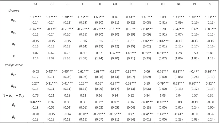
The secular stagnation hypothesis focuses on the real interest rate and its equilibrium value. Under normal circumstances, both should be equalized at the point where aggregate investments equal aggregate savings. However, in a crisis period, and even afterwards, this may no longer be the case. The reason for this is quite simple. While the equilibrium real rate floats freely, the actual real rate faces a lower bound. The latter is due on the one hand to the zero lower bound on nominal interest rates, because individuals can hold excess savings in cash rather than in their bank accounts, thus generating a nominal interest rate of zero. On the other hand, inflation rates or, more precisely, inflation expectations are too low to generate significantly negative real rates. For example, in the euro area, inflation expectations are mainly anchored at about 2 percent, being the inflation target of the ECB.5
3 Auel and Höing (2014) found that the treatment of parliamentarian scrutiny of EU-reforms if they were asked in the
recent crisis has not changed compared to pre-crisis scrutiny.
4 In fact, Summers was not the first to detect a secular stagnation. This term goes back to the 1930s, where Hansen
(1939) first developed this theory in what may be considered a similar situation.
5 This being said, one way to significantly lower the actual real rates is to increase the inflation target. For example
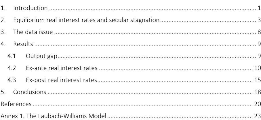
Table 1. Parameter estimates
AT BE DE FI FR GR IR IT LU NL PT SP
IS-curve
𝛼𝑦,1 1.22***
(0.14) 1.37*** (0.24) 1.70*** (0.11) 1.73*** (0.13) 1.68*** (0.10) 0.16 (0.11) 0.44** (0.22) 1.40*** (0.08) 0.89 (0.81) 1.47*** (0.09) 1.40*** (0.16) 1.83*** (0.15)
𝛼𝑦,2 -0.47***
(0.15) -0.42* (0.24) -0.75*** (0.10) -0.76*** (0.11) -0.72*** (0.10) 0.73*** (0.10) 0.38** (0.19) -0.58*** (0.09) 0.20 (0.92) -0.47*** (0.07) 0.32* (0.16) -0.83*** (0.12)
𝛼𝑟 -0.15
(0.15) -0.15 (0.13) -0.15 (0.18) -0.16 (0.14) -0.16 (0.15) -0.15 (0.12) -0.15 (0.15) -0.16*** (0.02) -0.06*** (0.01) -0.15 (0.11) -0.15 (0.17) -0.15 (0.16) 𝑐 1.07 (1.14) 0.62 (1.32) 0.76 (1.35) 0.50 (1.07) 0.82 (1.24) 1.37*** (0.20) 1.46*** (0.21) 0.69** (0.23) 0.51*** (0.07) 1.28 (1.06) 0.50 (1.02) 0.81 (1.12) Phillips-curve
𝛽𝜋,1 -0.03
(0.17) 0.48*** (0.11) 0.40*** (0.08) 0.62*** (0.07) 0.68*** (0.08) 0.32** (0.14) 0.35*** (0.07) 0.06 (0.09) 0.76*** (0.00) 0.38*** (0.08) -0.47* (0.24) 0.36*** (0.11)
𝛽𝜋,2 0.27*
(0.14) 0.31*** (0.11) 0.41*** (0.11) 0.25** (0.11) 0.16* (0.09) 0.34** (0.17) 0.53*** (0.13) 0.10 (0.06) -0.79*** (0.00) 0.58*** (0.13) 0.90*** (0.12) 0.32** (0.15)
1 − 𝛽𝜋,1− 𝛽𝜋,2 0.76 0.21 0.19 0.13 0.16 0.34 0.12 0.84 1.03 0.04 0.57 0.32
𝛽𝑦 0.46***
Variance
𝜎1 0.0731 0.2207 0.0612 0.1288 0.0534 0.0039 0.8433 0.1166 0.8987 0.0000 0.0044 0.0000
𝜎2 0.0699 0.1668 0.1190 0.1507 0.1400 0.2696 0.6036 0.2023 0.0028 0.1274 0.0000 0.2094
𝜎3 0.3997 0.1536 0.6665 0.9408 0.1085 1.1946 0.5164 0.3187 0.0038 1.2125 1.4487 0.3797
𝜎4 0.0011 0.0005 0.0012 0.0011 0.0002 0.0096 0.0016 0.0059 0.0000 0.0004 0.0016 0.0060
𝜎5 0.0000 0.0010 0.0003 0.1485 0.0006 0.0000 0.0004 0.0000 0.0000 0.0000 0.1154 0.0000
𝜆𝑔 0.0531 0.0594 0.0431 0.0335 0.0431 0.0894 0.0548 0.1357 0.0232 0.0184 0.0333 0.1262
𝜆𝑧 0.0001 0.0001 0.0001 0.0001 0.0001 0.0001 0.0001 0.0001 0.0060 0.0001 0.1244 0.0001
𝑙𝑜𝑔
− 𝑙𝑖𝑘𝑒𝑙𝑖ℎ𝑜𝑜𝑑 -191.08 -227.89 -291.43 -268.35 -184.87 -235.89 -441.13 -339.13 -629.29 -334.16 -635.17 -244.60
However, if the equilibrium real interest rate falls below the lower bound of the actual real rate, there is no longer an equilibrium of aggregate investments and savings (Figure 1). In the euro area, this lower bound should be at about -2 percent. In this case, excess savings occur, depressing output or, more precisely, depressing potential output permanently. In other words, even more negative real interest rates are needed to balance savings and investments (Teulings and Baldwin, 2014).
Figure 1. Real interest rates and secular stagnation
Notes: i=real interest rate, I=aggregate investments, S=aggregate savings, approximately -2 percent as intercept is chosen because the minimum should be given at a zero nominal rate minus the ECB inflation target of about two percent.
The secular stagnation hypothesis assumes that with the financial crisis, either aggregate investments have fallen or aggregate savings have risen to levels that imply an equilibrium interest rate too low for the real rate to reach. Several factors that determine this development have been identified.
Second, a high degree of regulation in product markets may cause investments to be permanently depressed. However, these regulations can also be changed by the governing political parties. This can have a large effect, especially in the euro area (Jimeno et al., 2014 and Barnes et al., 2013). The same holds with respect to labour market reforms, which tend to increase employment. Moreover, long-term unemployment leads to skill atrophy (Eurosclerosis, Blanchard and Summers, 1986), thereby permanently lowering the potential rate of employment6 and potential growth (hysteresis).
Third, rising income inequality permanently increases savings, as individuals with high incomes have a higher marginal rate of saving (Summers, 2014b). This in turn tends to lower the equilibrium real rate, all else being equal.
Fourth, we observe a fall in investment prices, leading by construction to a downward shift in the investment curve (Summers, 2014b or Glaeser, 2014). These lower investment prices are simply due to the altered structure of investment goods. In a nutshell, investments in such IT-technologies as social networks are not as expensive as investments in industrial machinery.
Fifth, demographics are a crucial determinant, influencing both aggregate savings and investments. On the one hand, savings change according to the life-cycle hypothesis, which proposes that savings are highest in economies with a relatively large proportion of the population being close to retirement. Moreover, savings may rise with increasing life expectancy and uncertainty about future pension payments, irrespectively of the life cycle (Jimeno et al., 2014). On the other hand, investments fall in aging economies because revenue expectations drop when the population is about to shrink (Gros, 2014). According to Krugman (2014), this problem is especially severe in euro-area countries.
Finally, a low degree of innovation, measured as increases in total factor productivity, is observed in several industrial economies. If this is the case, investments should also be low because new machinery does not generate a significant benefit in comparison to older equipment. Gordon (2014), however, believes that low total factor productivity is the new normal rather than a temporary exception, and assumes lower growth rates on this basis. However, forecasting total factor productivity is a difficult task. Mokyr (2014) and Glaeser (2014), for example, argue that some innovations still have the potential to boost total factor productivity, such as information technology, biotechnology, or new materials.
But whether one or several of the factors are indeed able to lower the equilibrium real interest rate to levels too low for the actual real rate to reach is mainly an empirical question. For this purpose, we employ the model most widely used in estimating the equilibrium real rate: the Laubach-Williams model.
6 In relation to the current context, see Draghi (2014), who explicitly mentions hysteresis in unemployment when
3. The data issue
The equilibrium real interest rate is an unobservable variable. Thus, it has to be estimated. Laubach and Williams (2003) established an estimation method for this variable that employs a state-space approach.7 It still is the most important model used in equilibrium real interest rate determination. Besides the unobservable equilibrium real interest rate, the unobservable potential output is also estimated in this procedure. The method is frequently used to estimate the equilibrium real interest rate.8 Also for the euro area, Mesonnier and Renne (2007), Garnier and Wilhelmsen (2009), Belke and Klose (2013), Beyer and Wieland (2015) and Holston et al. (2016) have used the model to find a measure of the equilibrium real interest rate. But to the best of our knowledge, up to now no one has employed this model to the various euro-area countries to account for possible heterogeneity in the monetary union. In the following, we try to fill this gap.
We estimate the model with respect to twelve euro-area countries, the eleven founding members of the euro area9 and Greece, which was the first country to join the monetary union in 2001. For the remaining seven current euro-area member countries, we were unable to find time series for all variables that dated long enough into the past to give us reliable estimates. For some of our twelve countries in the sample we obtained quarterly data dating back to 1970. However, this applies only to Finland, France, Germany, Italy, Luxembourg, Netherlands, and Portugal, while the sample period begins for Belgium in 1975Q3, for Ireland in 1976, for Spain in 1977, for Austria in 1980, and for Greece in 1989. All sample periods proved to be long enough to generate reliable results. The end of the sample period is 2015Q4 for all countries under investigation, owing to issues of data availability.
For each of these countries, we have collected the data on real GDP, consumer prices, energy prices and interest rates. All data is seasonally adjusted and taken from the OECD database. As the relevant interest rate we use the three-month interbank rate in line with studies in this field. Since the countries in question have not had their own interbank rates since the euro area was established, we added the data of the three month EURIBOR for all dates where each respective country was a member of the monetary union, that is, from 1999 for the eleven founding members and from 2001 for Greece.
Our interpretation of the results is based on a comparison of the estimated equilibrium real rate and the observed real rate. For this purpose, we make use of two concepts in measuring the latter: ex-ante and ex-post real rates. The former represents the nominal interest rate minus the expected inflation, which in our case are adaptive expectations and thus lagged inflation rates (𝑟𝑡 = 𝑖𝑡− 𝜋𝑡−1), while the latter is formulated as the interest rate minus the observed inflation rate until maturity (𝑟𝑡 = 𝑖𝑡− 𝜋𝑡).10 Even though the real interest rates
7 See the annex for the Laubach-Williams model and its implementation in the current context.
8 See, e.g., Trehan and Wu (2004), Clark and Kozicki (2005), Kiley (2015) or Laubach and Williams (2015) for the US.
Holston et al. (2016) estimate the model for the US, Canada, the UK, and the euro area.
differ depending on the concept used, this will have only a minor influence on the results, i.e., whether or not secular stagnation may be a relevant problem in a euro-area member country.
4. Results
In this section, we present the estimation results of our model for the equilibrium real interest rate and compare these to the observed real interest rates.
As in Laubach and Williams (2003), we will present the results for the unobserved variables using a one-sided (predicted) measure and a two-sided (smoothed) version. One-sided estimates make use only of the data prior to the respective point in time, while the two-sided version uses data from the whole sample period. Although the estimated time series differ depending on which method is used, the policy implications remain the same for both indicators. We proceed by showing the results separately for the unobserved state variables, starting with the potential output/output gap, before turning to the ex-ante and ex-post equilibrium real interest rates.
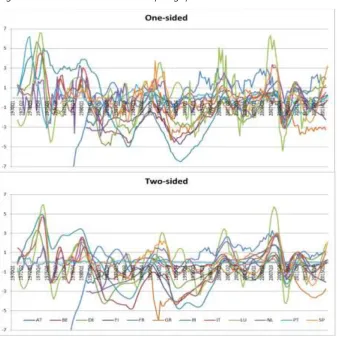
4.1 Output gap
Our estimates of the output gaps, starting for most countries in the 1970s, are given in Figure 2. Rather than commenting in detail on the results for the whole sample period,11 we restrict our analysis to the recent financial crisis period beginning in 2008-09. Note, moreover, that the results do not depend on whether a one-sided or two-sided approach is chosen, but that our estimation results are fairly robust across specifications.
As becomes obvious, several countries produced above potential before 2008, so the output gap was positive. These included Spain and Ireland, which would later become crisis countries, but also Luxembourg and the Netherlands.
However, with the financial crisis reaching its apex in 2009, all output gaps turn negative. Moreover, all countries exhibit a rebound in their output gap in 2010. But during the European debt crisis, we see a more heterogeneous evolution of the output gap in the countries under investigation. While the Greek output gap in particular remains negative until the end of the sample, this holds to a lesser extent for other crisis countries. What is more, in some other crisis countries there seems to be a turnaround in 2012-13, so output gaps start rising again, and some now even turn positive, as in the case of Ireland and Spain. Besides Greece, at the end of the sample period only Finland shows a substantially negative output gap, while the output gap seems to be closed for most of the other countries. On the other hand, Spain, Ireland, Luxembourg, and Germany tend to reveal the highest positive output gaps by the end of 2015. Thus our output gaps are in the end a bit more positive than those of the European Commission.
11 But please note that our estimates are generally in line with those of international organisations using a production
Figure 2. One- and two-sided output gap estimates
Notes: One-sided=predicted estimates, two-sided=smoothed estimates; AT=Austria, BE=Belgium, DE=Germany, FI=Finland, FR=France, GR=Greece, IR=Ireland, IT=Italy, LU=Luxembourg, NL=Netherlands, PT=Portugal, SP=Spain.
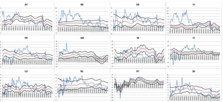
4.2 Ex-ante real interest rates
Figure 3. Ex-ante real rates and one-sided equilibrium estimates
Second, in the wake of the financial crisis of 2008-09, real interest rates became negative for all countries, at least in some quarters. The lowest real interest rate was about -2 percent, which may be considered the empirical lower bound as indicated in Section 2.12 However, negative real rates are far from being rare in the history of the euro-area countries. In the 1970s in particular, we frequently observe negative real interest rates in all countries where we have data for this longer sample period.
This overall trend of low rates in the 1970s, higher rates in the 1980s and early 1990s, and declining rates thereafter is also mirrored by our estimates of the equilibrium real rates. With these findings, we are in line with those of Laubach and Williams (2003) for the US and Mesonnier and Renne (2007) for the euro area, to cite two examples. This being said, it is clear that the real rates and their equilibrium values do not differ substantially. Apart from some countries in some periods (e.g., Belgium, Finland, and Luxembourg in the 1980s or Italy in the 1970s), the observed real rates are mainly found to lie within the one standard deviation band of the equilibrium real interest rate.1314 This holds especially since the financial crisis period began. We observe in most countries that the real rates and the equilibrium values fell further in this period, although the reduction in the former was even more pronounced. This does not come as a surprise, since the real rates are by definition more volatile than their equilibrium (or structural) counterparts. At the end of the sample, the equilibrium real interest rate is estimated to be slightly above zero for most countries. So there is, in our view, no indication that interest rates cannot fall as low as the equilibrium value, as the secular stagnation hypothesis would suggest. In addition, for most countries, real rates seem to be lower than the equilibrium values, reinforcing our conclusion that a phenomenon such as secular stagnation is absent for most euro-area countries.
If anything, there is one exception: that of Greece. For this country, we indeed observe a real rate that is substantially higher than the equilibrium value. Moreover, the value of the equilibrium rate is estimated to be around the level of -10 percent. Real rates can clearly not reach these low levels in Greece in the current context of a European monetary policy under zero interest rates and a price environment characterized by deflation rather than inflation due to falling personal incomes. So we have to conclude that Greece may indeed face some kind of secular stagnation, even though we also estimate that the equilibrium rate has been rising since 2013 and the upper bound of the standard deviation band is now almost equal to the real interest rate.
12 Note again that this empirical lower bound is consistent with a zero nominal interest rate and an inflation rate of
about 2 percent, as in the case of the ECB’s inflation target.
13 The standard deviation of the equilibrium real rate is computed in line with Laubach and Williams (2003) as σr∗=
√c²σ42+ σ52. Since those are only quarterly standard deviations, we added four of them up to yearly standard deviations in the figures.
14 Note, however, that this band is quite large for several countries, implying a large dispersion. But the finding is in
When we estimate the model and smooth the results using a two-sided filter, the results do not change significantly (Figure 4). The only difference is that estimates of the equilibrium real rate are less volatile, which is exactly what we expect when smoothing the time series.
Figure 4. Ex-ante real rates and two-sided equilibrium estimates
4.3 Ex-post real interest rates
Figure 5. Ex-post real rates and one-sided equilibrium estimates
Figure 6. Ex-post real rates and two-sided equilibrium estimates
5. Conclusions
In this contribution, we have tried to answer the question of whether euro-area countries have been facing symptoms of secular stagnation since the beginning of the financial crisis in 2008-09—a period of persistently lower growth. Based on our analysis of the difference between the real interest rate and its equilibrium value, we arrive at a surprisingly clear answer: most euro-area member countries do not face such a phenomenon. This is the case even though the equilibrium real rates have been falling since the mid-1990s, turning even as low as about minus two percent in the wake of the crisis. This is because the actual real rate, in principle, can do the same, and has de facto reached these low levels. So there is no reason to fear that “excess savings” may occur, because aggregate investments and savings cannot be equalized through the real interest rate.
This holds at least when comparing only the point estimates of the equilibrium real interest rate to the actual real rate. However, the estimation of the equilibrium real rate is subject to a considerable degree of uncertainty, as shown by our confidence bands in figures 3 to 6. For several countries, these reach negative levels. Thus, if the lower bound is taken into consideration, several countries may face secular stagnation.
But for one country, we can draw inferences even when comparing the point estimate with the actual real rate. For Greece, we indeed find equilibrium real rates of about -10 percent, which are clearly too low to be reached through the actual real interest rate. But these rates recovered afterwards, so at the end of the sample, the upper bound of our equilibrium rate uncertainty band is almost equal to the actual real rate. Greece may therefore face secular stagnation. What can be done about this? A European-wide policy such as a monetary stimulus is clearly not appropriate in addressing a specific problem that only one member country faces. The same holds with respect to fiscal reforms aimed at increasing the fiscal resources of EU institutions or the introduction of a European fiscal transfer system (Baskaran and Hessami, 2013). These kinds of reforms only increase the likelihood of bailout once a country encounters pressures that may in turn result in even higher borrowing. However, Greece has already received substantial financial support from other euro-area member countries, the International Monetary Fund, and European lending facilities (EFSF and ESM). Without this support, Greece would already be insolvent.
Greece should therefore undertake national reforms on their own in order to improve its economic situation. It may be that European institutions with the power to intervene in national budget plans if it judges them to be unsustainable will have to force the necessary reforms (Schuhknecht et al, 2011, Baskaran and Hessami, 2013). The Institutions of the International Monetary Fund, the European Commission, and the ECB are already performing such tasks today.
References
Auel, K. and Höing, O. (2014): Parliaments in the Euro Crisis: Can the Losers of Integration still Fight Back?, Journal of Common Market Studies, Vol. 52(6), pp.1184-1193.
Barnes, S., Bouis, R., Briard, P., Dougherty, S. and Eris, M. (2013): The GDP Impact of Reforms - A Simple Simulation Framework, OECD Economics Department Working Papers, No. 834.
Baskaran, T. and Hessami, Z. (2013): Monetary Integration, Soft Budget Constraints, and the EMU Sovereign Debt Crisis, University of Konstanz – Department of Economics Working Paper Series No. 2013-03.
Belke, A. and Klose, J. (2013): Modifying Taylor-Reaction Functions in the Presence of the Zero-Lower-Bound - Evidence for the ECB and the Fed, Economic Modelling, Vol. 35, pp. 515-527.
Belke, A. and Styczynska, B. (2006): The Allocation of Power in the Enlarged ECB Governing Council: An Assessment of the ECB Rotation Model, Journal of Common Market Studies, Vol. 44(5), pp. 865-897.
Bénassy-Quéré, A. and Turkisch, E. (2009): The ECB Governing Council in an Enlarged Euro Area, Journal of Common Market Studies, 47(1), pp. 25–53.
Beyer, R.C.M. and Wieland, V. (2015): Schätzung des mittelfristigen Gleichgewichtszinses in den Vereinigten Staaten, Deutschland und dem Euro-Raum mit der Laubach-Williams-Methode, SVR-Working Paper No. 03/2015.
Blanchard, O., Dell'Ariccia G. and Mauro, P. (2010): Rethinking Macroeconomic Policy, IMF Staff Position Note 10/03.
Blanchard, O. and Summers, L. (1986): Hysteresis and the European Unemployment Problem, in NBER Macroeconomics Annual, Vol. 1, pp. 15-78.
Clark, T.E. and Kozicki, S. (2005): Estimating Equilibrium Real Interest Rates in Real Time,
North American Journal of Economics and Finance, Vol. 16(3), pp. 395-413.
Dawson, M. (2015): The Legal and Political Accountability Structure of ‘Post-Crisis’ EU Economic Governance, Journal of Common Market Studies, Vol. 53(5), pp. 976-993.
Draghi, M. (2014): Unemployment in the Euro Area, Speech at the Annual Central Bank Symposium in Jackson Hole, 22. August 2014.
Drudi, F., Durré, A. and Mongelli, F.P. (2012): The Interplay of Economic Reforms and Monetary Policy: The Case of the Eurozone, Journal of Common Market Studies, Vol. 50(6), pp. 881-898.
Glaeser, E. (2014): Secular Joblessness, in "Secular Stagnation: Facts, Causes and Cures", VoxEU, pp. 69-82.
Gordon, R. (2014): The Turtle's Progress: Secular Stagnation Meets the Headwinds, in "Secular Stagnation: Facts, Causes and Cures", VoxEU, pp. 47-60.
Gros, D. (2014): Investment as the Key to Recovery in the Euro Area, CEPS Policy Briefs, 18. November 2014, Brussels.
Gros, D. and Hefeker, C. (2002): One Size Must Fit All: National Divergences in a Monetary Union, German Economic Review, Vol. 3(3), pp. 247-262.
Hamilton, J.D., Harris, E.S., Hatzius, J. and West, K.D. (2015): The Equilibrium Real Funds Rate: Past, Present and Future, NBER Working Paper, No. 21476, NBER, Cambridge, MA.
Hansen, A. (1939): Economic Progress and Declining Population Growth, American Economic Review, Vol. 29(1), pp. 1-15.
Heinemann, F. and Hüfner, F. P. (2004). Is the View from the Eurotower Purely European? National Divergence and ECB Interest Rate Policy, Scottish Journal of Political Economy, 51(4), pp. 544–558.
Hodrick, R. and Prescott, E. (1997): Post-War Business Cycles: An Empirical Investigation, Journal of Money, Credit and Banking, Vol. 29, pp. 1-16.
Holston, K., Laubach, T. and Williams J.C. (2016): Measuring the Natural Rate of Interest: International Trends and Determinants, FRBSF Working Paper, 2016-11.
Jimeno, J., Smets, F. and Yiangou, J. (2014): Secular Stagnation: A view from the Eurozone, in "Secular Stagnation: Facts, Causes and Cures", VoxEU, pp. 153-164.
Katsimi, M. and Moutos, T. (2010): EMU and the Greek Crisis: The Political-Economiy- Perspective, European Journal of Political Economy, Vol. 26(4), pp. 568-576.
Kiley, M.T. (2015): What Can the Data Tell Us About the Equilibrium Real Interest Rate?, Finance and Economics Discussion Series 2015-077, Board of Governors of the Federal Reserve System.
Koo, R. (2014): Balance Sheet Recession is the Reason for Secular Stagnation, in "Secular Stagnation: Facts, Causes and Cures", VoxEU, pp. 131-142.
Kosior, A., Rozkrut, M. and Torój, A. (2008). Rotation Scheme of the ECB Governing Council: Monetary Policy Effectiveness and Voting Power Analysis, in: Raport na temat pelnego uczestnictwa Rzeczpospolitej Polskiej w trzecim etapie Unii Gospodarczej i Walutowej, National Bank of Poland, August, pp. 53–102.
Lane, P.R. (2012): The European Sovereign Debt Crisis, Journal of Economic Perspectives, Vol. 26(3), pp. 49-68.
Laubach, T. and Williams J.C. (2003): Measuring the Natural Rate of Interest, Review of Economics and Statistics, Vol. 85(4), pp. 1063-1070.
Laubach, T. and Williams J.C. (2015): Measuring the Natural Rate of Interest Redux, FRBSF Working Paper, 2015-16.
Mesonnier, J.S. and Renne, J.P. (2007): A Time-Varying "Natural" Rate of Interest for the Euro Area, European Economic Review, Vol. 51, pp. 1768-1784.
Mokyr, J. (2014): Secular Stagnation? Not in your life, in "Secular Stagnation: Facts, Causes and Cures", VoxEU, pp. 83-90.
Schuhknecht, L., Moutot, P., Rother, P. and Stark, J. (2011): The Stability and Growth Pact: Crisis and Reform, ECB Occasional Paper No. 129.
Stock, J. (1994): Unit Roots, Structural Breaks and Trends, in Engle, R. and McFadden, D.,
Handbook of Econometrics, Vol. 4, pp. 2739-2841, Amsterdam.
Stock, J. and Watson, M. (1998): Median Unbiased Estimator of Coefficient Variance in a Time-Varying Parameter Model, Journal of the American Statistical Association, Vol. 93, pp. 349-358.
Summers, L. (2014a): U.S. Economic Prospects: Secular Stagnation, Hysteresis, and the Zero Lower Bound, Business Economics, Vol 49(2), pp. 65-73.
Summers, L. (2014b): Reflections on the "New Secular Stagnation Hypothesis", in "Secular Stagnation: Facts, Causes and Cures", VoxEU, pp. 27-38.
Summers, L. (2014c): Low Equilibrium Real Rates, Financial Crisis and Secular Stagnation, in "Across the Great Divide: New Perspectives on the Financial Crisis", pp. 37-50.
Trehan, B. and Wu, T. (2004): Time Varying Equilibrium Real Rates and Monetary Policy Analysis, FRBSF Working Paper, 2004-10.
Annex 1. The Laubach-Williams Model
The Laubach-Williams model we use consists of two signal equations and three state equations. All variables are measured as quarterly growth rates. The signal equation (1) is an IS-curve measuring the effect of the first two lags of the real interest rate gap (𝑟 − 𝑟∗) on the output gap (𝑌 − 𝑌̅). Additionally, two lags of the output gap are added to the equation. Equation (2) is the second signal equation, which measures a Phillips curve estimating the influence of the output gap on prices (𝜋). Moreover, the prices are assumed to vary with lagged energy prices (𝜋𝑜) since those are a crucial input factor in the production process.15 Again, lagged values of the dependent variable are added. In this case, and in line with Laubach and Williams (2003), we add eight lags assuming the second to fourth and fifth to eighth lags to have the same influence. Moreover, the coefficients of the lagged inflation rates are restricted to unity, in line with the aforementioned seminal paper.
𝑌𝑡− 𝑌̅𝑡= 𝛼𝑦,1(𝑌𝑡−1− 𝑌̅𝑡−1) + 𝛼𝑦,2(𝑌𝑡−2− 𝑌̅𝑡−2) +𝛼2𝑟[(𝑟𝑡−1− 𝑟𝑡−1∗ ) + (𝑟𝑡−2− 𝑟𝑡−2∗ )] + 𝜀1,𝑡 (1)
𝜋𝑡 = 𝛽𝜋,1𝜋𝑡−1+𝛽𝜋,2
3 (𝜋𝑡−2+ 𝜋𝑡−3+ 𝜋𝑡−4) +
1−𝛽𝜋,1−𝛽𝜋,2
4 (𝜋𝑡−5+ 𝜋𝑡−6+ 𝜋𝑡−7+ 𝜋𝑡−8) +
𝛽𝑦(𝑌𝑡−1− 𝑌̅𝑡−1) + 𝛽𝑜(𝜋𝑡−1𝑜 − 𝜋
𝑡−1) + 𝜀2,𝑡 (2)
𝑌̅𝑡 = 𝑌̅𝑡−1+ 𝑔𝑡−1+ 𝜀3,𝑡 (3)
𝑔𝑡 = 𝑔𝑡−1+ 𝜀4,𝑡 (4)
𝑧𝑡= 𝑧𝑡−1+ 𝜀5,𝑡 (5)
𝑟𝑡 = 𝑖𝑡− 𝜋𝑡−1 (6)
𝑟𝑡∗ = 𝑐𝑔
𝑡+ 𝑧𝑡 (7)
The state equations model the time-series generating process of the two unobservable variables, potential output and equilibrium real interest rate. The potential output 𝑌̅ is a
15 Laubach and Williams (2003) also use import prices as a variable in the Phillips curve. We are unable to proceed in
function of its lagged own value and its unobservable growth rate 𝑔 (Equation (3)). The growth rate of the potential output is in itself a state variable following a random walk (Equation (4)) as well as the last state variable 𝑧 (Equation (5)), measuring additional determinants of the equilibrium real rate, such as the time preference of households. The last two equations, (6) and (7), show how the real rate and its equilibrium value are built. In order to save degrees of freedom, the inflation expectations in the real rate are modelled simply by the using adaptive expectations, thus being the lagged inflation rate. This is in line with other studies estimating the equilibrium real rate for the euro area (Mesonnier and Renne, 2007, Garnier and Wilhelmsen, 2009, Belke and Klose, 2013 or Beyer and Wieland, 2015). The equilibrium real rate is generated in line with Laubach and Williams (2003), representing the sum of trend growth and any additional factors. These additional factors are restricted to having an influence of unity on the equilibrium real rate.
However, Laubach and Williams (2013) point out that the error terms in the state equations (4) and (5) are biased towards zero if the model is estimated in one step. This is due to the “pile-up problem” (Stock, 1994).16 They therefore recommend estimating the model in sequential steps and computing the median unbiased estimator (Stock and Watson, 1998) to solve this problem. We follow this procedure strictly, estimating the model in four steps.
Firstly, both signal equations are estimated separately via OLS to generate reliable starting values. Potential output is proxied by the HP-filter of Y (Hodrick and Prescott, 1997). In the IS equation, the real interest rate gap is omitted at this stage.
Second, the signal equations are estimated with the Kalman filter, assuming the growth rate of potential output is constant. With these results, we are able to compute the median unbiased estimator 𝜆𝑔 = 𝜎𝜎4
3.
This relationship is used in the third step as a starting point. There we also add the real interest rate gap to the IS equation and model the growth rate of potential output as a time-varying variable. Based on these results, we compute the median unbiased estimator for the additional variables affecting the equilibrium real interest rate as 𝜆𝑧= 𝜎𝜎5
1∙
𝛼𝑟
√2.
In the fourth and final step, we estimate the whole model via maximum likelihood, using the two signal-to-noise ratios.
We have restricted the two coefficients 𝛼𝑟 and 𝑐 to lie in the range of -0.3 to 0 and 0.5 to 1.5, respectively. With these restrictions we are well in line with the findings of previous studies where all estimated coefficient parameters fall within these margins.
- Table 1 about here -
16 The pile-up problem emerges when pure maximum likelihood methods tend to estimate the standard deviations
Our results (Table 1)17 indicate that these restrictions are generally valid, since none of the estimated coefficients hits the boundary we set. However, especially with respect to 𝛼𝑟, the influence of the real interest rate gap on output, we are unable to find significantly parameter estimates. But note that other studies (Mesonnier and Renne, 2007 and Garnier and Wilhelmsen, 2009) face similar problems when estimating the model. Only for Italy and Luxembourg do we indeed find a significantly negative coefficient. But the point estimates, with about -0.15 in most of the cases, are very stable over the various countries. With respect to the parameter 𝑐, the influence of potential growth on the equilibrium real rate, we find at least some significance for four countries. Moreover, the point estimates vary widely, with a range of 0.5 to 1.46. Our median unbiased estimators 𝜆𝑔 are generally in line with estimates for other countries in previous studies. The estimate of 𝜆𝑧 is, however, a bit lower.18 But the remaining parameter estimates and variances are well in line with other studies in this field. Thus, we feel legitimised in concluding at this stage that the parameter estimates are generally comparable to other studies.
17 Only the final estimates of the fourth step are presented here. The results for the previous steps are available from
the authors upon request.
18 Please note that we explicitly estimate the median unbiased estimator. Other studies in this field so far (Mesonnier
CEPS▪ Place du Congrès 1 ▪ B-1000 Brussels ▪ Tel: (32.2) 229.39.11 ▪ www.ceps.eu
Founded in Brussels in 1983, CEPS is widely recognised as the most experienced and authoritative think tank operating in the European Union today. CEPS acts as a leading forum for debate on EU affairs, distinguished by its strong in-house research capacity and complemented by an extensive network of partner institutes throughout the world.
Goals
Carry out state-of-the-art policy research leading to innovative solutions to the challenges facing Europe today
Maintain the highest standards of academic excellence and unqualified independence
Act as a forum for discussion among all stakeholders in the European policy process
Provide a regular flow of authoritative publications offering policy analysis and recommendations
Assets
Multidisciplinary, multinational & multicultural research team of knowledgeable analysts
Participation in several research networks, comprising other highly reputable research institutes from throughout Europe, to complement and consolidate CEPS’ research expertise and to extend its outreach
An extensive membership base of some 132 Corporate Members and 118 Institutional Members, which provide expertise and practical experience and act as a sounding board for the feasibility of CEPS policy proposals
Programme Structure
In-house Research Programmes
Economic and Finance Regulation
Rights Europe in the World Energy and Climate Change
Institutions
Independent Research Institutes managed by CEPS
European Capital Markets Institute (ECMI) European Credit Research Institute (ECRI)
Energy Climate House (ECH)
Research Networks organised by CEPS