Two parameter integral methods in laminar boundary layer theory

BOUNDARY LAYER THEORY

William Macrae Lister

A Thesis Submitted for the Degree of PhD

at the

University of St Andrews

1971

Full metadata for this item is available in

St Andrews Research Repository

at:

http://research-repository.st-andrews.ac.uk/

Please use this identifier to cite or link to this item:

http://hdl.handle.net/10023/13944

IN

LAMINAR BOUNDARY LAYER THEORY

William Macrae Lister

All rights reserved INFORMATION TO ALL USERS

The quality of this reproduction is dependent upon the quality of the copy submitted. In the unlikely event that the author did not send a com plete manuscript and there are missing pages, these will be noted. Also, if material had to be removed,

a note will indicate the deletion.

uest

ProQuest 10171007

Published by ProQuest LLO (2017). Copyright of the Dissertation is held by the Author.

All rights reserved.

This work is protected against unauthorized copying under Title 17, United States C ode Microform Edition © ProQuest LLO.

ProQuest LLO.

789 East Eisenhower Parkway P.Q. Box 1346

I declare that the following thesis is a record of research work carried out by me^ that the thesis is my own composition, and that it has not been presented

Abstract

The work of this thesis is concerned with the investigation and attempted improvement of an integral method for solving the two dimensional, incompressible laminar boundary layer equations of fluid dynamics. The method which, is based on a theoretical two parameter representation of well known boundary layer properties was first produced by Professor S. N. Curie. Its range of appli­ cation, reliability and accuracy rely on four universal functions which have been derived from known exact solutions to the boundary layer equations, and are given tabulated in terms of a pressure

gradient parameter^. This thesis seeks to Improve these properties by making adjustments to the tabulated functions and also considers the extension of the method to certain compressible boundary layer problems.

The first chapter contains the development of, and background to the method and gives a critical assessment of the existing

functions. This analysis indicates that the method may be improved by supplying more data for certain ranges of X from which the

functions may be calculated; by improving the fitting process;

and by the provision for small values of X of an analytic form for a shape parameter H which the method involves.

in boundary layer theory and these, and the results produced.are

given in the second chapter.

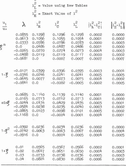
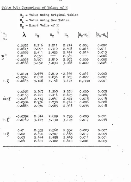
The fitting of the functions is carried out in chapter three. Polynomial models in terms of

A

are fitted by least squares tech­ niques to data from seven solutions and are adjusted to ensure an analytic form for H for small values of A » A comparison of results using new and old tables indicates that an improvement has been made

The transformation relating certain compressible and incom­ pressible flows is next examined and the extension of the method to such problems considered. An idea due to Stewartson for assessing the relative accuracies of methods under such circumstances indicate;

that the method should be highly accurate, a result confirmed by the calculation of the compressible flow u.^ = Uo(l-J) at a leading edge Mach number of four.

I should like to express my thanks to my super­ visor, Professor S. N. Curie, for his guidance and encouragement during the work contained in this thesis, to Mrs. Cunningham for her preparation of the typescript, and to Mr. McQueen for carrying out the printing of

this thesis.

CHAPTER 1 ; INTRODUCTION

Section I: Introductory remarks

Section II : Derivation of, and background to the method

Section III : Critical assessment of the problem

CHAPTER 2: THE PROBLEMS u,, = V L o ( f + ^ ^ ) AND u = Uo(l+^)

Section II: Collection of data

Section III: The fitting of the forms

Page

1

7

20

Section 1: Introduction ₃₃

Section 11: Initial series expansions 34

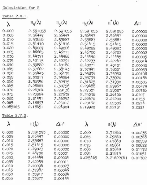
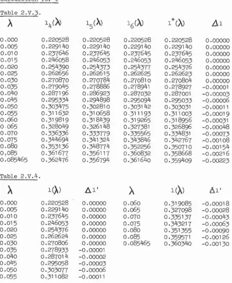
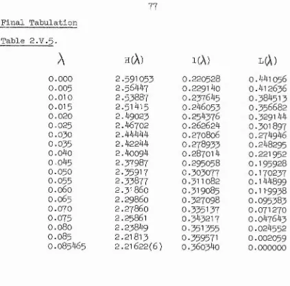
Section 111: Asymptotic theory for u^ = Uo(|’+^^) 4o Section IV: Calculation of the quantities H, 1, L

as functions of X 56

Section V: Calculation of the parameters H, 1, L.^and

\i for the flow u.^ = Uo(l+J) 68 Section VI: Runge-Kutta techniques applied to the

solution of the momentum integral equation for the cases u = Uo(jS+€^)

and u^ = Uo(1+^) 78

Section VII: A new series expansion for displacement

thickness ₈₃

"TER 3: ATTEMPTS AT IMPROVING THE TABULATED FUNCTIONS Po(X). Go(X), PpA) AND apA)

Section I: Introductory remarks 88

89

CHAPTER 4: THE APPROACH FOR TFIE COMPRESSIBLE LAMINAR BOUNDARY LAYER

Section I ; Introduction

Section II: The Stewartson-Illingworth transfor­ mation

Section III: An idea due to Stewartson for assessing the relative accuracies of approxi­ mate methods

125

127

130 Section IV;

Section V:

The extension of Stewartson’s analysis to the Curie two parameter method with special reference to its appli­ cation to the compressible flow with external velocity u^ - Uo(l-^)

The extension of Stewartson's analysis to further compressible flows

CHAPTER 5: CONCLUDING REMARKS

APPENDIX: DOME'S RATIO TEST

REFERENCES :

137

147

152

157

u = component of velocity within boundary layer parallel to surface

V = component of velocity within boundary layer perpendicular to surface

X = co-ordinate along surface

y = co-ordinate perpendicular to surface

c = length characteristic of distance parallel to surface 5 - length characteristic of distance perpendicular to

surface

u^ = external velocity at the edge of the boundary layer V = coefficient of kinematic viscosity

Cbapter I - Section I: Introductory Remarks

The work of this thesis Is concerned with the investigation and attempted improvement of a practical method for solving the steady,

two dimensional incompressible laminar boundary layer equations of fluid dynamics. For the purposes of this thesis it will be assumed that the boundary layer forms at a fixed impermeable surface so that, in the usual notation, the underlying problem is to solve the equations of con­

tinuity and momentum which are

t * ’ ê ""i <s'

respectively, subject to the boundary conditions

u(x,0) =: v(x,0) = 0; u(x,y) -> u^ (x) as y oO ,

For many years the solution of these equations for a general external velocity distribution u.(x) has proved to be a very difficult problem and only with a good deal of trouble have solutions for the simplest forms for u^(x), been found. It has therefore been necessary to develop methods which solve these equations (or suitably transformed versions) approximately, the nature of the approximation coming sometimes from physical insight, and sometimes from mathematical intuition. Many such methods have been developed possessing varying degrees of accuracy, reliability and ease of application. This thesis is concerned with the investigation of one of these methods, a method based on a sound

computer and the resulting development of the techniques of numerical analysis have helped to make the problem of solving the basic equations

1 o

more tractable (a recent review article by Smith outlines some

of the better methods). This, in its turn, has raised the question as to whether there is still any need for the approximate method. Pro­ vided we think of the roles of the approximate method (which may well make use of a computer) and the ’computer’ method as complementary, the answer to this is yes.

When what we want is a method of calculating the downstream development of quantities such as the skin friction, t , (especially

important since it vanishes at separation) the displacement thickness 6^ and the momentum thickness Ô it is convenient first to find an

equation which relates these directly. Such an equation is simply obtained by integrating the momentum equation across the layer and substituting from the continuity equation to eliminate the normal component of velocity. The equation so obtained is called the momentum integral equation and is

p “ dx (^^ 2) "1 dx 1

.

On defining a pressure gradient parameter /\ - u ’ — , a shape parameter

0 0 I V

H = — , a skin friction parameter 1 = and L = 2 .'1 (H+2) 1 the

2 ^ L,

above equation may be rewritten as

b / A \ _ L dx^u' ” u^

directly to yield a simple formula for the momentum thickness 6g in terms of the external velocity distribution u^(x). With this approxi­ mation and tables of the parameters H and 1 versus compiled using the known solutions, he produced a method, easy to apply and of con­ siderable accuracy.

The method of Thwaites was further refined by Curie ^ who

showed theoretically that a more accurate two parameter representation of L and 1^ is

L = Po(A) - m-Go(A)

and = p y A) - (A) 2 u u”

where p = ^ 1 1 . A careful examination of the then available range K f

of known solutions enabled the four functions Fo, Go. F^ and G^ to be tabulated against \ . With these tables the method of Curie, described in some detail later in this chapter, produced answers to the standard problems of incompressible boundary layer theory in even better agree­ ment with the exact solutions, than those given by the method of Thwaites

has been available for an accurate determination of these tables. To remedy this, solutions to the Incompressible flows with external

velocity distributions u^ - Uo(14-^) and u^ = with , (which cover the ranges over which insufficient data was available) have been calculated and the methods used and data calculated are presented in Chapter II. It is also found that the methods used for fitting the data may also be improved. In the third chapter these techniques are investigated and the new tables produced using better fitting techniques on a wider range of data.

Another problem which is tackled in Chapter IV is the extension of the approximate method to the solution of certain compressible boun­ dary layer problems which may be transformed into associated incom­ pressible flows. It is shown that these transformed flows often behave in a manner for which the standard approximate methods of boundary

layer calculation are inapplicable and yield widely inaccurate results. For one such compressible flow for which an exact solution is known the calculation using the Curie approximate method is carried out. The

result obtained is found to be in good agreement with the exact solution which indicates that the new method has a wider range of application

than many of the existing ones.

in the method and on the accuracy of which the method relies. An added aim is to make the method applicable to certain types of compressible boundary layer problems and generally to improve on the range of

Section II; Derivation of and Background to the Method II.1 The Governing Equations

For clarity I shall derive or quote now certain forms of the equations on which the method is based. The boundary layer equations for steady, two-dimensional incompressible flow may be written, in the usual notation, as

0 )

After integrating equation (2) with respect to y from y = 0 to y =, we obtain the momentum integral equation, for zero transverse

velocity at a solid surface.

T du

“ = é ( 4 g ) + "1 ar' H (3) This equation expresses conservation of momentum as a whole and may be written alternatively as

s

<i; > -

_s,

_Cl

\ ^2 ,

where A ~ ^ ^ pressure gradient parameter, 5 2

^ ~ u ^l^^w * ^ skin friction parameter,

H = — , a shape parameter, and 2

A further useful integral form of the boundary layer equation may be obtained by first multiplying equation (2) through by u and then integrating from y = 0 to y = ^ , This gives

and expresses the physical fact that the rate of change of the flux of kinetic energy defect within the boundary layer is equal to the rate at which kinetic energy is dissipated by viscosity and will be referred to as the kinetic-energy integral equation. Equation (5) may be rewritten as

& ("lb) = X (6 )

where D = dy

5-, 6gD

By Introducing the non-dimensional quantities H, = — ; D, = ---_ ^2 ’

equation (6 ) may be rewritten as

^ (7)

%

If we now multiply through equation (7) by 2u _{1 1 2} and integrate we 6., 2_ 2 „ r

obtain u^

or 62 = ^ I H^D^u^^dx (8)

H-j 'J§

to y , V can be eliminated provided that P(g^) is an exact differential coefficient of u and its derivatives. It is therefore

clear that two families of possibilities are P -Ou m ^^u

and P = (ys-^) . The cases n ~ 0 and n = 1 correspond to the

momentum and kinetic energy integral equations respectively. It will be seen at a later stage how use is made of these forms and how the

3u m

other family P = (g-) (—-g) also contributes useful integral forms, II.2 The Background to, and Development of the Method

For many years after _Prandtl introduced the concept of the boundary layer the number of accurate solutions to the equations which governed its behaviour even in the simplest case of steady, two-dimensional incompressible flow were few. Of these few solutions there were two types, which will be referred to later as the 'exact* or 'special' solutions.

The first type was for those flows where the geometrical pic­ ture is very simple, such as the problem of flow past a flat plate held parallel to the stream, or where the domain considered is very limited, for example, flow sufficiently near to the stagnation’point of a bluff body where the body may in effect be regarded as a plane normal to the stream. In these cases, appropriate transformations could be made to reduce the boundary layer equations to a single ordinary differential equation, the solution of this equation could then in theory be obtained to any required accuracy,

The second type of solution arose when the shape of the body is assumed such that the external velocity u.(x) may be taken as a

power series in x containing say, two or three terms. In these cases, the velocity u in the boundary layer may be expanded as a

power series in x, the coefficients being functions of say y/o, where b Is representative of the scale normal to the surface. These

functions are obtained by solution of the appropriate sequence of ordinary differential equations of which all but the first are linear.

To obtain solutions by these methods, even for the simplest cases took a considerable amount of time and effort and attempted an accuracy which was often unnecessary for practical purposes. Much research time was therefore devoted to constructing methods which would be quicker to apply and would give acceptable if perhaps slightly less accurate solutions.

Many of the first approximate methods were based on an idea

due to Pohlhausen It consisted in making some plausible assumption .about the general shape of the velocity profile within the layer. In the simplest form of the method the velocity profile was taken to be a function of the non-dimensional co-ordinate normal to the wall % = y/b, where b is a length characteristic of the thickness of the

fcrm of the momentum integral equation now contained quantities which could be tabulated numerically using the results from the 'special* solutions mentioned earlier. Given these tables the momentum inte­ gral equation could be integrated to yield the required quantities

6^, bg and The choice of the form of the approximate velocity profile and of the boundary conditions which it was made to satisfy was rather arbitrary, and often a point of contention. Pohlhausen*s particular choice of velocity profile was

a. + V i +

the coefficients being chosen to satisfy the conditions

'" = 0- = - V to ' "hen y = 0

"u _ g b

'' «y

and u = u. , _{Ù Y} = 0, ^ = 0 when y ~ b_{% 2}

The method appeared in general to give good results in regions of favourable pressure gradients but was somewhat inaccurate as regards the prediction of separation. Various attempts were made to improve the method. For example, Howarth^^, based his velocity profile on the solution to the problem with external flow u.^ = Uo(l - -g), Walz^8

profile and dependence was assumed solely on the non-dimensional normal co-ordinate. This, in turn, meant dependence on the one parameter

A

ôo^ du4

= -ÿ— , which makes its appearance through the condition that the momentum equation should be satisfied at the wall.

The approach of replacing the velocity profile by some poly­ nomial approximation was regarded as the most satisfactory practical

2*5

approach until Thwaites pointed out that if what was required was the calculation of 5^ ^ bg and then a detailed knowledge of the velocity profile within the layer was not necessary but rather all that was required was a suitable correlation between the boundary layer properties H, 1, L and A <- He found that though there was some variation in the curves of H and IvA from solution to solution,

especially for negative \ (i.e. in regions of unfavourable pressure gradients) the variations of L(A) were less pronounced and that L(A) could be taken as roughly linear for all solutions. He found that choosing L(A) = 0.45 - 6A gave good agreement with all the known solutions and with this form for L(A) equation (4) could be integrated to yield a formula for 6 in terms of x

bg - 0.45Vu.^ ^ I u^^dx (9 )

known, by making use of the tabulated values of 1, the skin friction T could be obtained, and using the tabulated value of H the dis­

placement thickness 6- could be obtained. The position of separation

• . I

of the boundary layer which is taken to be where = 0, was cal­

culated by finding the value of x which gave the A such that

1(A)

~ 0.

For Thwaites* method it is assumed that 1(A) = 0 when A “ -0.090. This method, essentially empirical, reproduced the known * exact* solutions to a reasonable accuracy and with its ease of application

was widely accepted as one of the better practical methods. It was

shown in an even better light when Leibenson ^ ^ and Truckenbrodt^^

showed that by making simple approximations in the kinetic energy

integral equation Thwaites* fitting of L as a linear function of A could be justified. They pointed out that and were approxi­

mately constant over a wide range of pressure gradients. The approxi­ mate constancy of could be traced to the fact that it is the

ratio of two integrals, each of which has an integrand which is zero at the wall. Now if we compare the velocity profiles at. various stations, they will differ greatly between stagnation point and

separation. But upon closer examination it is found that the slopes

of the outer parts of these layers do not differ much and that the

greatest changes of profile shape occur in the region close to the

wall, where the velocity is small and little contribution is made

to either of the integrals for 6. and _{2 3} Thus H. = — might be_{I Og} expected to vary but little, even though the velocity profile varies

a lot. The argument for the constancy of is that the decrease in the contribution to the dissipation integral as the skin friction

decreases to zero at separation is partially balanced by an increase

in momentum thickness and a decrease in the local mainstream velocity. On making the assumption that and were constant equation (®)

reduced to D

= | u i 5 d x (10)

The values chosen for and were = 1 .57, = 0.172 which were the values for a Blasius layer. These values as well as being

rough means,, are also particularly accurate in the region close to

a pressure minimum where the integrand in (8) has a peak.

With these values of D- and H- equation (10) becomes

2 ^ 1,1, - _{= O.Hl VuV'^} -6 _{dx (11)}

and L = 0.441 - 6

/^,

very close to Thwaites' formula. The methods

considered up to this stage have the one major drawback that they all

assume dependence only on the one parameterX• Tani^^, pointed

out that A does n6t exactly fix the velocity distribution and that

the boundary layer characteristics especially near separation are

unlikely to depend solely on the parameter X • He mentioned that

\ 2 2

other parameters such as p - A u^u^"/(u^') also affect the distri­ bution, the influence becoming more marked as separation is approached.

Tani did not however construct an approximate method which made use

/ I p

a lot. The argument for the constancy of is that the increase in the contribution to the dissipation integral as the skin friction decreases to zero at separation is partially balanced by an increase in momentum thickness and a decrease in the local mainstream velocity. On making the assumption that and were constant equation (4)

reduced to D

0/ = r I u 5 (10)

1 -4

The values chosen for and were = 1 D-| - which were the values for a Biaslus layer. These values as well as being rough means, are also particularly accurate in the region close to a pressure minimum where the integrand in (4) has a peak.

With these values of and equation (IO) becomes

5g = 0.441 f’u^" I dx (11)

and L - 0.441 - 6^^ very close to Thwaites' formula. The methods considered up to this stage have the one major drawback that they all assume dependence only on the one parameterX. Tani^', pointed

out that A does not exactly fix the velocity distribution and that the boundary layer characteristics especially near separation are unlikely to depend solely on the parameter \ . He mentioned that

2

other parameters such as p - ) u^u^"/(u^')^ also affect the distri­ bution, the influence becoming more marked as separation is approached Tani did not however construct an approximate method which made use

p

see how this new parameter, p, mentioned by Tani, was put to use.

What Curie did was as follows. In equation (8 ) instead of making the assumption that = const, =% const he made the small correction ~ . After differentiating this

equation with respect to x and re-arranging he deduced that

+ 6i = 4 -gi - 2 A ^ . ~

(12)

and by equation (4) this yields

V D u dH

L 4 6A = 4 g- - (13)

But

On substituting this form into (13) we obtain

b xt' f \ "i4' I

= 4 - - 2 A g ^ | l 4 A - ^ 2 | ('5)

I- H

o r

Î \ H' ■) B H;

5----6X “ 2p — (l6 )

where

h = X (17)

Equation (l6) can be written in the form

L = Fo(A) - 14Go(A) (18)

where 4d - 6 ^ 2H'

Fo(A) = + 2A'h ' ’ “ H ~ T 2 ^

Primes denote derivatives with respect to A . except in the case of

E l Lieu ( l 8 ) gives a convenient form for L and Involves the parameter \i which had been mentioned by Tani. The problem now reduces to trying

to find universal forms for i 'o(A) and G o (A) and also to trying to

determine whether it is possible to express 1 in a similar form. With the solutions then at his disposal (u.^ = Uu^^, = Uo(l - ^ ,

~ Uo sinj^ and u.^ = Uo(l “ J^)) Curie made a careful examination

\

of the sets ( L , , p) to see whether it was possible to determine a function Go (A) such that the results I, + pGc(A) when plotted against

Xall fall on to one curve. After a certain amount of intelligent trial and error Go(X) was chosen such that Go (A ) - 0.66 -f . The

new values of L were then given by = EoCA) - pGoQ) wh.n-e

Po(X) and Go (A) could be tabulated once and for all. Once the value

of L(A^p) is determined, the momentum thickness 5 (x) is given by the solution of the equation

d

u._{1 dx 'V}(\f) “ L(A,p) =F„(A) - iiGc(A) (19)

A simple method of solution of this equation is by iteration. Thus we write

Po(A) - uGo(A) =0.49 - 6> 4 g(yi.i) (20)

where the term g(A*p) defined by the above equation is the correction

to the Thwaites’ formula. Since

g ( A p ) Fo(A) 0.45 ) 6/i - pG^(/|) (21 )

^1 Ac ("y ) = 0.45 + g(X^M-)

which may be formally integrated to give

&2 = 0.45\Tu^" f (1 + 2.22g) ax (22)

For a first approximation g(Xp) is set equal to zero, and once the corresponding values of and p have been determined, these are used to estimate g(X^H) for a second approximation and so on.

To express 1 in a similar form was a more difficult task and led Curie to look for new integral forms of the boundary layer equations. Further members of the family P = u^ produced no more useful

relation-2

ships and it was to the family P = that he next turned. The first member m = 0, yielded the form

f* /P,2 2

^ ^

^ (23)

There are two reasons why this equation (25) did not produce a suit­ able form for the skin friction parameter 1, and, following the

2

arguments of Curie , they are.

In the above equation (25) it would be convenient to write

u (|H)2 B = ^

layer and a typical separation profile, indicated that the values of B varied by factors of up to 5 or 4 and A by factors of up to 8 or 9, so A and B are far from constant.

Secondly, it is well known that the various curves of 1 against \ drop sharply to zero as separation is approached, because of the singularity in the boundary layer equations which almost certainly exists at that point. This singularity in the boundary layer

equations at separation shows up as a square root singularity in 1. In view of the fact that these sharp falls in the values of 1 occur at different values of X it is difficult to see how the curves of 1 against \ can be collapsed on to a single curve.

For these reasons equation (23) had to be discarded. The next member with m = 1 yielded the

form:-_d_

dx

(

#4 -

dy

(24)

2 ^

This is an equation for 1 and since the singularity in 1 is square-root in nature, the curves of 1^ against X a.re well-behaved even close to separation. On examination of the quantities

2 4 r**

So I •a,, 3 SZ f « g2 2

-Tf I u(gp) dy. D=-^ j 0^ (»-#) dy

(25)

c

it was found that they were approximately constant. Substitution of the forms of equation (25) into (24) yields

u u

dl (C Yg) = -:2— 1 (26)

In this equation we note that by setting C - const, D = const we retrieve the Thwaites' condition which is 1 = 1(A) • For separation this becomes 1(A) = 0. If we then take C = C(A) and D = D(-V this yields the improved formula

F = f/A) - (28)

where F^

(A)

and

(A)

are rather complicated functions of G and D. The search for a function G^(A) to make the results of 1^ + pG.

(A)

when plotted against A fall on to a single curve for all solutions was carried out in a manner similar to that for Go (A)« The resulting

function G^

(A)

was given as a numerical tabulation. The separation condition becomes

0 = F^ { A ) - UG.^

The method of completing a calculation of the usual boundary layer characteristics is now quite straightforward. Having determined A and bp as functions of x, as described earlier, the values of 1 and hence are given by equation (28). Equation (20) may be used to determine H, whence 5^ = Hôp follows.

Section III: Critical Assessment of the Problem 111.1 Introduction

In the previous section the method was derived and set against the background of boundary layer theory. In this section a discussion is given of some of the ideas behind the construction of an approxi­ mate method based on integral forms of the boundary layer equation

and these ideas are illustrated with reference to the Curie 2-parameter method. This discussion indicates certain points which may require further investigation. Later in the section an outline is given as to how these points may be tackled. Finally in this section an indication is given as to how the method may be extended to certain compressible boundary layer problems. An outline is given of some of the analysis from which it may be seen for what types of problem the method may be expected to give good results.

111.2 Pinpointing the Problems

ideas are complementary and the difference in approach may be seen by comparing the derivation of the Thwaites' method and the Curie 2- parameter method,

Thwaites examined the curves L versus X from all solutions (then available) and decided to fit the form L = a + bX to these points.

This was later justified by the work of Leibenson*'^ and Truckenbodt^"^ who, as described earlier, showed that Thwaites* empirical form

amounted to taking ~ const, = const in the non-dimensional form of the kinetic energy integral equation. On the other hand Curie first

shows that taking H, = H^(X), (X) yields a better 'between solutions’ representation for L in the form

L = Po(X) - pGo(X) where p = \2 ^1^1 ' (u;)2

and that a similar type of approximation and more complicated inte­ grated form of the boundary layer equation yields the form

F = ppA) - u g/A)

He next proceeds to examine the available data in the light of these forms and tries to extract universal forms for Fo(A)^ Go(X), F^ (X)^

G^ (X) to give good agreement for L and 1^ with all solutions. At this point we can see over what range the method may be expected to work. Our underlying forms depend on the two parameters X and

p = A ----^ . The range of the method is therefore determined by the (q

The more solutions available over a particular range the more confident we can be that we can choose the universal functions to describe what is actually happening and remove any bias towards one solution or another. If we examine those solutions on which the current Curie tables are based we may see where an improvement may be made. At the time that the tables were derived Curie had at his disposal the

î*i 2

following exact solutions u^ = Uo(l - - Uo^ , u^ = Uo(l ), u^ = UoSin^ . From an examination of the values ofX which these solutions yield it is seen that they are heavily weighted towards the negative end of the range. The tables constructed from these solutions are reliable for the range of X which these solutions cover. However for problems which yield values of A outside the range of X covered by these solutions the tables possibly give less accurate results, with greatest possibility of inaccuracy being in the range^ > 0.0685

(beyond Terrill's solution for u^ = UoSinf ) where the only solution used is u^ = Uo^ To remedy this two new exact solutions were found corresponding to flows with external velocities u^ = Uo(J ) and u^ = Uo(l ), The first solution yields data for 0.0855^

X

^ 0.0984

and the second for 0.0 ^ A ^ 0.0855» The techniques used for these problems are outlined in the next section and dealt with at greater length in Chapter 2.

We next have to consider how we estimate the accuracy of an

method and the agreement between the ’approximate' and 'exact'

solution examined. The better the agreement, the better the method is. In terms of the Curie method the accuracy therefore depends on

2

how closely L and 1 reproduce the known data. This in turn depends on how accurately we can determine the functions P o ( A ) : . G o ( A ) , ( A )

and G^(A). As was described previously what Curie did was to examine a few solutions and on choosing Go( A ) - 0,66 + 3A found that the cal­

culated values of L + pGo( A ) foil almost on to one curve when plotted

against A » This curve was smoothed and the smoothed values were

chosen as Fo(A)o A similar analysis was performed for 1^ but there was no obvious linear form for G.( A ) which reduced all the solutions

1 ^ + pG^( A ) to the one curve. However G^ could be found as a numeri­

cal tabulation versus A to make 1 ^ + pG^( A ) fall almost on to a smooth

curve, and these values could be taken for P ^ ( A ) , An attempt has

been made to improve the values of these numerical tables, as will be described later, mainly by using techniques of least squares curve fitting on a function of two variables.

Another problem arises in the determination of the function H. Once the functions Po(A)^ Go (A), F^ (A) and G. (A) have been tabulated then, given any external velocity u,(^) we can determine A and p and

2

so obtain L and 1 , H is then given from the relationship

L = 2^1 - A ( F + 2)^ i.e. H = - 2. For small values of A ^ H

2

analytic form for H was derived which would be valid for small A «

To conclude this section and lead on to the next we may say that there are two broad areas in which a further investigation of Curie's two parameter method may be profitable.

(1) In extending the range over which the method may be applied with some reliability.

(2) In improving the existing tables by a better fitting of the data, and in the region of small A producing an analytic form for H.

III.3 Extending the Range

As described in the previous section a possible improvement to the method could be to add in more solutions, for the derivation of the tables, for positive values of A» This has been done by investigating and deriving accurate solutions for the two problems u^ - Uo

and u^ =! Uo(l )» An outline of the methods used (principally in

connection with the flow u^ = Uo(^ + J'^)) is given below and the details are given in Chapter 2.

Initially it was hoped to use methods similar to those used by Curie in his treatment of the flow with external velocity u^ = Uo(ÿ -Briefly what this involves is as follows.

When the external velocity is given as a power series i n V , a formal solution of the boundary layer equations may be obtained by expanding the stream function as a power series whose coefficients are functions of the distance normal to the wall. Thus for a main stream

f = Ln+1 where/>^= (U) a. 1

^ y

It has been shown by Howarth that the functions (^yj) may be

expressed as linear combinations of a sequence of universal functions, which can be solved and tabulated once and for all. Once these uni­ versal functions have been tabulated the solution of any boundary layer problem with an external velocity of the above form can be reduced to the arithmetic of these functions.

It follows by differentiation that the velocity u in the boundary

layer is oo

o

and that the skin friction at the wall is derived from

^ A

0

Using the definitions,similar series expansions may be derived for and bg.

One drawback of this type of method is that it is difficult to calculate any more than the first few terms of the series expansions Involved and often these fail to converge except for very small

values of ^ . Following an idea of Howarth^Curie made the following assumptions about the series expansions.

(a) Assume that the convergence of the series is such that the seventh and subsequent terms may be treated as a relatively small correction to the first six. The validity of this is examined a posteriori.

may be adequately estimated by assuming that the n ^ 6, are similar in shape to -j

%

On the basis of these approximations we may write the velocity as

' 0

and the skin friction as

T = (ϧE (|)„ ^2n+1 (°) + pyo) *

0

where A(^) is to be determined.

Using a differentiated form of the momentum equation evaluated at the wall this approximation enables the calculation of the skin friction

(t) to be reduced to the solution of the simple, non-linear ordinary

differential equation

where P is a known polynomial, determined from a knowledge of the mainstream velocity. Once T has been obtained, the relevant value of A(^) is deduced from (-^ ) by subtracting off the series expansion terms.

The displacement thickness is obtained using

(u^ - u)dy and yields. In terms of A(^) Oq

1 _ 11m J 3 YC» 2n+l

(a^Vc)^I»,

/ F '

2

J

'

1

' -

f

The momentum thickness S. is obtained by the solution of the momentum inte­ gral equation using the expansions for and 6^ .

since separation occurred for^ = 0 .655» covered only small values of ^ . For the flow u^ = U o t h e assumption (a) is violated onceÇ % 0.5 and so the method is of limited usefulness. Up to this point it does however give a highly accurate prediction of what happens and so its use may be justified in giving the initial development of the solution.

Originally it was hoped that the above technique would give the develop­ ment of the boundary layer to larger values of^ than it was found to do. It was hoped that these values could then be matched in with an asymptotic theory which was developed as follows.

For large ^ J ^ and it is assumed that the velocity within the layer will behave only slightly differently from the corres­ ponding Falkner-Skan solution for the external flow u^ = UoJ" Since the behaviour of these solutions is well known it was thought that it might be useful to work out the development of the solution for large

values of^ in terms of a perturbation to the Falkner-Skan solution for the flow u^ = UoÇ ^ , This was done by defining the stream function (5

for the flow with external velocity u^ = U o t o be of the form

where ^ ^ ^ and f satisfies the equation

in the expansion was solved. Though, in the event, this analysis was not used to produce the relevant parameters, it gave an interesting Insight into their asymptotic behaviour.

The approach to the problem which did provide satisfactory answers was as follows. For both of the flows under discussion it was observed

from the work of others, that in the range of interest of H, 1 and L were almost linear functions of A » It was therefore decided to try to express H, 1 and L as functions of A , in the hope that these new forms would give, to a reasonable accuracy, the correct limiting values corres­ ponding to limiting values of A » This was done by first expressing A^ H, 1 and L as functions of^ and then eliminatingÇ between A ^nd H, /\ and 1 and A 9.nd L to give H ( A ) ^ 1 ( A ) and L ( A ) » The series expansions which

resulted gave good agreement with the known limiting values and only needed the addition of small correction terms.

For the problem u^ = Uo(l ) this is the only approach discussed. Once L had been calculated as a function of A an attempt was made. In each case, to solve the momentum integral equation by a Runge-Kutta type method. Some success was obtained with this method over the whole range of Ç for the problem u^ = Uo(1 + ^ ), but unfortunately little success was met with for the flow u^ = Uo(^+t^).

section of chapter two.

Ill 04 Improving the Accuracy

III.4.1 Collection of Data

To improve the accuracy of the tables, the solutions used in cal­ culating the original tables were found to a greater number of figures and

2

then the forms for L and 1 fitted to these by means of least squares. The solutions used were as follows.

A. The Falkner-Skan Solutions. u^ = Uo^^, ^ —

6

The values used were those due to Evans , plus a few of the original

o

Hartree values.

B. The Howarth Solution, u. = Uo(l - P ). ? = —_{■■■■ I --i / — 0}

The original Howarth solution/^ for this flow was tabulated to more figures to allow for rounding errors.

C . Tani' s solution. u^ = Uo(1 - ^

Professor Tani very kindly supplied an improved version of the table of values (appearing on page 96, Chapter 3) with the new values tabu­

lated to four significant figures. D. P. G. Williams solution

with the compressible flow with external velocity distribution u^ = Uo(l-J), zero heat transfer at the wall, Prandtl number cT" = unity, the viscosity \i proportional to the absolute temperature T and Mach number at the leading edge being equal to 4. P. G. Williams of University College, London supplied me with details of his solution to this problem from which the relevant

parameters could be calculated.

E and F The flows u^ = Uo(^-^^) and u^ = Uo ( 1

An outline of the methods used has been given in the previous section and these will be given in more detail in Chapter II.

G. Terrill's solution, u^ - UoSin^

The required parameters were calculated from data given in Terrill' paper, (reference 22).

111.4.2 Fitting of the Data

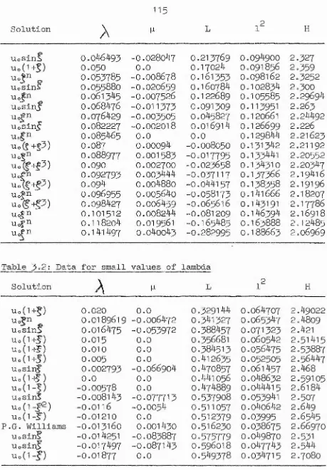
Once values of the parameters from the solutions mentioned in the previous section had been calculated, from these a set of sixty-two points was chosen covering the range -0.1167^ 0.14l and also representing all the solutions.

Since the initial approximation for Go(A) was linear in A it was

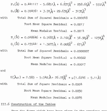
decided to attempt to fit the functions Fo, Go, F^ and G^ as polynomials in A? over the whole range. It was found that a convenient and flexible method of fitting these forms was to take the models as

L = ao + a^X + a^A + . a + bop + b^ p/\ + ... b^pA^ 1 = Co + c^X + ₁ c + dop + .... d pA^_{q pt}

L = &o ■'* a. X- + a^X^ • • • a X + boYo + ♦ • » b Y_{1 1 2 2 n n r r}

= Oo + o,Xi ₁₁ o X + doYo _{q q} d Y_{p p} 2

by defining X^ = Xg = \ ' e t c . Yo - [ i X ^ Y^ = [ x X \ etc.

and then use the IBM Scientific Subroutine package REGRE which Is used in multiple linear regression. The functions Fo (X) j, Go (A), F^ (A) and G^ (A)

could then be determined from

Fo(A) =<■' a X : G.CX) = - V b Y

k I .21— I

r=0 r—0

r=0 ri)

where the negative sign is taken in G o ( A ) a-^^d G^ (\) to give agreement with the

approximations, originally used, L = F o ( A ) - p G o ( A ) and 1^ = F^ ( A ) - p G ^ ( A ) .

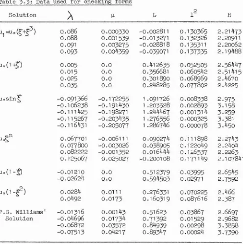
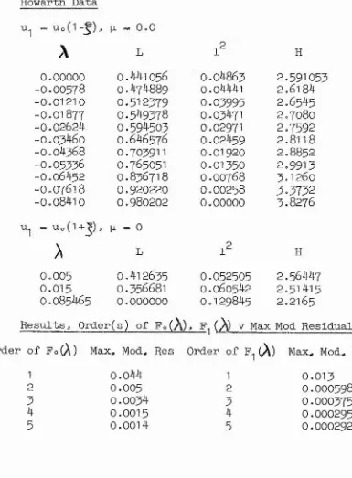
From an examination of the flows u^ = Uo(l-Ç) and u^ = uo(l+Ç*) for which p = 0, some idea as to the orders of polynomial approximation for F o ( A ) and F,^ (A )

was found so that a certain amount of the work in fitting these functions over the whole range could be cut down. For comparison of models the residual

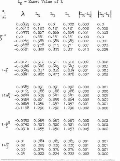
sum of squares, mean modulus residual and root mean square residual in each case were calculated. Once forms had been decided upon from use of the sixty- two points, these forms were tested by calculating the above-mentioned resi­ dual quantities at twenty-five points which had not been used in the fitting.

For small values of A ^ -0.020 <'A'^ 0.020, a similar separate analysis was carried out with the added restriction that the leading coefficients in

2 2

the forms for L and 1 should be related such that C o = a.o/4 and d o = a o b o / 2

to ensure that H would be continuous for A == 0. For A in this range the

From these forms a tabulation of numerical values of these functions was compiled. These tables and the methods used to obtain them are described in greater detail in Chapter III.

III.5 Extension to certain compressible boundary layer problems

It has been shown independently by Illingworth^^ and Stewartson^^

that a compressible laminar boundary layer problem can be reduced exactly to an associated Incompressible problem subject to the following conditions: a) there is zero heat transfer at the wall

b) the Prandtl number O'" is unity

c) the viscosity p is assumed to be directly proportional to the absolute temperature T .

However the transformed flow, especially at higher Mach numbers, is often very different from any of the flows for which existing methods produce good results. It was therefore thought to be useful to examine certain

CHAPTER 2: The problems - Uo(§ and - U o (1 = -g

Section I: Introduction

This chapter deals in greater detail with some of the ideas outlined in Section III of Chapter 1 for solving the problems u^ = Uo

and u^ = Uo(l ) » Most of the analysis was carried out for the problem u^ = UoG> +5^) and this problem will therefore be given more attention than the problem u^ ~ Uo(l ) for which only that method which did produce the eventual results is quoted.

The next section deals with the Howarth-Blasius series approach to solving u^ “ and with Curie's idea for extrapolating the values of the skin friction. Though it had been hoped that this approach could be extended to higher values of ^ than it was event­ ually found to do, the analysis is produced as a highly accurate initial development of the flow.

The third section deals with the asymptotic theory for large values of^ when Uo u^^, and the velocity within the layer is assumed to be only slightly different from the Palkner-Skan

solution. An analysis is carried out to find the form of the co-ordinate perturbation expansion from the Palkner-Skan solution and the equation governing the first term in this series is solved. With these forms the asymptotic behaviour of the parameters can be

The fourth section describes the analysis which did provide satisfactory results. It involves the calculation of the parameters Hj 1, L A functions o f ^ and then the elimination o f ^ to give H(A), 1 ( A ) » L ( A ). These expansions required only slight adjustment

to give the correct asymptotic form.

In section five, the successful techniques are described for the flow u^ = Uo(1 4-^ ) and section six deals with the application

of Runge-Kutta type methods to the solution of the momentum integral equation once L has been given as a function of A »

The seventh and final section contains some interesting analysis of some series expansions which have arisen in connection with the non-dimensional displacement thicknesses for the flows u, = Uo(^ ^) and u^ = Uo ( I ). It has been found that the relevant series

expansions, slowly convergent in terms of Howarth-Blasius variables can be made to converge much more quickly when recast in terms of a new variable which is found by using a suitably chosen Euler trans­ formation.

Section II : Initial Series Expansions

As has been described in Chapter 1, where the mainstream velocity u^ , may be expressed in the form

oo,

^ 2n+1 p X , .

° / , ^2n+lS ' f = c (2.1 )

1

'=-■ Tn+l (2.2)

0

where the coefficients are functions of the scaled co-ordinate a 1

^ y 3 normal to the wall. These functions, des­ cribed previously, may be expressed as linear multiples of certain universal functions (Howarth9) which have been calculated by various workers. The velocity within the boundary layer, u, and the

non-\7 % d

dimensional skin friction T = ^^e then given by a

o o

u ^S^Lsn+l

w

a., q;

0

and T

The coefficients of all terms up to and includingj; have been cal­ culated and, for small values of P , the small contribution of sub­ sequent terms may be evaluated by assuming that their dependence upon 4^ is similar to that of the coefficient of \ That this will often

be a reasonable assumption may be concluded from the work of Howarth^^, who in considering the flow u.j = Uo(1 ) found that the coefficients

of^ were remarkably similar in shape when n = 5>6,7,8. The equations (2 .3 ) and (2.4) then become

^ = S " " " ' (%) + "(|^ 4(%) (2.5)

and T + Ag") F^O) (2.6)

Q

on a differentiated form of the momentum equation the following equation is obtained for T

where P = (2‘8)

O Y

and (0) - 0 1 (O) (2.9)

Equation (2.7) may be integrated to give

where

.-j_j -u

2n4l ^ 2n+2

Q ( | ) = 2 Pdj = 3 2n+2 (2.11)

/ ₄1

o

Equation (2.1o) may then be solved by a procedure due to Thwaites^ , r

(1949), in which | TdÇ is replaced by its Simpson's rule equivalent. Jo

Hence if ) and T(^+ h) are known, the value of T(^ + 2h) may be determined by solution of a quadratic equation. Having obtained T, the relevant value of A(^“) is deduced from (2.6) by subtracting off the first five terms and dividing by Efj(o). The non-dimensional dis­ placement thickness is given by

r 4,

"1 ^ llm * "

(aye) 2 I A t ^2n+1 (%) - "(p (2-12)

The momentum thickness 6^ can be obtained, using the values of skin friction and displacement thickness, by solving the momentum integral equation.

- Uo, = a^ = ... =0. Therefore using the same notation as Curie we have

= f^j P^ = 4f^j P^ = 6h ; = 8k^; F^ = lOq^; F^-j ~ 12n^.p

This yields the first six terms in the series for the non-dimensional skin-friction as

T = f,«(oÇ + k t ' ^ Ç o ) f ' + 6h^(0%r5 + + 10q^(0)ç9 + 12n!J(0^11 ^

= 1 .2 3 2 5 8 ^ +

2

.

8977

^ ^ + 0 .7 1 5 0 9 Z + 0.061 nç'"^ - 0 .3 0 7 ^ ^ + 0.6187^11 ^ (2 .1 3 )

using the values as given by Tifford^5

The corresponding expansions for and 6^ are

(H£) 1 6 = 0-6479^ -0.1 13896^ ^ +0.4434^:5-0.79612^^+1 .3967^ - 2.4 9 0^

-I-T + i )

and

0 .2 9 2 3 4 4 ^2 + 0 .266996g»^+0.102228E ^-0.0591 2 ^ÿ ^+ 0 .0 6 8 3 7 6 p T °-0 .090116%-2+

(-) 8 ^ --- 4 ^

The method for solving equation (2.10) which has been indicated above reduces to the formula

T(^+2h) = ^ + ^(T(^)4-g^)^ 4 (Q(^42h) - ))+ Tg"4h) (2.l4)

where h is the step length,

V

k = 2Fii (0)/F%(0) = - 3.328

and %(%)= 3.570193^^+9.554395^^+10.55662^ +4.3204B^+0.004k^^°

0.64791-0.113896I t o . 4434i f 5_o. 79612^+1 .3967f ^ -2. 490A ( | )

F " (f+|3)

and by solving the momentum integral equation with the above expansions fo] 6"! and. we obtain the following formula for Ôg

^ (0 • 2923441^+0 ■ 2669965g 4+0 .102228^6-0 .059125g8+p^068376^10+1 .981773f 1 2

yc 2 (f+l3)2

(-0 .708783^^ t o .765236^ ^ - 0.62851 2^ ^ ) (f+|5)2

+ A 1.819877A(g )-2. o68706f - 2.94730^ 3+0.773203^5-1 .278415^7+2.128755:9 Results

The non-dimensional skin friction T., is evaluated using the six term series

Tg ) = 1 .232588J+2 .8977§Çto.7150^ 5+0.0611 i^'^-0.3079fto.6l87Zt ... as far a s ^ - 0 .32.

After this, the non-dimensional skin friction is evaluated using the recurrence procedure as described earlier. Two step sizes are used,0.01 and 0.02, From the values at common points of the two

step-sizes we use Richardson's h extrapolation formula to predict 'accurate' values of the skin friction ('extrapolation to zero step size'). From the Richardson's extrapolated value we derive the term A(^), which is used in estimating the remaining terms in the series for the velocity u within the boundary layer. This is done by subtracting from the Richardson's extrapolated value the first five terms in the series for

skin friction and dividing the result by F"^(0). The first value for 2

relation-ship atjp = 0 .33. Therefore two steps of the recurrence relation are required to get t o ^ = 0.34. For step length 0*02 we use the series values a t ^ = 0*30 and^ = 0*32 to give the first value by the recur­ rence relation a t ^ = 0.34 i.e. one step by recurrence relation*

2

Richardson's h extrapolation formula is then used to give the 'accur­ ate' value. The choice o f ^ = 0.34 as the first position for the

recurrence and Richardson's extrapolated formula technique gives values of s which^ tabulated to six decimal places Increase smoothly, and initially like^^1 which is the first power o f ^ which is absorbed into the A^) in the approximate series form for u.

I

A

1 H L M-0.00 0.085465 0.360339 2.21622 0.000000 0.000000 0.04 0.085578 0.360491 2.21591 -0.000592 0.000070 0.08 0.085909 0.360939 2.21498 _{-0.002335 0.000275} 0.12 0.086443 0.361660 2.21349 _-0.005133 0.000602 0.l6 0.087152 0.362619 2.21150 -0.008845 0.001052 0.20 0.088003 0.363769 2.20911 -0.013290 0.001541 0.24 0.088959 0.365068 2.20641 -0 .018261 _0.002105 0.28 0.089978 0.366452 _2.20353 -0.023548 0.002692 0.32 0.091025 _{0.367879 2.20057} -0.028958 0.005284 0.36 0.092094 0.369353 2.19756 -0.034414 0.005862 0.40 0.093122 0.370772 2.19447 -0.039650 _0.004409 0.44 _0.094097 0.372122 2.19162 -0.044591 0.004915 0.48 0.095006 _0.373389 2.18894 -0.049169 0.005568 Section III: Asymptotic Theory for u

This section deals with the analysis for large values o f ^ . A solution is developed in terms of a co-ordinate perturbation expansion from the Falkner-Skan flow u.^ = Uo^^» By means of the work of Libby and Chen the form of this expansion is investigated, and the solutions of the equations governing the coefficients of the first and second terms in this expansion are given. The asymptotic forms of the parameters are investigated and it is shown how critically these depend on the value of the coefficient of the second term in the asymptotic series for skin friction.

For the flow under consideration the external velocity dis­ tribution is u.^ = Uo('J + . For large values of ^ the flow

within the boundary layer may be expected to behave like that under the influence of an external velocity distribution u.^ = uj^^. This is one of the Falkner Skan family of solutions where u.^ = Uo^^,

be useful to express the velocity u within the boundary layer with

-a 5

external flow u^ = Uo(^ , in terms of the Falkner-Skan solution plus a small correction term, i.e. u = Uc^^f'(^) + u ’ where the function f satisfies the equation

I p

f''' + ff" + g (1 - f ) = 0, f(0) = f ' (o) = 0, f’ ^ 1 as / w O Q

and u' « Uo^^f ' (^), and 4^ = Y

The most convenient form for u* would be u' = u^g'(^) plus small terms where g'(0) = g(0) = 0 and g ' -> 1 as do ->cO. This is a possible form for u ' but to ensure that no higher, order terms have been omitted the following analysis must be carried out.

Define the stream function for the flow with external velocity u^ = U o t o be of the form

= ^ + G(«|.S)

where f(^) satisfies the equation

f" '

+ ff" +

I (1 -

f'2)

= 0,

f(o)

= f

(o)

= 0,f' ^ 1

as

-n

This yields the following forms for the velocity components, and their derivatives, within the boundary layer.

y c

- ( # r )

â !

9 y

On substituting into the boundary layer equation

" 9; + = "1

and collecting together the coefficients of powers of ^ and setting G = (ZHgS) following is obtained where H -> 1 as 00

H^(S^O) = Hd^Cglo) = 0

Coefficient of^ ^ f ' ' " + ff" + 2(i _ f' ^ ) j = Q by hypothesis* Coefficient of^ - f"H^|

Coefficient ^ (

Coefficient of^^:

Coefficient of^ ^

0 °. The total expression reduces to

(H^ - 1)1+ + (4f'H^ - - 4)|’^ +

(f'H^^ - = 0 ^

subject to % (^,0 ) = 0, - 0 H/vj^ 1 as 4| -» O O

Suppose we now try to find what forms for H are admissible for this equation. (A) First of all, if we look for u of the form

U = U o ^ ^ f ’ + logj^h' vH U o ^ g ’ +

this means taking H logÇ'^ + g. On substituting this expression for H into equation ^ ) we find that the coefficients of ^ yield the following forms

Coefficient of^^^^log^^:- 4f*h' - 2fh" - 2h’" + a (f’h' - f"h)

Coefficient of^^'*'^:- 2(f'h' - f"h)

Coefficient o f - 4f'g' - 2fg" - 2g' ' ' - 4

Coefficient of \log^^)^s- h'^ + a(h'g' - hh" )

Coefficient o^^:- - h h ' J

Coefficient ofj^^^^log^^3- 2h'g' + a(h'g' - g"h)

2(h'g' - hg" )

J (s' f - 1

If we now consider the equation which results when we set the coef­ ficient of^^^^lo^^ equal to zero, we obtain

4f'h' - 2fh" - 2h' ' ' + a(f'h' - f'h) = 0 (-* *) with h(0) = h ’ (O) = 0, h ’ -> 0 as/^-> oO

This has a solution h = f' but this is not an eigen-solution since f"(0) ^ 0. Now if we define a = 2(1 - \ ) w e get

4f'h' - 2fh" - 2h'"' + 2(1 -y\)(f'h' - f'h) = 0 o\ 2f'h' - fh" - h''' 4- (1 - X)(f'h' - f'h) = 0

equation on p. 279 of the same journal a table is given of the lov/est eigenvalue (X^) for several values of

3

. The

values of X^ increase monotpnically with 3 giving X^ = 4,177, and 6.131 for 3 = 1 and 2, respectively.

3

Therefore for the case 3 = g the eigenvalues will be positive with the lowest one lying between 4.177 and 6,151 . Now since a « 2(1 - ), the largest value of a will lie between a = -10,262 and a =^6 .554.

This suggests that in the expansion for the stream function in the boundary layer we do not expect terms with dependence o n ^ of the form

log^ ^ to appear until we have negative values of the exponent a , with a no larger than -6.

(b ) Next we look for u of the form

u = U(^^f ' H* u^^^^ h* + u ^ g ’ t

for a < 2

To obtain this we talce H h + g and obtain the following as coefficients of powers o f ^ .

Coefficient of^^"^^;- 4f'h' - 2fh" - 2h’’ ' + a(h*f’ - f"h)

Coefficient of^^^^S- (h')^ + a (h'h - hh" )

Coefficient of^^^^ 2h’g' + a (h'g* - g"h)

4f'g' - 2fg" - 2g" - 2g''' - 4

On setting the coefficient of^^**^ equal to zero we obtain equation

be negative. This suggests that in the expression for the velocity u within the boundary layer in the form.

u = Uo^^f ' (/VÜ + + Uofg' (4|^ +

there will be a non-trivial solution for h ’ only when a is nega­ tive .

(C) If we now combine (A) and (b) we try to find an expansion for

u of the form

U = Uc^^f ' l o ^ ^ h * 4-

4-say where a < 2, 2. yC!* 2 ^

To obtain this we take H logF h + ^ p and obtain the following as coefficients of powers o f £ ' .

Coefficients of (lo^^)^:- h'^ + f a ( h ' - ahh" f

1 ..y

a+X+1 2h'p' + ^ (K+a)p'h' - /ph" - ap"hj=

f 2(h'^ - hh")

^a+)f+1._ 2h'p' - 2p"h

Ç'0:+3iq^2._

r 4f'p' - 2fp" - 2p"' +Kf'p' - X p f " ^2)(+1_- ^(pt2 _ p p „ ) + p'2

i>

e a+3 _{- 2f'h' - f'h}

yields equation ( ^ ) for both a and ^ in terms of f and h, and in terms of f and p respectively. As has been seen previously this suggests that a and ^ should both be negative,

From this analysis it seems reasonable to choose the stream % function within the boundary layer, for external flow u^ = Uo(^ + ^ ), to be of the form

+

...

where f(/Xp satisfies the equation

f ' " + ff" + I (1 - f'^) = 0, f(0) = f ’ (o) = 0, f ' -> 1 as 4^ oO and g(^) is such that f(0) — g ’(0) - 0 and g ' -> 1 aS4?V|^^éO „ III.l The functions f(^., g(^

From the preceding analysis it was decided that the form for the stream function within the boundary layer should be

(where = (— ^)^^"y)

f ( i t

where f(A|^ satisfies the equation

f ' * ' + ff " + (l - f ' ) ~0; f(0) =f'(o) = 0; f ' 1 as (2) and by substituting (1) into the boundary layer equations and equating coefficients of powers o f ^ to zero, the function g(iî|) satisfies the equation

- 2f'g' + fg" = -2; g(0) = g'(0) = 0; g' - 1 as/M o O (3 )

A solution to equation (2) was produced for me by Miss 8. M. Picken

NoPoL* by the method of selected points which she describes in reference

14. The values obtained are given tabulated on page 50.

It is interesting to note (reference l6) that for large values of the function and its derivatives behave as

--|-(fVj^-c)

o)'

’(rt^ ^v(4|-c) + B --- — g"— + coo , where c is a constant

(l- o)

f"(m) /X/B ----— ^ + ...; f ' ' ' (,M)/v -B

--V c r ₎ y _{r 09-c)'}- n 1

4-V where B and C are constants.

The equation g'' ' - 2f'g' 4- fg" = -2, g(o) = g'(0) = 0, g' 1

as was solved as follows. Set p = g' so that the equation becomes

p" - 2f'p 4- fp' = -2 where p(o) = 0; p ^ ) = 1

Now use the central difference formulae, using a step length of h, for p' and p", which are

. p. -

»

where p = p(x ), f = f(x ); a . = f'(x.).

J J J j J J

Using this discretisation the equation becomes

-J+

• p.,, - 2p, + p _J""' - 2h 'a,p. + -ghf .p.,, - ” f.p.._{J J} p,

J

1 -

&

.

I

.2

J-1 2 J j - 2(1 + h Oj)Pj + (1 +

~ "~2h = —2h.

This yields the system of equations(with p = _I 0, p^ = l) j = _N+1 2,N

-2(1 + h Og) (1 + i hfg) \ /

(1 - I f^) -2(1 + h ^ a ^ ) (1 + i hf^) .

P, /2h \

\

(1 èhfN) ■2(1 +

2 -2h -\ (1 + ihfj) The results for the equation g ’’’ - 2f'g' + fg" = -2; g(0) = g ’(0) = 0, g' -> 1 as f'V|^-> cO where f satisfies the equation

2

are given on the following page.

a g ' (/'p s^|) 0.0 0.000000 0.000000

0.2 0.502855 0.051594 Oo4 _0.551052 0.ii6i46 0.6 _{0.695519 0.259755} 0.8 _{0.809551 0.590976} 1.0 0.885041 _0.560951 1.2 0.955462 0.745178

1.4 _{0.965196 0.955095} 1.6 0.980681 1.127645

1.8 0.990485 1.524858 2.0 0.995686 _1.525555

2.2 0.998272 1.722960

2.4 _0.999455 1.922749

2.6 _{0.999928 2.122695} 2.8 _{1.000079 2.522699}

5.0 _1.000099 2.522718 5.2 1.000078 2.722756 5.4 _{1.000051 2.922749} 5.6 1.000029 5.122757 5.8 1.000016 5.522761

4.0 1.000008 5.522765

4.2 1.000004 5.722764

4.4 1.000002 _5.922765 4.6 1.000001 _4.122765 4.8 1.000000 _4.522765

5.0 1.000000 _4.522765

5.2 1.000000 _4.722765

5.4 1.000000 _4.922765

5.6 1.000000 _5.122765

5.8 1.000000 _5.522765 6.0 1.000000 5.522765

itfe-g

"(A = 0.47725

0.1 0.5 0.5 0.7 0.9 (q) 0.161246 0.425670 0.620436 0.757942 0.851223 0.008230 0.068172

0.173846

0.312528 0.474077

For the purposes of this problem gO was taken to be where the Independent variable attained the value 6.0 and the step length was

t t ! _{+ ff" + I (1 - f'}Solution of the equation_{2) = 0; f(Q) = f'(0) = 0, f' ^ 1 as} -% oO 0.0 0.1 0.2 0.5 0.4 0.5

0.6

0,7 0.8 0.9 1.0 1.2,

1,4 1.6 1.8 2.0 2.2 2.4 2.6 2.8 5 .0 5.2 5.4 5.6 5 .8 4.0 4.2 4.4 4.6 4.8 5.0 0 0 0 G 0 0 0 0.000000 0.007156 0.027555 059805 102491 154518 2i4o8o 280678 555125 450552 0.512125 0.685250 0.868027 1.057502 1.250790 1.446941 1.644729 1.845492 2.042821 2.242467 2.442286 2.642197 2.842155 5.042155 5.242124 5.442120 5.642119 5.842118 4.042118 4.242118 4.442118 4.642118 4.842118 5.042118 5.242118 5.442118 f' 0.000000

0.140240

0.265707 0.576928 0.474670 0.559865 0.655559 0.696774 0.750651 0.796226 0.854507 0.892888 0.952422 0.958465 0.975145 0.985527 0.991806 0.995495 0.997595 0.998752 0.999575 0.999694 0.999856 0.999954 0.999971 0.999987 0.999995 0.999998 0.999999 1.000000 1.000000 1.000000 1.000000 1.000000 1.000000 1.000000 f 1.477224 1.527906 1.182254 1.045572 0.915021 0.792575 0.682744 0.585769 0.495555 0.417650 0.549546 0.259795 0.160007 0.105852 0.065501 0.o4oi47 0.025895 0.015799 0.007728 0.004195 0.002057 0.001125 0.000555 0.000265 0.000121 0.000054 0.000025 0.000010 0.000004 0.000001 0.000000 0.000000 0.000000 0.000000 0.000000 0.000000 .5000 .479976 .426679 .549284 .255610 .152159 .o44lo4

0.955610 0.829768 -0.728848 0.654408 -0.468441 0.554775 0.251804 0.155572 0.101196 0.065779 0.058929 0.025001 0.015148 0.007268 0.005885 0.002004 0.000999 0.000481 0.000225 0.000100 0.000045 0.000018 0.000007 0.000005 0.000001 0.00000057 0.000000 0.000000 0.000000 lt(%-f) -»CQ ^

f"(0)

The A-g )) was easily obtained by Integration and the

4^"^] L V

value of 0*4772(5) may be expected to be correct to at least four figures *

The value of g”(0), which is required for the calculation of skin friction, was obtained in the following two ways. In the equation

g't' _ 2f'g' + fg" = -2

write g ' = f"h. This gives the equation for h

h" + (21,', " + f) h' = - 1„

which has an integrating factor (f" )'^P where P(h^) = ewherA pT/vjI = A ^^(G:)da

2

. h' (f") P = A - 2 j When/h - 0. this yields h'(o) =

The value of A may be determined as follows

As/l^ ^ oO , g' - 1 . " . hf"

1

h/v Y" large#!^

h Ay

h' (f")^ -f ' ' ' as4l ->oO

But from an analysis of the equation governing f(^|^) it is known that for large

-è(A] - c)