Power of edge exclusion tests for graphical log linear models

P

-

M.

F

S

,

P

W.F.

S

,

J

W.

M

D

A

Asymptotic multivariate normal approximations to the joint distributions of edge exclusion

test statistics for saturated graphical log-linear models, with all variables binary, are derived.

Non-signed and signed square-root versions of the likelihood ratio, Wald and score test

statistics are considered. Non-central chi-squared approximations are also considered for the

non-signed versions of the test statistics. Simulation results are used to assess the quality of

the proposed approximations. These approximations are used to estimate the overall power of

edge exclusion tests. Power calculations are illustrated using data on university admissions.

Power of edge exclusion tests for graphical

log-linear models

M. F´atima Salgueiro

∗

Departamento de M´etodos Quantitativos, ISCTE Business School,

Av. For¸cas Armadas 1649-026 Lisboa, Portugal

Peter W.F. Smith and John W. McDonald

Southampton Statistical Sciences Research Institute, University of Southampton, Southampton SO17 1BJ, United Kingdom

Abstract

Asymptotic multivariate normal approximations to the joint distributions of edge exclusion test statistics for saturated graphical log-linear models, with all variables binary, are derived. Non-signed and signed square-root versions of the likelihood ratio, Wald and score test statistics are considered. Non-central chi-squared ap-proximations are also considered for the non-signed versions of the test statistics. Simulation results are used to assess the quality of the proposed approximations. These approximations are used to estimate the overall power of edge exclusion tests. Power calculations are illustrated using data on university admissions.

Key words: Edge exclusion test, Graphical log-linear model, Model selection,

Odds ratio, Overall power

1 Introduction

We investigate the overall power of the first step of a backward elimination model selection procedure for graphical log-linear models (GLL) with two or

∗ _{Corresponding author. Phone: +351-963077654. Fax:+351-217903941}

Email addresses: [email protected](M. F´atima Salgueiro),

[email protected](Peter W.F. Smith),[email protected](John W. McDonald).

three binary variables. We consider non-signed and signed square-root versions of the likelihood ratio, Wald and score test statistics. We derive asymptotic multivariate normal and non-central chi-squared approximations to the joint distributions of the test statistics for single edge exclusion from the saturated GLL model. We illustrate how to estimate power of single edge exclusion tests using the proposed approximations.

In Section 2 we review edge exclusion tests for GLL models. In Section 3 we use the delta method to obtain asymptotic normal approximations to the distributions of the test statistics, under the alternative hypothesis that the saturated model holds. We also consider a non-central chi-squared approxi-mation to the distributions of the non-signed test statistics. In Section 4 the proposed distributions are used to approximate the overall power of the first step of a backward elimination model selection procedure. Conclusions from a simulation study, to assess the quality of such approximations, are given. In Section 5 we illustrate power calculations using data on university admis-sions. In Section 6 we briefly discuss the difficulties in generalizing the results to higher dimensional contingency tables.

2 Edge Exclusion in Graphical Log-Linear Models

Graphical log-linear models are a subclass of hierarchical log-linear models (see, for example, Agresti [1, pg. 316]) specified by setting a set of two-factor interaction terms (and hence their higher-order relatives) to zero. The param-eters of the GLL model are the remaining terms not set to zero. The null hypothesis that the set of two-factor interaction terms, and all higher-order interaction terms including it, are zero is equivalent to the null hypothesis of conditional independence between the two corresponding factors, given the remaining ones. Hence, GLL models can be interpreted solely in terms of con-ditional independence and the concon-ditional independence structure of the vari-ables can be displayed using an independence graph. For details see Edwards [2], Lauritzen [3] and Whittaker [4].

Consider apdimensional contingency table, cross-classifying thepdimensional random vector XV = X = (X1, X2, . . . , Xp)T, with V = {1,2, . . . , p}. Let xi

denote the observed value taken by variable Xi.In this paper all variables are

assumed binary and coded 0 and 1. Let x = (x1, x2, . . . , xp)T denote a

par-ticular cell in the table, nV(xV) = n(x) denote the observed cell counts and πV(xV) =π(x) denote the probabilities in each cell of the table. Let πA(xA)

denote the marginal probability of Xi = xi : i ∈ A. The total sample size

equals n∅. The pdimensional random vector X has a cross-classified multino-mial distribution of size one if and only if its density function fV is given by

Note that cell probabilities have to be strictly positive to ensure the existence of the log-linear expansions and of the conditional density functions. The fam-ily of cross-classified multinomial distributions is closed under marginalization and conditioning.

The log-linear expansion of the cross-classified multinomial distribution den-sity function can be obtained as

logπV(x) = X

A⊆V

λA(xA),

where the summation is over all possible subsets of _V, including the empty set ∅. Each λA is a function of xA and, for reasons of identifiability, corner

point constraints are used, setting to zero the λ-term associated with the first category (the reference category coded 0) of each variable in XA. The

log-linear expansion of the saturated graphical log-log-linear model with two or three binary variables is given by

logπV(x) =W−1 

 

λ∅ λ





, where λ

T

=   

 

(λ1, λ2, λ12) if p= 2

(λ1, λ2, λ12, λ3, λ13, λ23, λ123) if p= 3

and W=W1⊗W2⊗ · · · ⊗Wp is the Kronecker product of pWi matrices

of the form

Wi =



 

1 0

−1 1 

 .

Odds ratios are a commonly used measure of association in a contingency ta-ble. Let ψij denote the marginal odds ratio between Xi and Xj (with i 6= j)

and ψij·k=x denote the conditional odds ratios, given that a third binary

variable Xk = x. The marginal odds ratio ψij is obtained by summing the

cell probabilities over both categories of the remaining variables and equals

ψij ={πij(0,0)πij(1,1)}/{πij(0,1)πij(1,0)}. The conditional odds ratios,

de-fined for the two categories ofXk =x(x= 0 andx= 1), are given byψij·k=x =

{π(0,0, x)π(1,1, x)_}/_{π(0,1, x)π(1,0, x)_}. If variables Xi and Xj are

condi-tionally independent given the remaining variable Xk, i.e.,Xi⊥⊥Xj |Xk,both

conditional odds ratios ψij·k=0 =ψij·k=1 = 1.For standard sampling schemes, the sample odds ratio ˆψij is the maximum likelihood estimator (m.l.e.) of the

population odds ratio ψij.

variables in the model, i.e., the edge between Xi and Xj is absent from the

independence graph, the non-signed version of each test statistic is asymp-totically chi-squared distributed. In the two variables case signed square-root versions of the test statistics can also be used. Under the null these follow, asymptotically, a standard normal distribution. The test statistics for single edge exclusion from a saturated GLL model are functions of many parameters (representing all higher order interaction terms), the number of parameters depending on the number of variables being considered. Hence, in general, the

p variables case is complicated. For binary variables, Salgueiro [5] presented closed form expressions for the test statistics, for p = 2 and p = 3, as a function of cell probabilities.

In this paperT andTs_{denote, respectively, the generic non-signed and signed}

square-root test statistics. The addition of the superscriptL,S orW specifies, respectively, the likelihood ratio, the score or the Wald test statistic. In the two binary variables case H0 : X1⊥⊥X2 ⇔ λ12 = 0 ⇔ ψ12 = 1. The three non-signed test statistics for the exclusion of edge (1,2) from the saturated GLL model can be expressed as:

T₁₂L= 2n∅ X

x1, x2∈{0,1}

ˆ

π12(x1, x2) log (

ˆ

π12(x1, x2) ˆ

π1(x1) ˆπ2(x2) )

, (1)

T₁₂W=n∅ n

log ˆψ12 o2

( 1 ˆ

π(0,0) + 1 ˆ

π(0,1) + 1 ˆ

π(1,0) + 1 ˆ

π(1,1) )−1

, (2)

T₁₂S =n∅ {πˆ(1,1)−πˆ1(1) ˆπ2(1)} 2

ˆ

π1(0) ˆπ1(1) ˆπ2(0) ˆπ2(1) . (3)

Signed square-root versions, Ts

12, can be obtained by multiplying the sign of the log-odds ratio ˆψ12 by the positive square-root of each test statisticT12.

With three binary variables, the non-signed test statistics for excluding edge (i, j) from the saturated GLL model, (i, j) _{∈ {}(1,2),(1,3),(2,3)_}, with H0 :

T_ijL= 2n∅

X

xi, xj, xk∈{0,1}

ˆ

πijk(xi, xj, xk) log

( ˆ

πijk(xi, xj, xk) ˆπk(xk)

ˆ

πik(xi, xk) ˆπjk(xj, xk)

)

, (4)

T_ijW=n∅ 

 

n

log( ˆψij . k=0)

o2

P

xi, xj∈ {0,1}πˆ

−1

ijk(xi, xj,0)

+

n

log( ˆψij . k=1)

o2

P

xi, xj∈ {0,1}πˆ

−1

ijk(xi, xj,1)





, (5)

T_ijS=n∅ "

ˆ

πk(0) {πˆijk(1,1,0) ˆπk(0)−πˆik(1,0) ˆπjk(1,0)}2

Q

xi, xj∈{0,1}πˆik(xi,0) ˆπjk(xj,0)

+πˆk(1) {πˆijk(1,1,1) ˆπk(1)−πˆik(1,1) ˆπjk(1,1)} 2

Q

xi, xj∈{0,1}πˆik(xi,1) ˆπjk(xj,1)

#

. (6)

3 Approximations to the Distributions of the Test Statistics

3.1 Asymptotic normal approximation

The test statistics for single edge exclusion from the saturated GLL model presented in Section 2 can be written as a function of the λ-terms of the log-linear expansion. Also, the asymptotic variance matrix of the m.l.e. of λ is known. Smith [6, pg. 73] showed that, for p binary variables cross-classifying the contingency table, the inverse information matrix based on a single obser-vation, K, is given byK = W∗ diag{π(x)}−1 (W∗)T_,whereW∗ _{is obtained} fromW (defined in Section 2) by eliminating the first row.

In the two binary variables case, K =n∅var h

ˆ

λ1 λˆ2 ˆλ12 iT equals       1

π(0,0) + 1

π(1,0)

1

π(0,0) −

n

1

π(0,0) + 1

π(1,0)

o

1

π(0,0)

1

π(0,0) + 1

π(0,1) −

n

1

π(0,0) + 1

π(0,1)

o

−n_π(01_,0)+ _π(11_,0)o ₋n_π(01_,0)+_π(01_,1)o _π(01_,0) +_π(01_,1) +_π(11_,0) +_π(11_,1)

      . (7)

Because the edge exclusion test statistics are functions ofλˆand the asymptotic variance matrix of λˆ is known, Salgueiro [5] used the delta method to derive asymptotic normal approximations to the distributions of the test statistics for single edge exclusion from the saturated GLL model, under the alternative hypothesis that the saturated model holds.

mean θ and variance given by the inverse of the information matrix (see Cox and Hinkley [7, pg. 294]), i.e.,√n∅(θˆ−θ)−→D N(0,K).

The delta method (see, for example, Bishop et al. [8, pg. 493]) gives, if f(θ) is differentiable atθ,

√_n ∅

h

f(θˆ)₋f(θ)i_−→D N

 0,



 (

∂f(θ)

∂θ )T

K (

∂f(θ)

∂θ )

 

.

In our case letfij(θˆ) = Tij/n∅,whereTij is one of the non-signed test statistics

given by Equations (1) to (6). For example, in the two variables case, using the LRT,fL

12(θ) = 2 P

x1, x2∈{0,1}π12(x1, x2) log

n _π

12(x1,x2)

π1(x1)π2(x2)

o

.Note thatf does not depend on n∅ and is differentiable provided all cell probabilities and all elements ofλare different from zero, which is the case for the saturated model.

Hence, the vector of test statistics is asymptotically normal distributed, with means given by AE(Tij) = n∅fij(θ). For p = 2 and 3, respectively, AE(TijL)

is given by Equations (1) and (4),AE(TW

ij ) is given by Equations (2) and (5)

and AE(TS

ij) is given by Equations (3) and (6), with estimators replaced by

parameters.

The variance matrix of the test statistics, in the asymptotic distribution, is obtained as n∅∆T K ∆, where K is the inverse of the information ma-trix based on a single observation and ∆ is the matrix of the derivatives of f(θ) with respect to all elements of λ. In the two binary variables case K =n∅var

h ˆ

λ1 λˆ2 λˆ12 iT

is a 3×3 matrix and∆ is the vector of the deriva-tives of f12(θ) with respect to λ1, λ2 and λ12. In the three binary variables case K = n∅var

h ˆ

λ1 λˆ2 ˆλ12 ˆλ3 ˆλ13 ˆλ23 λˆ123 iT

is a 7_×7 matrix and ∆ is a 7×3 matrix, having in each column the derivatives of each of the three fij(θ)

with respect to the seven λ-terms.

var(T₁₂L) = 4n_∅ X

x1, x2∈{0,1}

π12(x1, x2) log2

½

π12(x1, x2) π₁(x₁)π₂(x₂)

¾

−_n1

∅{

AE(T₁₂L)}2,

var(T₁₂W) = 4AE(T₁₂W)





1 +

logψ12

h

1

{π(0,0)}2 − _{π(01_,1)}2 −_{π(11_,0)}2 +_{π(11_,1)}2 i

n

1

π(0,0) + 1

π(0,1) + 1

π(1,0)+ 1

π(1,1)

o2



 

+ 1

n_∅{AE(T

W

12)}2



 

1

{π(1,0)}3 + _{π(11_,1)}3 n

1

π(0,0) +π(01,1) +π(11,0)+ π(11,1)

o2 −1





.

It has not yet been possible to obtain a simplified formula for var(TS

12).

In the three binary variables case variances and covariances of the likelihood ratio test in the asymptotic distribution simplify to:

var(T_ijL) = 4n_∅ X

xi, xj, xk∈{0,1}

π_ijk(x_i, x_j, x_k) log2

½

π_ijk(xi, xj, xk)πk(xk)

πik(xi, xk)πjk(xj, xk)

¾

−_n1

∅{

AE(T_ijL)_}2, (8)

cov(T_ijL, T_ikL) =_−n1

∅{AE(T

L

ij)} {AE(TikL)}+ 4n∅ (9)

X

xi, xj, xk

·

πijk(xi, xj, xk) log

½

πijk(xi, xj, xk)πj(xj)

πij(xi, xj)πkj(xk, xj)

¾

log

½

πijk(xi, xj, xk)πk(xk)

π_ik(xi, xk)πjk(xj, xk)

¾¸

.

Again it has not yet been possible to obtain simplified formulas for var(TijW),

var(TS

ij), cov(TijW, TikW) and cov(TijS, TikS).

In order to derive asymptotic normal approximations to the distributions of the signed square-root test statistics for edge (1,2) exclusion from the satu-rated GLL model with two binary variables, let fs

12(θˆ) = T12s/√n∅,so thatfs does not depend on n∅. Note that T12s =sign(log ˆψ12)

√

T12, where T12 is one of the non-signed test statistics given by Equations (1) to (3).

By using the delta method, each signed square-root test statistic for edge (1,2) exclusion from the saturated GLL model is asymptotically normal distributed, with mean

AE(T₁₂s) =√n_∅ f₁₂s (θ) =√n_∅sign(logψ12)

p

f12(θ) =sign(logψ12)

p

and variance

var(T₁₂s) = (√n_∅)2var_{f₁₂s (θˆ)_}=n_∅

(

sign(logψ12) 2pf₁₂(θ)

)2

var_{f12(θˆ)}=

var(T12) 4AE(T12)

.

Note that, under the alternative hypothesis that the saturated model holds, the asymptotic distribution of T12 (Tij, in the three binary variables case)

tends to a normal distribution as n∅ tends to infinity. At λ12 = 0 ⇔ ψ12 = 1 (ψ12·k=0 = ψ12·k=1 = 1, in the three binary variables case) the asymptotic distribution is degenerate with mean zero and variance zero. Hence, for the non-signed versions, the normal approximations will be poor for very small distances from the null.

3.2 Non-central chi-squared approximation

Local alternatives have been studied in the literature. For a composite hypoth-esis of the type H0 :ϕ =ϕ0 and nuisance parameter ν unspecified, Cox and Hinkley [7] showed that, under local alternatives Ha:ϕ =ϕ0+δϕ/

√_n ∅, the non-signed likelihood ratio test statistic is approximately chi-squared, with degrees of freedom equal to the dimension of ϕ and non-centrality parameter

n∅δϕ

T _i

.(ϕ0 :ν)δϕ. Herei.(ϕ:ν) is the inverse of the variance matrix of the asymptotic normal distribution of √n∅ϕˆ, where ϕˆ denotes the m.l.e. of ϕ. Similar results hold for the non-signed Wald and score tests.

For excluding edge (1,2) from a saturated graphical log-linear model with two binary variables, the hypotheses are H0 : λ12 = 0 ⇔ logψ12 = 0 and Ha :

logψ12 = 0 + δψ12/

√_n

∅. From Equation (7), the variance of the asymptotic normal distribution of√n∅λˆ12isK[3,3] = _π(01_,0)+_π(01_,1)+_π(11_,0)+_π(11_,1). Hence, the distribution of each T12, at a local alternative, can be approximated by

χ2

1(γ12), a non-central χ21 with non-centrality parameter

γ12= (√n∅logψ12)2 (K[3,3])−1

= n∅log

2_ψ 12

{π(0,0)_}−1 _+{π(0,1)}−1_+{π(1,0)}−1_+{π(1,1)}−1,

where logψ12 is the log-odds ratio under the alternative hypothesis. Note that the non-centrality parameter equals the expected value of the Wald test statis-tic in the asymptostatis-tic normal distribution, i.e., γ12=AE(T12W).

As expected, the main results are that the normal approximation performs better for large values of n∅, odds ratio values not close to independence and marginal probabilities not close to zero or one. The non-central chi-squared approximation performs better than the normal approximation at small dis-tances from the null, i.e., for values of ψ12 close to one, particularly if n∅ is not large.

4 Power of Single Edge Exclusion Tests

The asymptotic approximations to the distributions of the test statistics for single edge exclusion presented in Section 3 can be used to estimate the power of the first step of a backward elimination model selection procedure for se-lecting the saturated GLL model. Recall that the power of a hypothesis test is the probability of rejecting the null hypothesis given a particular value of the interest parameter(s). Also recall that when testing for the presence of an edge in an independence graph, the null hypothesis corresponds to (conditional) in-dependence. For a valid interpretation of missing edges in the independence graph using the Markov properties, it is crucial to be reasonably sure that a missing edge in the graph indeed corresponds to conditional independence. Therefore, power calculations are particularly important in the context of graphical models.

In the cross-tabulation of three binary variables there are eight cell probabili-ties that total one. Hence, the parameter space is seven dimensional. In the two binary variables case the parameter space has dimension three. Let ξ denote the vector of the chosen parameters, either cell probabilities or combinations of conditional odds ratios and marginal probabilities that uniquely define the contingency table under analysis, depending on the information available.

4.1 Power of non-signed tests

The power of a size α test for excluding edge (i, j) from the saturated GLL model with two or three binary variables can be estimated, using the asymp-totic normal approximations derived in Section 3.1, as

P hTij > χ2d;1−α | ξ

i 'P



Z >

χ2

d;1−α−AE(Tij)

q

var(Tij)



, (10)

where Tij is the test statistic of interest, with mean and variance, in the

asymptotic distribution, given by AE(Tij) and var(Tij), Z ∼ N(0,1) and

χ2

are 1 and 2, respectively in the two and in the three binary variables cases. Also recall that formulas for AE(Tij) and var(Tij) are different in the two

and in the three binary variables cases. In the two binary variables case this power can also be estimated, using the non-central chi-squared approximation derived in Section 3.2, as P[X > χ2

1;1−α|ξ], where X ∼χ21(γ12).

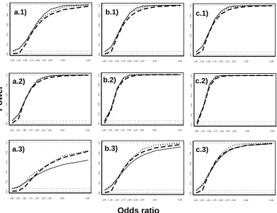
Figure 1 compares the power of the non-signed tests for excluding edge (1,2) from the saturated GLL model with two binary variables, using the normal approximation (dashed line) and the non-central chi-squared approximation (solid line), for different combinations of marginal probabilities and odds ratio values. The dotted line is the estimated exact power, used as the standard for comparison, based on 1 000 simulations. Note that there are only three curves in each panel, rather than nine, because the power functions are essentially the same for each test statistic. A sample size of 1 000 was used. The horizontal dotted lines correspond to power values of 0 and 0.05. In each plot the odds ratio, on the horizontal axis, varies from 1 to 4. The marginal probabilityπ1(0) takes the values 0.1, 0.5 and 0.9 in the plots in rows 1 to 3, respectively. The marginal probability π2(0) takes the values 0.1, 0.2 and 0.3 in the plots in columns a) to c), respectively.

From Figure 1 it is possible to conclude that, even for a sample size of 1 000, the normal approximation is a poor approximation for values of the odds ratio close to one. Indeed, at an alternative close to the null the non-central chi-squared approximation performs much better. When the odds ratio value is far from one and π1(0) is around 0.9, the normal approximation performs better than the non-central chi-squared approximation (see the plots in row 3). Note that, in such cases, the minimum expected cell counts can be very small: in plot a.3) values of 3.8 and 2.9 are reached for ψ12 equal to 3 and 4, respectively. The chi-square approximation is very poor then. The non-central chi-squared approximation performs very well when π1(0) is around 0.5 (see the plots in row 2).

For a sample size of 10 000 (considered a very large sample size for a GLL model with two binary variables) the normal approximation is still a poor approximation for odds ratio values close to one. Also the non-central chi-squared approximation performs better than the normal approximation. For further details see Salgueiro [5].

1,001,251,501,752,002,252,50 3,00 4,00 0.0 0.2 0.4 0.6 0.8 1.0 a.1)

1,001,251,501,752,002,252,50 3,00 4,00

0.0 0.2 0.4 0.6 0.8 1.0 a.2) Power

1,001,251,501,752,002,252,50 3,00 4,00

0.0 0.2 0.4 0.6 0.8 1.0 a.3)

1,001,251,501,752,002,252,50 3,00 4,00

0.0 0.2 0.4 0.6 0.8 1.0 b.1)

1,001,251,501,752,002,252,50 3,00 4,00

0.0 0.2 0.4 0.6 0.8 1.0 b.2)

1,001,251,501,752,002,252,50 3,00 4,00

0.0 0.2 0.4 0.6 0.8 1.0 b.3) Odds ratio

1,001,251,501,752,002,252,50 3,00 4,00

0.0 0.2 0.4 0.6 0.8 1.0 c.1)

1,001,251,501,752,002,252,50 3,00 4,00

0.0 0.2 0.4 0.6 0.8 1.0 c.2)

1,001,251,501,752,002,252,50 3,00 4,00

0.0 0.2 0.4 0.6 0.8 1.0 c.3)

Fig. 1. Simulated (dotted line) and theoretical power values forT₁₂,with an asymp-totic normal approximation (dashed line) and a non-centralχ2₁ approximation (solid line);n_∅= 1 000. Odds ratioψ12from 1 to 4 in each plot.π1(0) equals: 1) 0.1, 2) 0.5 and 3) 0.9. π₂(0) equals: a) 0.1, b) 0.2 and c) 0.3. The horizontal dotted lines cor-respond to power values of 0, 0.05 and 1.

i.e., of selecting the true (saturated) model has been termed overall power in the multiple comparisons literature (see, for example, Hochberg and Tamhane [9]).

In the three binary variables case the probability of excluding neither of the two edges (i, j) and (i, k) from the saturated GLL model, when two separate edge exclusion tests are performed, can be approximated by

P hmin(Tij, Tik)> χ22;1−α|ξ

i '

Z ∞

χ2

2;1−α

Z ∞

χ2

2;1−α

φ2(µ, Σ) dTij dTik, (11)

The power of selecting the saturated GLL model with three binary variables is the probability that each of the test statisticsT12, T13 and T23 is greater than

χ2

2;1−α, given the values of the chosen parameters in ξ. A generalization of

Equation (11), with a three-dimensional integral, can be used to approximate this power.

4.2 Power of signed square-root tests

Recall that, in the two binary variables case, signed square-root test statistics

Ts

12 equal sign(log ˆψ12) √

T12, whereT12 is one of the non-signed test statistics given by Equations (1) to (3).

For a two-sided test of size α, the null hypothesis that λ12 = 0 ⇔ ψ12 = 1 is rejected if the absolute value of the signed square-root test statistic is greater thanz1−α/2, wherez1−αis the upperαquantile of the standard normal

distribution. Hence, the power for the two-sided size α signed square-root test of excluding edge (1,2) from the saturated GLL model with two binary variables can be approximated by

P£

|T₁₂s_|> z_1−α/2|ξ¤

'P

"

Z < zα/2−AE(T

s

12)

p

var(T₁₂s)

#

+P

"

Z > z1−α/2−AE(T

s

12)

p

var(T₁₂s)

#

,

(12) where Ts _{is the signed square-root version of the test statistic of interest,}

with mean and variance, in the asymptotic distribution, given by AE(Ts

12) and var(Ts

12). The power for a one-sided test of size α/2 is approximated by either the first or the second term on the right-hand side of Equation (12), depending on the direction of the alternative hypothesis.

Simulation results (Salgueiro [5]) showed that the normal approximation to the power of the signed square-root tests of excluding edge (1,2) from the sat-urated model is a very good approximation, even for moderate sample sizes, marginal probabilities close to zero or one and odds ratio values close to one. Her simulation results also showed that the asymptotic normal approximations are more accurate for the signed square-root versions than for the non-signed versions, suggesting that, when there is a choice, signed square-root test statis-tics should be preferred.

5 An Example: University Admissions

orf) and department (D: 3 or 4) are investigated. For these data, ˆψGA = 1.02

and, conditioning on D, ˆψGA·D=3 = 1.13 and ˆψGA·D=4 = 0.92. For n∅ = 1710, the LRT statistic for H0 : G⊥⊥A|D is 1.05, with a p-value of 0.59, and a backward elimination model selection procedure chooses model GD, A (α = 0.05). Hence, there is no evidence of gender discrimination in the admission process for departments 3 and 4.

To investigate the power associated with this LRT and this model selection procedure, values of ˆψGA·D=3 and ˆψGA·D=4 more extreme than the observed are considered. The five remaining parameters in ξ are selected to be the marginal probability ofD= 3,πD(3), the probabilities ofG=mgivenD=d,

πG·D(m, d),and the probabilities of A=ygiven D=d, πA·D(y, d). These five

parameters are set close to their observed values: πD(3) = 0.54, πG·D(m,3) =

0.35, πG·D(m,4) = 0.53 andπA·D(y,3) =πA·D(y,4) = 0.35.

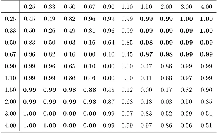
For the LRT of H0 : G⊥⊥A|D, the power is greater than 0.62 (0.88) if one (both) of ˆψGA·D=3 and ˆψGA·D=4 is (are) outside (0.67,1.50). Hence, a sample of 1710 has enough power to detect a substantively interesting (conditional) association between Gand A. For the power of selecting the saturated model the picture is less clear, as can be seen from Table 1. If one of the conditional odds ratios is less than 0.67 and the other is greater than 1.50 then the power is greater than 0.87. However, if they are both less than 0.67 or both greater than 1.50 then the power can be much lower. This is because for such values of ˆψGA·D

and the remaining values of ξ set close to their observed values, the induced conditional association betweenAandDis small and hence the corresponding edge is not required in the model. The results in Table 1 highlight the need for care when specifying the values inξto ensure that power calculations relevant to the hypotheses of interest are being performed.

6 Discussion

Table 1

Power of selecting the saturated model for various values of ˆψGA·D=3 (in rows) and ˆ

ψ_GA·D=4 (in columns);n∅= 1710.

0.25 0.33 0.50 0.67 0.90 1.10 1.50 2.00 3.00 4.00

0.25 0.45 0.49 0.82 0.96 0.99 0.99 0.99 0.99 1.00 1.00

0.33 0.50 0.26 0.49 0.81 0.96 0.99 0.99 0.99 0.99 1.00

0.50 0.83 0.50 0.03 0.16 0.64 0.85 0.98 0.99 0.99 0.99

0.67 0.96 0.82 0.16 0.00 0.10 0.45 0.87 0.98 0.99 0.99

0.90 0.99 0.96 0.65 0.10 0.00 0.00 0.47 0.86 0.99 0.99

1.10 0.99 0.99 0.86 0.46 0.00 0.00 0.11 0.66 0.97 0.99

1.50 0.99 0.99 0.98 0.88 _{0.48 0.12 0.00 0.17 0.82 0.96}

2.00 0.99 0.99 0.99 0.98 _{0.87 0.68 0.18 0.03 0.50 0.85}

3.00 1.00 0.99 0.99 0.99 _{0.99 0.97 0.83 0.52 0.29 0.54}

4.00 1.00 1.00 0.99 0.99 _{0.99 0.99 0.97 0.86 0.56 0.51}

References

[1] A. Agresti, Categorical Data Analysis, John Wiley & Sons, New Jersey, 2nd edition, 2002.

[2] D. Edwards, Introduction to Graphical Modelling, Springer-Verlag, New York, 2nd edition, 2000.

[3] S.L. Lauritzen, Graphical Models, Clarendon Press, Oxford, 1996.

[4] J. Whittaker, Graphical Models in Applied Multivariate Statistics, John Wiley & Sons, Chichester, 1990.

[5] M.F. Salgueiro, Distributions of Test Statistics for Edge Exclusion for

Graphical Models, Ph.D. Thesis, University of Southampton, 2003.

[6] P.W.F. Smith, Edge Exclusion and Model Selection in Graphical Models, Ph.D. Thesis, Lancaster University, 1990.

[7] D. Cox, D. Hinkley, Theoretical Statistics, Chapman & Hall, 1974.

[8] Y. Bishop, S. Fienberg, P. Holland,Discrete Multivariate Analysis: Theory

and Practice, MIT Press, Cambridge, Massachusetts, 1975.

[9] Y. Hochberg, A. Tamhane, Multiple Comparison Procedures, John Wiley & Sons, Chichester, 1987.