Control-focused, nonlinear and time-varying modelling of dielectric elastomer actuators with frequency response analysis

dielectric elastomer actuators with frequency response analysis. White Rose Research Online URL for this paper:

http://eprints.whiterose.ac.uk/90689/ Version: Accepted Version

Article:

Jacobs, W.R., Wilson, E.D., Assaf, T. et al. (4 more authors) (2015) Control-focused, nonlinear and time-varying modelling of dielectric elastomer actuators with frequency response analysis. Smart Materials and Structures, 24 (5). ISSN 0964-1726

https://doi.org/10.1088/0964-1726/24/5/055002

eprints@whiterose.ac.uk https://eprints.whiterose.ac.uk/ Reuse

Unless indicated otherwise, fulltext items are protected by copyright with all rights reserved. The copyright exception in section 29 of the Copyright, Designs and Patents Act 1988 allows the making of a single copy solely for the purpose of non-commercial research or private study within the limits of fair dealing. The publisher or other rights-holder may allow further reproduction and re-use of this version - refer to the White Rose Research Online record for this item. Where records identify the publisher as the copyright holder, users can verify any specific terms of use on the publisher’s website.

Takedown

If you consider content in White Rose Research Online to be in breach of UK law, please notify us by

modelling of dielectric elastomer actuators with

frequency response analysis

William R Jacobs1, Emma D Wilson2, Tareq Assaf3, Jonathan

Rossiter3_{, Tony J Dodd}1_{, John Porrill}2 _{and Sean R Anderson}1

1

Dept of Automatic Control and Systems Engineering and Sheffield Centre for Robotics, University of Sheffield, Sheffield, UK

2

Dept of Psychology and Sheffield Centre for Robotics, University of Sheffield, Sheffield, UK

3

Bristol Robotics Laboratory, University of Bristol, Bristol, UK

E-mail: w.jacobs@sheffield.ac.uk,s.anderson@sheffield.ac.uk

September 2014

Abstract. Current models of dielectric elastomer actuators (DEAs) are mostly

constrained to first principal descriptions that are not well suited to the application of control design due to their computational complexity. In this work we describe an integrated framework for the identification of control focused, data driven and time-varying DEA models that allow advanced analysis of nonlinear system dynamics

in the frequency-domain. Experimentally generated input-output data

(voltage-displacement) was used to identify control-focused, nonlinear and time-varying dynamic models of a set of film-type DEAs. The model description used was the nonlinear autoregressive with exogenous input (NARX) structure. Frequency response analysis of the DEA dynamics was performed using generalised frequency response functions (GFRFs), providing insight and a comparison into the time-varying dynamics across a set of DEA actuators. The results demonstrated that models identified within the presented framework provide a compact and accurate description of the system dynamics. The frequency response analysis revealed variation in the time-varying

dynamic behaviour of DEAs fabricated to the same specifications. These results

suggest that the modelling and analysis framework presented here is a potentially useful tool for future work in guiding DEA actuator design and fabrication for application domains such as soft robotics.

PACS numbers: 05.45.-a, 05.45.Tp, 45.80.+r

1. Introduction

Electro-Active Polymers (EAPs) are a rapidly developing class of ‘smart’ material that produce actuation through deformation in response to an applied electric field [1]. EAPs combine a set of promising, desirable properties for actuation including large actuation strains, low mass, high response speed and compliance [2]. Dielectric elastomer actuators (DEAs) are a class of EAP, akin to a compliant capacitor, which show great potential in the replacement of conventional hard actuators for many applications, including robotics [3–5], orthotics and prosthetics [6, 7], and healthcare [8]. The nonlinearity and time-variation in DEA dynamics necessitates the need for advanced control algorithms before their potential in applications can be fully realised [5, 9, 10]. A crucial step therefore, is the development of techniques for control-focused modelling and analysis, which is the subject of this paper.

Early dynamic modelling methods for DEAs made use of linear-elasticity and free boundary approximations to provide a reasonable prediction of DEA behaviour for small strains (<10%) [11, 12]. In order to address the limitations of small strains and linear-elasticity, nonlinear models were considered based on hyperelasticity models [13–15], specialised to describe DEA behaviour [16–18]. A more advanced model of the DEA

response was derived from the viewpoint of thermodynamics in [19]. This latter

contribution provides a model capable of accurately predicting large deformations. Therefore, a range of useful first principal models have been developed for dynamic linear/nonlinear analysis of DEAs.

These first principal models have been useful in driving forward the development of DEAs. However, they are generally not well suited to control-focused analysis and design because they tend to be overly complex descriptions, incorporating many terms and parameters. Furthermore, DEAs tend to exhibit time-varying characteristics which most current models do not describe, or are limited to a simplified assumption of time varying phenomena [18,20]. There is, therefore, a significant gap in the current methodology for modelling DEAs in control-oriented tasks. Hence, it is now timely to develop modelling approaches for DEAs that are specifically control-focused due to the increased use of DEAs in various applications, including for example, soft robotics [4, 5, 21].

The aim of this paper is to develop a novel framework for control-oriented modelling and analysis of DEAs using data-driven system identification methods. The developed framework is based on the nonlinear autoregressive with exogenous input (NARX) model [22, 23]. The NARX model provides a number of advantages related to control: it tends to produce simple, compact, and accurate models, naturally incorporating a description of plant nonlinearities [24]. In addition, it is a linear-in-the-parameters model suited to the time-varying estimation of DEA dynamics.

NARX models are widely used to describe dynamic systems, e.g. in power

and Bayesian inference [30]. A simulation prediction error identification approach is taken here, which tends to improve model term selection for fast-sampled data [23, 31]. A key attribute of the framework developed in this investigation is the use of generalised frequency response functions (GFRFs) [32] - for the first time allowing

frequency response analysis of nonlinear and time-varying DEA dynamics. The

advantage of using GFRFs stems from the fact that the identified NARX model equations are difficult to interpret and directly use for analysis. However, the frequency response is a powerful, widely used method in control for interpreting system dynamics [23]. The GFRF methodology extends the use of frequency response analysis from linear models (i.e. the Bode plot) to nonlinear models.

Furthermore, the time-variation of model parameters is also difficult to interpret directly but here we extend the GFRF analysis to the time-varying case, similarly to the approach taken in [33]. This provides much clearer insight into the time-varying dynamics of the DEAs than examining the time-variation of the model parameters alone. The resulting modelling-analysis framework is demonstrated on six film-type DEAs in an experimental setup, providing insight into the dynamic similarities and differences across this set of actuators.

In section 2 the methods used in this work are detailed, which includes a description of the experimental set-up used for generating input-output data, the nonlinear system identification algorithm and the frequency response analysis methods. In section 3 the results of system identification and frequency response analysis of the DEAs are presented. A discussion of the investigation is made in section 4 and the main conclusions are drawn in section 5.

2. Methods

System identification is the process of building mathematical models of dynamic systems from measured data. A key difference of system identification from other modelling approaches is that one does not have to assume knowledge of the dynamics in a specific form, e.g. a nonlinear differential equation with known terms. Instead, the dynamic model can be obtained entirely from data (model structure as well as parameters). In general, the linear system identification process follows a distinct logical progression, from collection of the input-output data, to model identification, then model validation. This process is often refined for nonlinear system identification to account for the problem of term selection, where many possible terms must be searched to form the nonlinear model.

In this section, we describe the system identification framework used to model and analyse a set of DEAs. Firstly, we outline the DEA experimental setup and the data collection process, where the input is the voltage that activates the DEA and the measured output is displacement of the DEA. We then give details of the nonlinear system identification approach assuming time-invariance of the DEA, which

A

Laser displacement sensor

DEAP

X

Laser displacement sensor (output) DEAP

y

Voltage input signal B

C

0 500 1000 1500

2 4

Input

Time [s]

Voltage [V]

0 500 1000 1500

0 2

3 Output

Time [s]

Displacement [mm]

1

E

Voltage [V]

1 1.5 2 2.5 3 3.5

Displacement [mm]

0 1 2 3

0 500 1000 1500

Time [s]

0.2 0.4 0.6 2 3

Voltage [V]

Displacement [mm]

Time [s]

Time [s]

0 10 20 30 40 50 60

0 10 20 30 40 50 60

D

F

Figure 1. Experimental set-up. (A) Photograph of the dielectric elasotmer atuator, a

spherical metal mass plasced on a film of DE material stretched over a perspex frame. (B) The vertical displacement (system output) of a spherical mass is measured by a laser displacement sensor (system input). (C) Top: Input signal,u, for DEA1. Bottom:

Output signal, y, for DEA1.(D)Input signal, u, for DEA1 (E) Input vs. output for

DEA1, time is indicated by the colour scale. (F) Output signal,y, for DEA1.

recursive approach to parameter estimation for a given NARX structure, to model the time-varying DEA dynamics. Finally, the analysis method of the NARX model using frequency response functions is described.

2.1. Experimental setup

The experimental data used in this investigation was obtained by independently driving a set of six DEAs, with voltage as the input and displacement measured as the output. The experiment was designed so that the displacement of the actuator could be measured in a simple one-dimensional movement direction [5] (Fig. 1A-B). The input output data were chosen as pre-amplified voltage and displacement respectively in order that they correspond to the properties that the user wants to directly control.

compliant electrodes. During activation the electrodes were squeezed together in response to an applied voltage, causing biaxial expansion of the elastomer film, inducing actuation.

The experimental set up comprised of a circular acrylic elastomer (3M VHB 4905) fixed to a rigid perspex frame with inner and outer diameters of 80mm and 120mm respectively. The elastomer was biaxially prestrained by 350%. Conductive carbon grease (MG chemicals) was smeared on both sides of the elastomer to form circular electrodes, the electrodes were approximately circular, diameter ≈ 35mm. A spherical 3g mass was placed at the centre of the circular DEA allowing a vertical displacement to be measured with a laser displacement sensor (Keyence LK-G152), in response to an applied voltage (Fig. 1A-B).

A host Laptop combined with a CompactRio (CRIO-9014, National Instruments) platform, with input module 9144 (National Instruments) and output module NI-9264 (National Instruments) was used for the data acquisition.

Input (voltage) and output signals (displacement) were sampled at 50Hz. Voltages in the range 1.1V-3.75V were produced by the CRio output module and amplified with the ratio 15V:12kV before being fed into the DEA. The excitation signal was formed of band limited Gaussian white noise (0-1Hz). The signal measured by the laser displacement sensor in response to the applied voltage was supplied to the input module of the CRio.

2.2. Identification of the nonlinear model structure

In a preliminary analysis of input-output data the displacement signal of the DEA was shown to be non-stationary, indicating time-varying dynamic behaviour (Fig. 1C). In addition, from an initial analysis of the data, the form of the nonlinearity appeared to remain the same over time . This conclusion was reached by observing that the shape, or functional form, of the voltage displacement relationship was a approximately quadratic nonlinearity that only varies in average displacement over time (Fig. 1E). Therefore we assumed that the DEA could be described by a fixed nonlinear model structure with time-varying parameters (later validated as part of the model identification procedure - see Results). This section describes the identification of the fixed nonlinear model structure, whilst the subsequent section extends the identification to the time-varying case assuming a known model structure. The methods described here were applied to a short (100 second) segment of data, where the dynamics were assumed to be well approximated by a time-invariant model.

The nonlinear system identification procedure assumes that we can describe a single-input single-output dynamic system as some nonlinear function, f(.) of lagged system inputs, ut and outputs, yt,

yt=f(xt) +et (1)

where xt = yt−1, ..., y_t−_ny, u_t−1, ..., u_t−_nu

and et is a normally distributed white noise

respectively. We decompose the nonlinear function f(.) into a sum of weighted basis functions, which is a linear-in-the-parameters model,

f(xt) = m

X

j=1

θjφj(xt) (2)

whereθj is the jth model parameter andφj(xt) is in this case a polynomial basis function

transformation of lagged input-output signals. The NARX model parameters can be estimated for a time-invariant model structure in closed form using the least-squared error criterion,

JLS(θ) =

1 N N X t=1 1

2(yt−φtθ) 2

(3)

whereφ_t= (φ1(xt), ..., φm(xt)),θ = (θ1, . . . , θm)T and m is the number of model terms.

The least-squares parameter estimates are then given by

ˆ θLS =

1

N

N

X

t=1 φT_tφ_t

!−1

1

N

N

X

t=1

φT_tyt (4)

The model structure was identified here using a simulation based term selection algorithm [31], which has been shown to provide greater discrimination between model terms than one-step-ahead predictive algorithms [31]. Term selection for the NARX model was done by an iterative algorithm, driven by the simulated error reduction ratio (SERR), where

SERRi =

M SSE(Mi)−M SSE(Mi+1)

1 N N P t=1 y2 t (5)

where Mi is the model at the ith iteration andMi+1 is the model to be tested at the

subsequent iteration. M SSE is the Mean Squared Simulation Error, given by

M SSE= 1

N

N

X

i=1 ˆ

e2i (6)

where ˆei =yi−yˆi, with ˆyi being the simulated system output at timet =i given by

ˆ

yt= m

X

j=1 ˆ

θjφj(ˆxt) (7)

where

ˆ

xt = ˆyt−1, ...,yˆt−n_y, ut−1, ..., ut−n_u

(8)

is a vector of lagged simulated system input terms and system output terms at timet. The structure detection algorithm proceeds as follows: some initial model structure, M0, is chosen. Typically this is composed of a linear basis of a predefined dynamic order.

SERR0 is initialised as

SERR0 =

M SSE(M0) 1

N

P

tyt2

At theith iterationSERRi is calculated by equation (5) for a proposed modelMi. The

proposed modelMi consists of the model chosen at the previous iteration,Mi−1, plus a

basis function from the set of all remaining basis functions, where each unselected basis

function is tested one at a time. The model Mi that produces the minimum value of

SERRi is then chosen and the newly selected basis function is removed from the set

of remaining basis functions. The algorithm ends when SERRi−SERRi−1 falls below

a predefined threshold, indicating that no significant increase in model quality can be gained by the addition of a further basis function.

Redundant terms are pruned from the model using a pruning algorithm following the same procedure as the structure detection algorithm but removing a term at each iteration until a threshold is reached. Model parameters are necessarily re-estimated for each proposed model by equation (4).

2.3. Estimation of time-varying parameters

The time-invariant model described above was extended to account for time-varying dynamics by allowing the parameters to vary as a function of time,

f(xt,θt) = m

X

j=1

θj(t)φj(xt) (10)

where θt = (θ1(t), . . . , θm(t))T. Time-varying model parameters were estimated using a

recursive least squares (RLS) algorithm with a regularisation term included to prevent any terms from dominating due to noise effects [34]. The RLS algorithm minimises this cost function at time-step n,

JRLS(θ, n) = n

X

t=1

kyt−φtθk2+αkθk2

+θ−θˆ0

T

P−1

0

θ−θˆ0

(11)

The first term in equation (11) is the model prediction error. The second term is a standard regularisation term, with α being a constant. The third term is introduced in order to enforce a constant effect at each sample. Here, P0 = δ−1I with δ > 0. The algorithm for minimising JRLS(θ) is [34],

K∗

n=αPn−1(I+αPn−1) −1

(12)

P∗

n =Pn−1−K ∗

nPn−1 (13)

Kn=P

∗

nφn(I+φ T nP

∗

nφn)

−1

(14) θn = ˆθn−1−K

∗

nθˆn−1 +Knφ

T

nK

∗

nθˆn−1+Kn(yn−φ_nθn−1) (15)

Pn =P

∗

n−KnφTnP

∗

n (16)

This formulation of the RLS problem leads to a solution that efficiently and accurately tracks changing model parameters in response to changes in the system dynamics.

2.4. Frequency-domain analysis

are simple methods for obtaining the frequency response function (FRF),H(jω), from a linear system identified in the time-domain (e.g. using Laplace or Z-transforms) [35]. For nonlinear systems, the process of obtaining the frequency response is more complicated than for linear systems but is similarly attractive for the purpose of analysis. The frequency response for nonlinear systems is described by multiple FRFs, known as the generalised frequency response functions (GFRFs) [23]. These GFRFs can be obtained analytically from identified NARX models. The process is described below.

First consider that NARX models of nonlinear systems, such as that given by (1), can also be described by the Volterra series model for which the GFRF is defined. The discrete Volterra series is given by [36]

yt=

∞ X

n=1

yt(n) (17)

where

yt(n) =y(0) + t

X

n=0

. . .

t

X

n=0

hn(k1, . . . , kn) n

Y

i=1

u(t−ki) (18)

is the n’th order output of the system and hn(k1, . . . , kn) is the n-th order impulse

response of the system. Note the inclusion of the 0th order term y(0). This term

is often assumed to be zero in order to simplify the analysis, however, for a system that has non-zero steady state for zero input this assumption is not justified and must be included [37]. The n-th order GFRF, Hn(jω1, . . . , jωn), is found from the

multi-dimensional Fourier transform of the n-th order impulse response.

Hn(jω1, . . . , jωn) =

∞ X

ω1=−∞

. . .

∞ X

ωn=−∞

hn(k1, . . . , kn)e

−j(ω1k1+...+ωnkn) ₍₁₉₎

The estimation of Volterra series models and their transformation is, however, a computationally intensive task due to the huge size of the required parameter space. The probing (or exponential input) method provides a technique for equating Volterra

models with models of some other form, M. This allows the nth order FRF, Hn, to

be described in terms of the parameters of M and hence making the problem more

tractable. For models, M, of the NARX class efficient methodologies and algorithms

can be found in the literature [32, 38, 39].

In the probing method, the Volterra series model is excited by an input formed of a combination of exponentials

ut= M

X

i=1

ejωit ₍₂₀₎

The procedure of obtaining the GFRF from a NARX model by the probing method is best understood by an example. Consider an identified NARX model given by‡,

yt=θ1+θ2yt−1+θ3yt−2+θ4ut−1+θ5ut−2+θ6ut−3+θ7yt−1u

2

t−1

+θ8yt−1ut−2ut−3+θ9yt−1u

2

t−3+θ10yt−2u

2

t−1 (21)

Applying an input of the form

ut=e(jω1t)+e(jω2t) (22)

the delayed lag terms are

ut−1 =e

(jω1(t−1))

+e(jω2(t−1))

(23)

and the output response is given by [32]

y(k) =y0+H1(jω1)ejω1t+H2(jω2)ejω2t+ 2!H2(jω1, jω2)ej(ω1+ω2)t

+H2(jω1, jω1)e2jω1t+H2(jω2, jω2)e2jω2t (24)

where all terms higher than second order have been omitted. Lagged output terms follow directly from equation (24). The first order FRF can then be obtained by Substituting (23) and (24) and their lagged forms into the time-domain NARX model given by equation (21) and comparing coefficients of either ejω1t

or ejω2t

leads to the following equation

H1(jω1) =θ2H1ejω1(k

−1)

+θ3H1ejω1(k

−2)

+θ4ejω1(k

−1)

+θ5ejω1(k

−2)

+θ6ejω1(k−3)+y0θ9 (25)

where the zero input response y0 can be found from solving the following equation

y0 =θ1+θ2y0+θ3y0 (26)

The first order FRF of the system is hence given by

H1(jω1) = θ4e

−_jω5 +θ

5e−2jω1 + (θ6+y0θ9)e−3jω1 1−θ2e−jω1 −θ3e−2ω1

(27)

The second order FRFs can be obtained by equating the coefficients ofej(ω1+ω2) to give

H2(jω1, jω2) =θ2H2(jω1, jω2)e

−_j(_ω1+ω2)

+θ3H2(jω1, jω2)e

−2_j(_ω1+ω2)

+1 2y0θ7e

−2j(ω1+ω2)

+ 1

2y0θ8(e

−j(2ω1+3ω2)

+e−j(3ω1+2ω2)

)

+1

2y0θ9(H1(jω1)e

−j(ω1+3ω2)

+H1(jω2)e−j(3ω1+ω2)

)

+1 2y0θ10e

−2j(ω1+ω2)

(28)

hence

H2(jω1, jω2) =

A(jω1, jω2)

B(jω1, jω2)

(29)

‡ Note that this NARX model is in fact the identified structure of DEA1 as reported in the results

where

A(jω1, jω2) =

y0

2(θ7+θ10)e

−2j(ω1+ω2)

+ y0 2θ8(e

−j(3ω1+2ω2)

+e−j(2ω1+3ω2)

)

+1

2θ9(H1(jω1)e

−j(ω1+3ω2)

+H1(jω2)e−j(3ω1+ω2) (30)

and

B(jω1, jω2) = 1−θ2e

−j(ω1+ω2)

−θ3e

−2j(ω1+ω2)

(31)

Therefore, by the using the identified NARX model and the probing method it is possible to obtain analytic expressions defining the frequency response of the nonlinear system. The method can readily be extended to the time variant case by the introduction of time dependant parameters such that the FRFs become a function of time, H(jω, t). Time dependant FRFs provide a useful analytic tool for the visual analysis of DEAs. Time-frequency plots can be generated by plotting the magnitude,|H(jω, t)|, and phase, ∠H(jω, t), of the first order FRFs.

2.5. Identification and analysis procedure

The displacement response of six circular DE film actuators were measured in response to a band limited Gaussian input voltage according to the procedure described in section 2.1. The use of band limited white noise as an excitation signal is standard in nonlinear system identification as it is persistently exciting and leads to identifiability of the system [40, 41] whilst providing a simple design for the input signal (just the choice of frequency band). Other choices of input signals (such as periodic multisines) are also valid so long as they are persistently exciting across the bandwidth of the system [23]. The experiment was designed in order to capture the dynamic behaviour of the system as well as its time varying characteristics.

In order to identify the nonlinear model structure, the dynamic orders (ny, nu) and

polynomial order (np) for the model were first estimated. Various methods exist for

the selection of suitable variables relating to the polynomial and dynamic order. A standard method is based on the identification of linear models of the system [42] and the approach used here is based on this method. The required dynamic orders can therefore be inferred by comparison of linear models, i.e. a NARX model of polynomial order np = 1. As such, linear models were identified using the method in section 2.2

with increasing dynamic order, ny =nu = 1, . . . ,5. With the dynamic and polynomial

orders fixed, the nonlinear structure was identified using the the method in section 2.2. A comparison of the goodness of fit for each model was made using independent validation data, considering both the normalised mean square error (NMSE) and final prediction error (FPE), where

N M SE= 1−

PN

t=1(yt−yˆt)2

PN

t=1(yt−y¯)2

where ¯y= 1/NPN

t=1yt, and

F P E= 1/N

N

X

t=1

(yt−yˆt)2

1 +d/N

1−d/N

(33)

where d is the number of model terms.

The RLS method for time-varying parameter estimation, described in section 2.3, was used to track the parameters of the system over the entire 30 minute data set. To analyse the time-varying frequency response, GFRFs for the identified time-varying models were then calculated following the procedure described in section 2.4.

3. Results

3.1. Identification of NARX model structure

The DEAs display a linear dynamic response from approximately 1.5V to 3V. When the voltage exceeds approximately 3V the actuators enter a nonlinear mode, (Fig. 1E). It is clear from the raw data that the actuators also exhibit hysteresis as well as time-varying characteristics (Fig. 1C,E).

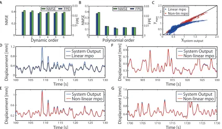
When identifying the linear model, to fix the dynamic order, the model fit was increased gradually from first to third order dynamics (Fig. 2A). After third order dynamics the model fit for both measures flattens off. This behaviour is expected when no more information can be obtained by the addition of higher order regressors and the rise in model complexity is relatively small. This is then used to justify the exemption of terms higher than order three from the model identification step.

From observation of the experimental input-output data it is clear that it is necessary to consider the nonlinearities of the system in order to accurately capture the dynamics (Fig. 1C,E). In order to select an appropriate polynomial order to model the nonlinearities another comparison across polynomial orders with dynamics set to second order was carried out. The best choice of dynamic order was found to be third (Fig. 2B).

NARX models identified using the simulation-based algorithm, described in section 2, accurately captured the dynamics of the system, demonstrated by simulation comparison with an independent validation data set (Fig. 2C,E-G). Linear models displayed consistent errors, where the full amplitude of the DEA response was not captured (Fig. 2D). Nonlinear models in contrast described the full range of dynamic, justifying the use of nonlinear modelling (Fig. 2C,E-G).

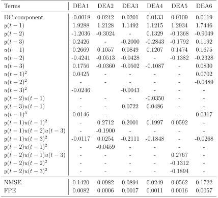
The identified NARX models show some consistency in term selection, notably in the choice of y(t−1)u(t−3)2 _{and y(t−1)u(t−2)}2 _{as well as in the linear terms (table} 1). The relatively poor fit of DEAs 1 and 6 can be explained by the presence of rapid time varying dynamics within the test data of these samples.

0 0.2 0.4

1 2 3 4 5 6 0 0.01 0.02 0.03

0 0.5 1 1.5 2 2.5 0 0.5 1 1.5 2 2.5 ympo

ysystem output

100 105 110 115 120 125 130 0 0.4 0.8 1.2 Displacement [mm] Time [s] FPE C D NMSE A 0 0.1 0.2 0.3 0.4 0.5

0 1 2 3 4 5 00 0.01 0.02 0.03 NMSE FPE B 0.2 0.6 1

1700 1705 1710 1715 1720 1725 1730 0.4 0.8 1.2 1.6 System Output Linear mpo

900 905 910 915 920 925 930 0.1 0.3 0.5 0.7 0.9 1 Displacement [mm] Time [s]

100 105 110 115 120 125 130 _{Displacement [mm]}

Time [s] Time [s] Displacement [mm] F G System Output Non-linear mpo E System Output Non-linear mpo System Output Non-linear mpo Linear mpo Non-lin mpo

NMSE FPE NMSE FPE

Dynamic order Polynomial order

Figure 2. (A) Comparison of the goodness of fit for linear models with increasing

dynamic order for DEA 1. (B) Comparison of the goodness of fit for NARX models with increasing polynomial order for DEA 1. (C) System output vs. model predicted output for a Linear model (blue dots) and the NARX model given by equation (21) (red dots) (D) Linear model predicted output vs system output for DEA 1. System output (blue line), ARX model of dynamic order three (black line). (E-G) Nonlinear model predicted output vs system output for DEA 1 at three separate time periods. The same NARX model structure was used in each case with parameters re-estimated using least-squares, system output (blue line), NARX model given by equation (21) (red line)

time periods (100-130s, 900-930s and 1700-1730s), with parameters re-estimated in each case using least-squares. The model gave accurate predictions in each case (Fig. 2E-G), justifying the assumption that the DEAs could be well modelled using a fixed model structure with time-varying parameters.

3.2. Characterisation of time-varying dynamics

It is clear from the observed data that the actuators are influenced by some form of time-varying dynamics, this can clearly be seen in the changes in DC level and gain for all the DEAs (Fig. 1). The physical interpretation of these dynamics are unknown, however, and it is necessary for the phenomena to be described for the development of a conventional control strategy. The advantage of the NARX model approach is that the underlying phenomena causing time-variation does not need to be known. Instead, the time-variation can be described in the model using the observed data.

Terms DEA1 DEA2 DEA3 DEA4 DEA5 DEA6

DC component -0.0018 0.0242 0.0201 0.0133 0.0109 0.0119

y(t−1) 1.9288 1.2128 1.1492 1.1215 1.2934 1.7446

y(t−2) -1.2036 -0.3024 - 0.1329 -0.1368 -0.9049

y(t−3) 0.2426 - -0.2000 -0.2843 -0.1792 0.1192

u(t−1) 0.2669 0.1057 0.0849 0.1207 0.1474 0.1675

u(t−2) -0.4241 -0.0513 -0.0428 - -0.1382 -0.2328

u(t−3) 0.1756 -0.0360 -0.0502 -0.1087 - 0.0830

u(t−1)2 _{0.0425 - - - - 0.0702}

u(t−2)2 _{- - - - - -0.0489}

u(t−3)2 _{-0.0246 -0.0043 - -}

-y(t−2)u(t−1) - - - -0.0350 -

-y(t−3)u(t−1) - - 0.0722 0.0486 -

-u(t−1)3 _{0.0146 - - - - 0.0317}

y(t−1)u(t−1)2 _{- 0.2712 0.2001 0.1997 0.0592}

-y(t−1)u(t−2)u(t−3) - -0.1900 - - -

-y(t−1)u(t−3)2 _{-0.0117 0.0254 -0.2111 -0.1848 - -0.0268}

y(t−2)u(t−1)2 _{- -0.0459 - - -}

-y(t−2)u(t−1)u(t−3) - - - - 0.2767

-y(t−2)u(t−2)2 _{- - - - -0.1312}

-y(t−2)u(t−3)2 _{- - - - -0.1894}

-NMSE 0.1420 0.0982 0.0894 0.0249 0.0562 0.1722

FPE 0.0082 0.0006 0.0017 0.0011 0.0016 0.0057

Table 1. Identified NARX models for DEA 1-6 and their corresponding parameter

values for each term.

the system dynamics are consistent across the different actuators. Similarly, inspection of identified NARX models of the different DEAs shown in table 1 does not reveal whether the DEAs have consistent/inconsistent dynamics. However, the frequency response of the system plotted as a function of time provides a common description that allows direct comparison (Fig. 3).

Some features of the frequency response plots are broadly consistent. All the DEAs exhibit the behaviour of a low pass filter with varying gains. The time-varying characteristics of the actuators are much more inconsistent. In the case of actuators 2 and 6, the average displacements decrease and increase with time respectively, however, the frequency responses show roughly similar patterns (Fig. 3).

Frequency (Hz) −10 −9 −8 0.8 2 0.4 1.2 1.6

Gain (dB) 0.8

2 0.4 1.2 1.6 Gain (dB) Frequency (Hz) DEA 4 −11 −10 −9 −8 −7 DEA 3 −11 0 1 2 3 Frequency (Hz) DEA 5 −14 −13 −12 −11 −10 0.8 2 0.4 1.2 1.6 Gain (dB) Frequency (Hz) DEA 6 −12 −10 −8 0.8 2 0.4 1.2 1.6 Gain (dB) 1 2 0 1 2 3 4 0 −14 −16 Gain (dB) Frequency (Hz) DEA 2 −20 −15 −10 0.8 2 0.4 1.2 1.6 −1 0 1 2 3 Disp [mm] Time [s]

200 400 600 800 1000 1200 1400 1600

1 2 3

Disp [mm]

Time [s]

200 400 600 800 1000 1200 1400 1600

Disp [mm]

Time [s]

200 400 600 800 1000 1200 1400 1600

Disp [mm]

Time [s]

200 400 600 800 1000 1200 1400 1600

Disp [mm]

Time [s]

200 400 600 800 1000 1200 1400 1600

Frequency (Hz) DEA 1 −13 −12 −11 Gain (dB) 0.8 2 0.4 1.2 1.6 0 1 2 3 Disp [mm] Time [s]

200 400 600 800 1000 1200 1400 1600

Gain (dB)

Figure 3. Gain of the First order FRF,|H(jω, t)|, against time for DEAs 1-6, together

with their corresponding raw time series data. All the DEAs display inconsistent time varying dynamics. Time-frequency behaviour is not intuitive from time domain behaviour alone.

dyamics.

4. Discussion

The identified NARX models were found to accurately predict dynamics of the DEAs on independent validation data, and greatly improved on the prediction accuracy of identified linear models.

The need to use nonlinear models to accurately describe DEA dynamics, found here, is consistent with current models of DEAs derived by considering the physical properties of the material [20, 43–45]. A distinct, novel contribution of the work presented here is that the NARX models identified are compact difference equation descriptions with few terms, unlike many of the physical models, making them particularly amenable to control design. Further to this, the NARX modelling framework is able to represent a broad range of nonlinear systems because the model class can be used to describe general multiple-input multiple-output (MIMO) systems with a defined input and output [46]. Therefore, it is likely that the modelling and analysis framework could be applied to a wider range of actuator configurations in the future.

Recursive parameter estimation was combined with GFRF analysis to investigate the time variation of the DEA dynamics in the frequency-domain - a more interpretable approach than examining the time-evolution of the model parameters alone. Describing time variations in DEAs has not been addressed by the EAP community to date and are important because they provide difficulties for implementing a control scheme. Time variations due to relaxation have been studied by [20], however they are not able to explain the behaviour discussed in this work.

Currently the literature provides few examples of adaptive control algorithms for DEAs that would successfully handle time-variation, although success has been made by the use of bioinspired techniques [5]. The control-focused modelling framework proposed here and applied to film-type DEA actuators should enable future high precision control designs that can handle nonlinearity and time-variation of this actuator-type. As the modelling and analysis framework is generically applicable to many system-types, it is likely that the framework could be applied in future to different actuator configurations. A potential future use of the methodology is in guiding fabrication of film-type DEAs. For instance, fabrication parameters of the film-type DEA such as polymer diameter could be included in the NARX model [47]. These fabrication parameters could then be optimised to achieve a desired frequency response for a control application using the NARX model and GFRF analysis. Model-based guiding of the manufacture of film-type DEAs would be a novel approach to fabrication, closely integrating desired dynamic performance characteristics with the manufacturing process.

5. Conclusions

In this paper, we have developed a framework for the identification of control-focused models of dielectric elastomer actuators, describing the nonlinear and time-varying

dynamics. We have extended this identification approach with a methodology for

models, a feature not permitted by directly examining the nonlinear model equations. Application of the modelling and analysis framework to a set of six DEAs revealed that actuators fabricated using the same method exhibited quite different dynamics and time-variation. These results have demonstrated that the methodology can be successfully used to analyse the complex nonlinear and time-varying dynamic behaviour of film-type DEAs.

Acknowledgments

The authors gratefully acknowledge that this work was supported by the Engineering and Physical Sciences Research Council (EPSRC) UK grant “Bioinspired Control of Electro-Active Polymers for Next Generation Soft Robots” (EP/I032533/1) and an EPSRC doctoral training grant to W. Jacobs.

References

[1] Y. Bar-Cohen. Electroactive polymer (EAP) actuators as artificial muscles: reality, potential, and challenges. SPIE Press, 2004.

[2] A. OHalloran, F. OMalley, and P. McHugh. A review on dielectric elastomer actuators, technology, applications, and challenges. Journal of Applied Physics, 104(7):071101, 2008.

[3] J. D. Madden. Mobile robots: motor challenges and materials solutions. Science, 318(5853):1094– 1097, 2007.

[4] C. T. Nguyen, H. Phung, T. D. Nguyen, C. Lee, U. Kim, D. Lee, H. Moon, J. Koo, J. Nam, and H. R. Choi. A small biomimetic quadruped robot driven by multistacked dielectric elastomer actuators. Smart Materials and Structures, 23(6):065005, 2014.

[5] E. D. Wilson, T. Assaf, M. J. Pearson, J. M. Rossiter, S. R. Anderson, and J. Porrill. Bioinspired

adaptive control for artificial muscles. In Biomimetic and Biohybrid Systems, volume 8064,

pages 311–322. Springer Berlin Heidelberg, 2013.

[6] F. Carpi, S. Raspopovic, and D. De Rossi. Activation of dielectric elastomer actuators by means of human electrophysiological signals. InProc. SPIE 6168, page 61681B, 2006.

[7] H. M. Herr and R. D. Kornbluh. New horizons for orthotic and prosthetic technology: artificial

muscle for ambulation. InProc. SPIE 5385, pages 1–9, 2004.

[8] S. Pourazadi, S. Ahmadi, and C. Menon. Towards the development of active compression bandages using dielectric elastomer actuators. Smart Materials and Structures, 23(6):065007, June 2014.

[9] M.Y. Ozsecen and C. Mavroidis. Nonlinear force control of dielectric electroactive polymer

actuators. InProc. SPIE 7642, page 76422, 2010.

[10] S. Xie, P. Ramson, D. Graaf, E. Calius, and I. Anderson. An adaptive control system for dielectric

elastomers. InIEEE International Conference on Industrial Technology, pages 335–340, 2005.

[11] R. E. Pelrine, R. D. Kornbluh, and J. P. Joseph. Electrostriction of polymer dielectrics with compliant electrodes as a means of actuation. Sensors and Actuators A: Physical, 64(1):7785, 1998.

[12] I. Krakovsky, T. Romijn, and A. Posthuma de Boer. A few remarks on the electrostriction of elastomers. Journal of Applied Physics, 85(1):628, 1999.

[13] M. Mooney. A theory of large elastic deformation. Journal of Applied Physics, 11(9):582, 1940. [14] R. W. Ogden. Large deformation isotropic elasticity - on the correlation of theory and experiment

[15] O. H. Yeoh. Characterization of elastic properties of carbon-black-filled rubber vulcanizates.

Rubber Chemistry and Technology, 63(5):792–805, November 1990.

[16] M. Wissler and E. Mazza. Modeling of a pre-strained circular actuator made of dielectric

elastomers. Sensors and Actuators A: Physical, 120(1):184–192, April 2005.

[17] N.C. Goulbourne, E.M. Mockensturm, and M.I. Frecker. Electro-elastomers: Large deformation analysis of silicone membranes. International Journal of Solids and Structures, 44(9):2609–2626, May 2007.

[18] J.-S. Plante and S. Dubowsky. On the performance mechanisms of dielectric elastomer actuators.

Sensors and Actuators A: Physical, 137(1):96–109, June 2007.

[19] Z. Suo, X. Zhao, and W. Greene. A nonlinear field theory of deformable dielectrics. Journal of

the Mechanics and Physics of Solids, 56(2):467–486, February 2008.

[20] M. Wissler and E. Mazza. Modeling and simulation of dielectric elastomer actuators. Smart

Materials and Structures, 14(6):1396–1402, December 2005.

[21] A. T. Conn and J. Rossiter. Towards holonomic electro-elastomer actuators with six degrees of

freedom. Smart Materials and Structures, 21(3):035012, 2012.

[22] I. J. Leontaritis and S. A. Billings. Input-output parametric models for non-linear systems part i: deterministic non-linear systems. International Journal of Control, 41(2):303–328, February 1985.

[23] S. A. Billings. Nonlinear system identification: NARMAX methods in the time, frequency, and

spatio-temporal domains. Wiley, 2013.

[24] R. K. Pearson. Discrete-time dynamic models. Topics in chemical engineering. Oxford University

Press, New York, 1999.

[25] M. Basso, L. Giarre, S. Groppi, and G. Zappa. NARX models of an industrial power plant gas

turbine. IEEE Transactions on Control Systems Technology, 13(4):599–604, July 2005.

[26] Y. Wan, T.J. Dodd, C.X. Wong, R.F. Harrison, and K. Worden. Kernel based modelling of friction

dynamics. Mechanical Systems and Signal Processing, 22(1):66–80, January 2007.

[27] S. R. Anderson, N. F. Lepora, J. Porrill, and P. Dean. Nonlinear dynamic modeling of isometric

force production in primate eye muscle. IEEE Transactions on Biomedical Engineering,

57(7):1554–1567, July 2010.

[28] S. Chen, S. A. Billings, and W. Luo. Orthogonal least squares methods and their application to non-linear system identification. International Journal of Control, 50(5):1873–1896, November 1989.

[29] T. Baldacchino, S. R. Anderson, and V. Kadirkamanathan. Structure detection and parameter

estimation for NARX models in a unified EM framework. Automatica, 48(5):857–865, 2012.

[30] T. Baldacchino, S. R. Anderson, and V. Kadirkamanathan. Computational system identification

for Bayesian NARMAX modelling. Automatica, 49(9):2641–2651, 2013.

[31] L. Piroddi and W. Spinelli. An identification algorithm for polynomial NARX models based on

simulation error minimization. International Journal of Control, 76(17):1767–1781, November

2003.

[32] S. A. Billings and K. M. Tsang. Spectral analysis for non-linear systems, part i: Parametric non-linear spectral analysis. Mechanical Systems and Signal Processing, 3(4):319–339, 1989. [33] F. He, H.-L. Wei, and S. A. Billings. Identification and frequency domain analysis of non-stationary

and nonlinear systems using time-varying NARMAX models. International Journal of Systems

Science, pages 1–14, November 2013.

[34] C.-S. Leung, A.-C. Tsoi, and L. W. Chan. Two regularizers for recursive least squared algorithms in

feedforward multilayered neural networks. IEEE Transactions on Neural Networks, 12(6):1314–

1332, 2001.

[35] Richard C. Dorf. Modern control systems. Pearson, Prentice Hall, 12th ed edition, 2010.

[36] M. Schetzen. The Volterra and Wiener theories of nonlinear systems. Wiley, New York, 1980.

[38] J. C. Peyton Jones and S. A. Billings. Recursive algorithm for computing the frequency response of a class of non-linear difference equation models. International Journal of Control, 50(5):1925– 1940, November 1989.

[39] J.C. Peyton Jones and K. Choudhary. Efficient computation of higher order frequency response

functions for nonlinear systems with, and without, a constant term. International Journal of

Control, 85(5):578–593, May 2012.

[40] I. J. Leontaritis and S. A. Billings. Experimental design and identifiability for non-linear systems.

International Journal of Systems Science, 18(1):189–202, January 1987.

[41] L. Ljung. System Identification: Theory for the User. Prentice Hall, Upper Saddle River, NJ,

2nd edition, 1999.

[42] H. L. Wei, S. A. Billings, and J. Liu. Term and variable selection for non-linear system

identification. International Journal of Control, 77(1):86–110, January 2004.

[43] G. Kofod, P. Sommer-Larsen, R. Kornbluh, and R. Pelrine. Actuation response of polyacrylate dielectric elastomers. Journal of Intelligent Materials Systems and Structures, 14(12):787–793, December 2003.

[44] Z. Suo. Theory of dielectric elastomers. Acta Mechanica Solida Sinica, 23(6):549–578, December

2010.

[45] A. Schmidt, A. E. Bergamini, G. Kovacs, and E. Mazza. Experimental characterization and modeling of circular actuators made of interpenetrating polymer network-reinforced acrylic elastomer. Journal of Intelligent Material Systems and Structures, 24(10):1257–1265, January 2013.

[46] S. A. Billings, S. Chen, and M. J. Korenberg. Identification of MIMO non-linear systems using a forward-regression orthogonal estimator. International Journal of Control, 49(6):2157–2189, June 1989.

[47] Hua-Liang Wei, Zi-Qiang Lang, and Stephen A Billings. Constructing an overall dynamical model

for a system with changing design parameter properties. International Journal of Modelling,