Level-Based Analysis of Genetic Algorithms and Other Search Processes

This is a repository copy of Level-Based Analysis of Genetic Algorithms and Other Search

Processes.

White Rose Research Online URL for this paper:

http://eprints.whiterose.ac.uk/120164/

Version: Submitted Version

Proceedings Paper:

Corus, D., Dang, D.C., Eremeev, A.V. et al. (1 more author) (2014) Level-Based Analysis

of Genetic Algorithms and Other Search Processes. In: Parallel Problem Solving from

Nature – PPSN XIII. The 13th PPSN: International Conference on Parallel Problem

Solving from Nature, September 13-17, 2014, Ljubljana, Slovenia. Lecture Notes in

Computer Science (8672). Springer , pp. 912-921.

https://doi.org/10.1007/978-3-319-10762-2_90

[email protected]

Reuse

Unless indicated otherwise, fulltext items are protected by copyright with all rights reserved. The copyright exception in section 29 of the Copyright, Designs and Patents Act 1988 allows the making of a single copy solely for the purpose of non-commercial research or private study within the limits of fair dealing. The publisher or other rights-holder may allow further reproduction and re-use of this version - refer to the White Rose Research Online record for this item. Where records identify the publisher as the copyright holder, users can verify any specific terms of use on the publisher’s website.

Takedown

If you consider content in White Rose Research Online to be in breach of UK law, please notify us by

Level-Based Analysis of Genetic Algorithms and

Other Search Processes

Dogan Corus

_{, Duc-Cuong Dang}

_{, Anton V. Eremeev}

_{, and}

Per Kristian Lehre

1

_{University of Sheffield, United Kingdom}

_{University of Nottingham, United Kingdom}

3

_{Omsk Branch of Sobolev Institute of Mathematics, Russia}

October 28, 2016

Abstract

Understanding how the time-complexity of evolutionary algorithms (EAs) depend on their parameter settings and characteristics of fitness landscapes is a fundamental problem in evolutionary computation. Most rigorous results were derived using a handful of key analytic techniques, including drift analysis. However, since few of these techniques apply ef-fortlessly to population-based EAs, most time-complexity results concern simplified EAs, such as the (1+1) EA.

This paper describes thelevel-based theorem_{, a new technique tailored}

to population-based processes. It applies to any non-elitist process where offspring are sampled independently from a distribution depending only on the current population. Given conditions on this distribution, our technique provides upper bounds on the expected time until the process reaches a target state.

We demonstrate the technique on several pseudo-Boolean functions, the sorting problem, and approximation of optimal solutions in combina-torial optimisation. The conditions of the theorem are often straightfor-ward to verify, even for Genetic Algorithms and Estimation of Distribution Algorithms which were considered highly non-trivial to analyse. Finally, we prove that the theorem is nearly optimal for the processes considered. Given the information the theorem requires about the process, a much tighter bound cannot be proved.

1

Introduction

The theoretical understanding of Evolutionary Algorithms (EAs) has advanced significantly over the last decade. A contributing factor for this success may have been the strategy to analyse simple settings before proceeding to more complex scenarios, while at the same time developing appropriate analytic techniques. In

∗_{Dogan Corus’ contributions to this paper was made while he was a PhD student at the}

University of Nottingham.

particular, much of the work assumed a population size of one, and no crossover operator. Current approaches to analysing evolutionary algorithms often rely on one or more of these simplifying assumptions.

This paper presents a general-purpose technique to analyse a large class of search heuristics involving non-overlapping populations. In our framework, each individual of the current population is independently sampled from the same distribution over the search space parametrised by the previous generation. A similar modelling of the search process first appeared in [56] to analyse Genetic Algorithms (GAs) however as far as we know, mainly results at the limit of infinite population were established. In this paper, we give the following general result for finite populations. Given some requirement on the upper tails of this distribution over an ordered partition of the search space and a minimum requirement on the population size, our method will guarantee an upper bound on the expected runtime to reach the last set of the partition.

Particularly, the partition of the search space is similar to the well-known fitness-level technique [58] to analyse elitist EAs, however at our general level of describing the search process, the traditional requirement on a fitness-based

(this will be properly defined later on) partition is no longer required. Appli-cations of the fitness-level technique itself are widely known in the literature for classical elitist EAs [58]. One of the first examples of using this technique in the analysis of non-elitist EAs is [24] where lower and upper bounds on the expected proportions of the population above certain fitness levels were found. Related to our work, early research on analysing population-based EAs of-ten ignored recombination operators. The family tree technique was introduced in [59] to analyse the (µ+1) EA. The performance of the (µ+µ) EA for different settings of the population size was conducted in [33] using Markov chains to model the search processes, and in [5] using a similar argument to fitness-levels. The analysis of parallel EAs in [38] also made use of the fitness-levels argument. The inefficiency of standard fitness proportionate selection without scaling was shown in [46] and in [39] using drift analysis [30]. In the recently introduced switch analysis, the progress of the EA is analysed relative to an easier under-stand reference process [60]. When the method applies, bounds on the runtime of the reference process can be translated into bounds on the original process. In current applications of this method, the reference process is RLS=_{, a simple}

local search algorithm. It remains to be seen how such simple search heuristics can approximate the population dynamics of complex EAs.

Over the recent years, runtime analysis of EAs with recombination, often referred to as Genetic Algorithms, has been subject to increasing interest. Gen-eralising the work in [46], [48,49] showed that the Simple Genetic Algorithm [56] is inefficient onOneMax_{, even when crossover is used. A long sequence of work}

has attempted to show that enabling crossover can reduce the runtime. It has been shown that adding crossover to the (µ+1) EA can decrease the runtime on the Jump _{problem, however only for small crossover probabilities [34, 36].}

For realistic crossover probabilities, it was shown that (µ+1) GA can decrease the runtime by an exponential factor on instances of an FSM testing problem, however this result assumes a deterministic crowding diversity mechanism [41]. With the same setting on the standardOneMax_{function, crossover was shown}

up with the right choices of the offspring population size [18,19]. Another mod-ified GA, but this timenon-elitist, was introduced in [51], and its efficiency was proved on the noisy version of OneMax _{function. In [43], a runtime result is}

proposed for a class of convex search algorithms, including some non-elitist GAs with gene pool recombination and no mutation, on the so-called quasi-concave fitness landscapes. As a corollary, it has been shown that the convex search algorithm has _O(nlogn) expected runtime on LeadingOnes_{. Those results}

gave the impression that adjustments or modifications to the standard setting of GAs, here elitist, are often required to illustrate the advantage of crossover. Until recently, it has been shown that the standard (µ+1) GA without too low crossover probability has a speed up of Ω(n/log(n)) on theJump_problem

com-pared to mutation-only algorithms [12].

Significant progress in developing and understanding a formal model of canonical GA and its generalisations was was made in [56] using dynamical systems. In particular it turned out that the behaviour of the dynamical sys-tems model is closely related to the local optima structure of the problem in the case of binary search spaces [57]. Most of the findings in [56, 57] apply to the infinite population case, so it is not clear how these results can be used in runtime analysis of EA.

A relatively new paradigm in Evolutionary Computation is Estimation of Distribution Algorithm (EDA) [37]. Unlike traditional EAs which use explicit genetic operators such as mutation, recombination and selection, an EDA builds a probabilistic model for sampling new search points so that the probability of creating an optimal solution via sampling eventually increases high. The algorithm often starts with a specific probabilistic model, which is gradually updated through selected solutions of intermediate samplings. Over the recent years, many variants of EDAs have been proposed, along with theoretical inves-tigations on their convergence and scalability, e. g. [29, 45, 50, 53, 61]. However, rigorous runtime analysis results for this particular class of algorithms on dis-crete domain are still sparse. The first analysis of this kind was conducted in [21] for the compact Genetic Algorithm (cGA) [31] on linear functions. Further work showed that this algorithm can be resilient to noise [27].

Another simple EDA is the Univariate Marginal Distribution Algorithm (UMDA) which was proposed in [44], and analysed in a series of papers [6–9]. With the n-dimensional Hamming cube as search space, each generation of UMDA consists of first sampling a population of solutions based on a vector (pi)i∈[n] of frequencies, i. e. assuming independence between bit positions, then

summarising the selected solutions as the new sampling vector for the next gen-eration. The initial result of [7] was provided forLeadingOnes _{and a harder}

function known asTrapLeadingOnes_{under the so-called “no-random-error”}

assumption and with a sufficiently large population. The assumption was lifted due to the technique presented in [9]. Nevertheless, the analysis assumes an unrealistically large population size, leading in overall to a too high bound on the expected runtime. Note also that there are two versions of the algorithm based on whether or not margins are imposed topi, the difference between the

two in terms of time complexity for various functions are discussed in [8]. More interestingly, [6] showed that UMDA without margins beats the (1 + 1) EA on a particular function called SubString_{. However, it is not recommended to use}

In this paper, we show that all non-elitist EAs with or without crossover, and even UMDA can be cast and analysed in the same framework. A prelim-inary version of the paper was communicated in [10]. This followed the line of work dated back to the introduction of a fitness-level technique to analyse

non-elitist EAs with linear ranking selection [42], later on generalised to many selection mechanisms andunary variation operators [39], with a refined result in [16]. The original fitness-level technique and its generalisation to the level-based technique have already found a number of applications, including analysis of EAs in uncertain environments, such as partial information [16], noisy fitness functions [14], and dynamic fitness functions [13]. It has also been applied to analyse the runtime of complex algorithms, such as GAs for shortest paths [11], EDAs [15], and self-adaptive EAs [17].

The present work improves the main result of [10] in many aspects. A more careful analysis of the population dynamics leads to a much tighter expression of the runtime bound compared to [10], immediately implying improved results in the previously mentioned applications. In particular, the leading term in the runtime is improved by a factor of Ω(δ−3_{), whereδ characterises how fast}

good individuals can populate the population. This significantly improves the results of [14] and [16] concerning noisy optimisation, for whichδ is often very small (e. g. 1/n). We also provide guideline how to use the theorem to analyse the runtime of non-elitist processes. Selected examples are given for the cases of GAs and UMDA in optimising standard pseudo-Boolean functions, a simple combinatorial problem, and in searching for local optima of NP-hard problems. Furthermore, we prove that the level-based theorem is close to optimal for the class of evolutionary processes it applies to.

The paper is structured as follows. In Section 2, we first present the general scheme of the algorithms covered by the main result of the paper and show how the GAs fit as special cases into this scheme. The main result of the paper is then presented along with a set of corollaries tailored to specific cases. Applications of the main result to different GAs are considered in Section 4. The section starts with runtime analysis of the Simple Genetic Algorithm on standard functions, followed by the results for combinatorial optimisation problems, finally, the main theorem is again applied to analyse an Estimation of Distribution Algorithm. Section 6 considers the tightness of the level-based theorem. Finally, concluding remarks are given in Section 7.

2

Main result

2.1

Abstract algorithmic scheme

We consider population-based algorithms at a very abstract level in which fitness evaluations, selection and variation operations, which depending on the current population P of size λ, are represented by a distribution D(P) over a finite set X. More precisely, the current population P is a vector (P(1), . . . , P(λ)) where P(i) ∈ X for eachi ∈ [λ]. D is a mapping from Xλ _{into the space of}

probability distributions over X. The next generation is obtained by sampling each new individual independently from D(P). This scheme is summarised in Algorithm 1. Here and below, for any positive integer n, we define [n] :=

Algorithm 1Population-based algorithm.

Require:

Finite state spaceX, and population sizeλ∈N_,

MappingD fromXλ _{to the space of prob. dist. overX.}

Initial populationP0∈ Xλ.

1: fort= 0,1,2, . . . until termination condition metdo 2: SamplePt+1(i)∼D(Pt) independently

for eachi∈[λ]

3: end for

A scheme similar to Algorithm 1 was studied in [56], where it was called

Random Heuristic Search withan admissible transition rule. Some examples of such algorithms are Simulated Annealing (more generally any algorithm with the population composed of a single individual), Stochastic Beam Search [56], Estimation of Distribution Algorithms such as the Univariate Marginal Distri-bution Algorithm [6] and the Genetic Algorithm [28]. The previous studies of the framework were often limited to some restricted settings [47] or mainly focused on infinite populations [56]. In this paper, we are interested in finite populations and develop a general method to deduce the expected runtime of the search processes defined in terms ofnumber of produced search points. This can be translated to the number of evaluations once a specific algorithm is instantiated and the optimisation scenario is specified (e. g. see [16]).

We illustrate the general scheme of Algorithm 1 on the example of GA, which is Algorithm 2. The term Genetic Algorithm is often applied to EAs that use

Algorithm 2Genetic algorithm.

Require:

Finite state space_X,

Operators: Sel, Cross and Mut,

Population sizeλ_∈N_{and recombination ratepc∈[0,1].}

1: P0∼Unif(Xλ)

2: fort= 0,1,2, . . . until termination condition metdo 3: fori= 1 toλdo

4: u:=Pt(Sel(Pt)),v:=Pt(Sel(Pt)).

5: x:=

(

Cross(u, v) with prob. pc,

u with prob. 1₋pc.

6: Pt+1(i) := Mut(x).

7: end for 8: end for

recombination operators with some a priori chosen probabilitypc>0. Here the

standard operators of GA are formally represented by transition matrices:

• psel : [λ]× Xλ →[0,1] represents selection operator Sel :Xλ→[λ] which

is randomised, where psel(i|Pt) is the probability of selecting the i-th

in-dividual from population Pt. This probability can depend on the search

pointPt(i), its relationship to the other search points inPt, and their

to optimise. Throughout the paper, we assume w.l.o.g. the maximisation off.

• pmut : X × X → [0,1], where pmut(y|x) is the probability of mutating

x_{∈ X} into y_{∈ X} by a randomised mutation operator Mut : _{X → X}.

• pxor: X × X2 → [0,1], where pxor(x|u, v) is the probability of

obtain-ingxas a result of randomised crossover operator (or recombination) be-tweenu, v_{∈ X}. In what follows, crossover is denoted by Cross :_{X × X →}

X.

Clearly, conditioned on the current population Pt, each individual Pt+1(i) of

the next generation is independently sampled from the same distribution which is parametrised by Pt. Thus, lines 4-6 of Algorithm 2 can be summarised as

Pt+1(i) ∼D(Pt) for some D induced by the genetic operators Sel, Cross and

Mut. The algorithm fits perfectly in the scheme of Algorithm 1.

2.2

Level-based theorem

This section states the main result of the paper, a general technique for obtaining upper bounds on the expected runtime of any process that can be described in the form of Algorithm 1. We use the following notation. The natural logarithm is denoted by ln(·). Suppose that for somemthere is an ordered partition ofX

into subsets (A1, . . . , Am) calledlevels, we defineA≥j:=∪mi=jAi, i. e. the union

of all levels above levelj. An example of a partition is thecanonical partition, where each level regroups solutions having the same fitness value (see e.g. [39]). This partition is classified as fitness-based or f-based, if f(x) < f(y) for all

x_∈Aj,y∈Aj+1and allj∈[m−1]. As a result of the algorithmic abstraction,

our main theorem is not limited to this particular type of partition. LetP _{∈ X}λ

be a population vector of a finite numberλ_∈N_{of individuals. Given any subset} A_{⊆ X}, we write_|P_∩A_|:=_|{i_|P(i)_∈A_}|to denote the number of individuals in populationP that belong to the subsetA.

Theorem 1. Given a partition (A1, . . . , Am) ofX, define T := min{tλ| |Pt∩

Am| > 0} to be the first point in time that elements of Am appear in Pt of

Algorithm 1. If there exist z1, . . . , zm−1, δ∈(0,1], andγ0∈(0,1) such that for

any populationP ∈ Xλ_,

(G1) for each levelj∈[m−1], if|P∩A≥j| ≥γ0λthen

Pr

y∼D(P)(y∈A≥j+1)≥zj,

(G2) for each level j ∈ [m−2], and all γ ∈ (0, γ0] if |P ∩A≥j| ≥ γ0λ and

|P∩A≥j+1| ≥γλthen

Pr

y∼D(P)(y∈A≥j+1)≥(1 +δ)γ,

(G3) and the population size λ∈N_satisfies

λ_≥

₄

γ0δ2

ln

_128m

z∗δ2

wherez∗:= min

then

E[T]≤

8

δ2

m−1 X

j=1

λln

6δλ

4 +zjδλ

+ 1

zj

.

Informally, the two first conditions require a relationship between the current population P and the distributionD(P) of the individuals in the next genera-tion: Condition (G1) demands that the probability of creating an individual at levelj+ 1 or higher is at leastzj when some fixed portionγ0of the population

has reached leveljor higher. Furthermore, if the number of individuals at level

j+ 1 or higher is at least γλ > 0, condition (G2) requires that their number tends to increase further, e.g. by a multiplicative factor of 1 +δ. Finally, (G3) requires a sufficiently large population size. When all conditions are satisfied, an upper bound on the expected time for the algorithm to create an individual in Amcan be guaranteed.

We suggest to follow the five steps below when applying the level-based theorem.

1. Identify a partitioning of the search space which reflects the “typical” progress of the population towards the target setAm.

2. Find parameter settings of the algorithm and corresponding parameters

γ0andδof the theorem, such that condition (G2) can be satisfied. It may

be necessary to adjust the partitioning of the search space.

3. For each level j _∈[m₋1],estimate lower bounds zj such that condition

(G1) holds.

4. Determine the lower bound on the population size λ in (G3) using the parameters obtained in the previous steps.

5. Once all conditions are satisfied, compute the bound on the expected time from the conclusion of the theorem. A simple way (not necessarily the only way) to evaluate the sumPm−1

j=1 ln

6δλ

4+zjδλ

is to underestimate the denominator 4 +zjδλ in each term by either 4, orzjδλ. This gives

the boundsmln(3λ/2), orPm−1

j=1 ln(6/zj) for this sum.

Some iterations of the above steps may be required to find parameter settings that yield the best possible bound.

We now illustrate this methodology on a simple example.

Algorithm 3Example algorithm to illustrate Theorem 1.

Require: Finite state spaceX ={1, . . . , n}for some n∈N_.

1: P0∼Unif(Xλ), i.e. initial population sampled u.a.r.

2: fort= 0,1,2, . . .until termination condition metdo 3: fori= 1 toλdo

4: Sort the current population Pt= (x1, . . . , xλ)

such that x1≥x2≥ · · · ≥xλ.

5: z:=xk wherek∼Unif({1, . . . , λ/2}).

6: y :=z+ Unif({−c,0,1}) for anyc∈[n] 7: Pt+1(i) := max{1,min{y, n}}.

8: end for 9: end for

The purpose of Algorithm 3 is to illustrate the application of Theorem 1 on a very simple example. The search space_X is the set of natural numbers between 1 andn. A population is a vector ofλsuch numbers, and the implicit objective is to obtain a population containing the number n. Following the scheme of Algorithm 1, the operator D corresponds to lines 4-6. The new individualy is obtained by first selecting uniformly at random one of the bestλ/2 individuals in the population (lines 4 and 5), and “mutating” this individual by adding 1, subtracting c, or do nothing, with equal probabilities. The value ofc does not matter in our analysis. Note that for c being fixed to 1, one could ignore the selection steps and easily come up with a rough bound _O n2_λ

. However, for other choices ofc, e. g. equal tonor randomly picked, without the tool proposed in Theorem 1 it is much less obvious how such a process should be approached and analysed.

We now carry out the steps described previously.

Step 1: It seems natural to partition the search space into m = n levels, whereAj:={j} for allj∈[m].

Step 2: Assume that the current level is j < n₋1. This means that in

Pt, there are γ0λ individuals in A≥j, i.e. with fitness at least j, and at least

γλ but less thanγ0λindividuals inA≥j+1, i.e. with with fitness at least j+ 1.

We need to estimate Pry∼D(Pt)(y ∈ A≥j+1), i.e., the probability of producing

an individual with fitness at least j+ 1. To this end, we say that a selection event is “good” if in step 5, the algorithm selects an individual in A≥j+1, i.e.

with fitness at least j+ 1. If γ_≤1/2, then the probability of a good selection event is at least γλ/(λ/2) = 2γ. And we say that a mutation event is “good” if in line 5, the algorithm does not subtract 1 from the selected search point. The probability of a good mutation event is 2/3. Selection and mutation are independent events, hence we have shown for allγ_∈(0,1/2] that

Pr

y∼D(Pt)

(y∈A≥j+1)≥(2γ)(2/3) =γ

1 + 1 3

.

Condition (G2) is therefore satisfied with δ = 1/3 if we choose any positive constantγ0≤1/2.

Step 3: Assume that populationPt has at leastγ0λindividuals inA≥j. In

this case, the algorithm produces an individual in A≥j+1 if in line 5 it selects

an individual in A≥j and mutates the individual by adding 1 in line 6. If we

assumption. Furthermore, the probability of adding 1 to the selected individual is exactly 1/3. Hence, we have shown

Pr

y∼D(Pt)

(y∈A≥j+1)≥1(1/3),

and we can satisfy condition (G1) by definingzj:= 1/3 for allj∈[m−1].

Step 4: For the parameters we have chosen, it is easy to see by numerical calculation that the population sizeλ_≥72(ln(n) + 9) satisfies condition (G3).

Step 5: We use Pm−1

j=1 ln

6

zj

instead of Pm−1

j=1 ln

6δλ

4+δλzj

, thus the ex-pected time until the population has found the pointnis no more than

O





n−1

X

j=1

1 3 +λ

n−1

X

j=1

ln

₆

1/3



=O(nλ).

2.3

Proof of the level-based theorem

Theorem 1 will be proved using drift analysis, which is a standard tool in the-ory of randomised search heuristics. Our distance function takes into account both the “current level” of the population, as well as the distribution of the population around the current level. In particular, let the current level Yt be

the highest level j _∈ [m] such that there are at least γ0λ individuals at level

j or higher. Furthermore, for any level j _∈ [m], let Xt(j) be the number of

individuals at level j or higher. Hence, we describe the dynamics of the pop-ulation bym+ 1 stochastic processesXt(1), . . . , X

(m)

t , Yt. Assuming that these

processes are adapted to a filtration F_{t, we write Et[X] := E[X |}F_{t] and}

Prt(E) :=E[1E |Ft]. Our approach is to measure the distance of the

popula-tion at timetby a scalarg(X(Yt+1)

t , Yt), whereg is a function that satisfies the

conditions in Definition 3.

Definition 3. A function g:_{0_{} ∪}[λ]_×[m]_→R_{is called a level functionif}

1. _∀x_{∈ {}0_{} ∪}[λ],_∀y_∈[m₋1] g(x, y)_≥g(x, y+ 1),

2. _∀x_{∈ {}0_{} ∪}[λ₋1],_∀y_∈[m] g(x, y)_≥g(x+ 1, y), and

3. _∀y_∈[m₋1] g(λ, y)_≥g(0, y+ 1).

It is clear from the definition that the sum of two level functions is also a level function. In addition, the three conditions ensure that the distance

g(X(Yt+1)

t , Yt) of the population decreases monotonically with the current level

Yt. As the following lemma shows, this monotonicity allows an upper bound on

the distance in the next generation which is partly independent of the change in current level.

Lemma 4. If Yt+1≥Yt,then for any level functiong

gX(Yt+1+1)

t+1 , Yt+1

≤gX(Yt+1)

t+1 , Yt

.

Proof. The statement is trivially true when Yt=Yt+1. On the other hand, if

Yt+1> Yt, then the conditions in Definition 3 imply

gX(Yt+1+1)

t+1 , Yt+1

≤g(λ, Yt)≤g

X(Yt+1)

t+1 , Yt

.

We can now give the formal proof of Theorem 1.

Proof of Theorem 1. We will prove the theorem using Lemma 22 (the additive

drift theorem) with respect to the parameter a= 0 and a stochastic process

Zt:=g

X(Yt+1)

t , Yt

,

where g is a level-function to be defined, and (Yt)t∈N and (X

(j)

t )t∈N for j ∈

[m] are stochastic processes to be defined. We consider the filtration (F_t)t∈N

induced by the sequence of populations (Pt)t∈N.

We will assume w.l.o.g. that condition (G2) is also satisfied forj=m₋1, for the following reason. Given an Algorithm 1 with certain mapping D, consider Algorithm 1 with a different mapping D′_{(P): If}

|P _∩Am| = 0 then D′(P) =

D(P); otherwise D′_{(P) assigns probability mass 1 to some elementxofP that}

is in Am, e.g. to the first one among such elements. Note that D′ meets

conditions (G1) and (G2). Moreover, (G2) holds for j = m₋1. For the sequence of populationsP′

0, P1′, . . . of Algorithm 1 with mappingD′ we can put

T′_{:=λ·min{t| |P}′

t∩Am|>0}. Executions of the original algorithm and the

modified one before generation T′_{/λ are identical. On generation T}′_{/λ both}

algorithms place elements ofAm into the population for the first time. Thus,

T′ _{andT are equal in every realisation and their expected values is the same.}

For any levelj∈[m] and timet≥0, let the random variable

Xt(j):=|Pt∩A≥j|

denote the number of individuals in levels A≥j at time t. Because A≥j is

partitioned into disjoint setsAj andA≥j+1, the definition implies

|Pt∩Aj|=Xt(j)−X

(j+1)

t (1)

Algorithm 1 samples all individuals in generationt+ 1 independently from dis-tributionD(Pt). Therefore, given the current populationPt,Xt(+1j) is binomially

distributed

X_t(₊₁j) _∼Bin(λ, p(_tj₊₁))

wherep(t+1j) := Prt,y∼D(Pt)(y∈A≥j) is the probability of sampling an individual

in level j or higher.

Thecurrent level Ytof the population at time t≥0 is defined as

Yt:= max

n

j_∈[m] X

(j)

t ≥γ0λ

o

.

Note that (Xt(j))t∈N and (Yt)t∈N are adapted to the filtration (Ft)t∈Nbecause

they are defined in terms of the population process (Pt)t∈N.

WhenYt< m, there exists a uniqueγ < γ0 such that

X(Yt+1)

t =|Pt∩A≥Yt+1|=γλ (2)

X(Yt)

X(Yt−1)

t =|Pt∩A≥Yt−1| ≥γ0λ (4)

In the case ofX(Yt+1)

t = 0, it follows from (1), (2) and (3) that|P∩Aj|=

X(Yt)

t ≥γ0λ. Condition (G1) for levelj=Ytthen gives

p(Yt+1)

t+1 = Pr

y∼D(Pt)

(y∈A≥Yt+1)≥zYt (5)

Otherwise if X(Yt+1)

t ≥1, conditions (G1) and (G2) for level j =Yt with (2)

and (3) imply

p(Yt+1)

t+1 = Pr

y∼D(Pt)

(y_∈A≥Yt+1) (6)

≥max

(

(1 +δ)X

(Yt+1)

t

λ , zj

)

. (7)

Condition (G2) for level j=Yt−1 along with (3) and (4) also gives

p(Yt)

t+1 = Pr

y∼D(Pt)

(y∈A≥Yt)≥(1 +δ)γ0. (8)

We now define the process (Zt)t∈N as Zt := 0 ifYt =m, and otherwise, if

Yt< m, we let Zt:=g

X(Yt+1)

t , Yt

, where for all k, and for all 1_≤j < m,

g(k, j) =g1(k, j) +g2(k, j) and

g1(k, j) := ln

_{1 + (δ/2)λ}

1 + (δ/2) max{k, zjλ/(1 +δ)}

+

m−1

X

i=j+1

ln

1 + (δ/2)λ

1 + (δ/2)λzi/(1 +δ)

g2(k, j) := 1

qj

1−δ

2

7

k

+

m−1

X

i=j+1

1

qi

whereqj := 1−(1−zj)λ.

It follows from Lemma 21 that g(k, j) is a level function. Furthermore,

g(k, j)_≥0 for all k_{∈ {}0_{} ∪}[λ] and all j _∈ [m]. Due to properties 1 and 2 of level functions and Lemma 18, the distance is always bounded from above by

g(0,1)_≤

m−1

X

i=1

ln

_{1 + (δ/2)λ}

1 + (δ/2)ziλ/(1 +δ)

+ 1

qi

<

m−1

X

i=1

ln

_{4 + 2δλ}

4 +δziλ

+ 1 + 1

λzi

(9)

using that zi≤1,

<

m−1

X

i=1

ln

_{4 + 2δλ}

zi(4 +δλ)

+ 1 + 1

λzi

=

m−1

X i=1 ln ₁ zi

1 + δλ 4 +δλ

+ 1 + 1

λzi

ln(x)≤x−1 for allx >0 so

<

m−1

X i=1 ₂ zi + 1 λzi

andzi≥z∗ andλ≥ ⌈4 ln(128)⌉= 20 from (G3) so

< m z∗

2 + 1

λ

≤ 41₂₀m_z

∗. (11)

Hence, we have 0_≤Zt< g(0,1)<∞for allt∈Nwhich implies thatE[Zt]<∞

for allt_∈N_{, and condition 2 of the drift theorem is satisfied.}

The “drift” of the process is the random variable

∆t+1:=g

X(Yt+1)

t , Yt

−gX(Yt+1+1)

t+1 , Yt+1

.

To compute the expected drift, we apply the law of total probability

Et[∆t+1] = (1−Prt(Yt+1< Yt))Et[∆t+1|Yt+1≥Yt]

+ Prt(Yt+1< Yt)Et[∆t+1|Yt+1< Yt]. (12)

The eventYt+1< Ytholds if and only ifXt(+1Yt)< γ0λ. Due to (8), we obtain the

following by a Chernoff bound

Prt(Yt+1< Yt) = Prt

X(Yt)

t+1 <

1−_{1 +}δ _δ

(1 +δ)γ0λ

≤exp − δ 2_γ 0λ

2(1 +δ)

≤ δ

2_z

∗

128m, (13)

where the second last inequality takes into account the population size required by condition (G3). Given the low probability of the eventYt+1< Yt, it suffices

to use the pessimistic bound from (11)

Et[∆t+1|Yt+1< Yt]≥ −g(0,1)≥ −41m

20z∗

. (14)

IfYt+1≥Yt, we can apply Lemma 4

Et[∆t+1|Yt+1≥Yt]

≥Et

h

gX(Yt+1)

t , Yt

−gX(Yt+1)

t+1 , Yt

|Yt+1≥Yt

i

.

Note that eventYt+1≥Ytis equivalent to havingXt(+1Yt)≥γ0λ, then due to

Lemma 27, in the following we can skip the condition on the event when needed. IfX(Yt+1)

t = 0, then X

(Yt+1)

t ≤X

(Yt+1)

t+1 and

Et

h

g1

X(Yt+1)

t , Yt

−g1

X(Yt+1)

t+1 , Yt

|Yt+1≥Yt

i

because the function g1 satisfies property 2 in Definition 3. Furthermore, we

have the lower bound

Et

h

g2

X(Yt+1)

t , Yt

−g2

X(Yt+1)

t+1 , Yt

|Yt+1≥Yt

i

>Prt

X(Yt+1)

t+1 ≥1

(g2(0, Yt)−g2(1, Yt))≥ δ

2

7 ,

where the last inequality follows because of (5) and Prt

X(Yt+1)

t+1 ≥1

≥1−

1−p(Yt+1)

t+1

λ

≥1−(1−zYt)

λ_=q

Yt, andg2(0, Yt)−g2(1, Yt) = (1/qYt)(δ

2_/7).

In the other case, whereX(Yt+1)

t ≥1, we obtain

Et

h

g1

X(Yt+1)

t , Yt

−g1

X(Yt+1)

t+1 , Yt

|Yt+1≥Yt

i

≥Et



ln 



1 + δ

2X (Yt+1)

t+1

1 +δ₂maxnX(Yt+1)

t ,

z_Ytλ

1+δ o    ≥ δ2 7 .

where the last inequality follows from (7) and Lemma 23. For functiong2, we

get

Et

h

g2

X(Yt+1)

t , Yt

−g2

X(Yt+1)

t+1 , Yt

|Yt+1≥Yt

i

=

1

qYt





1−δ

2

7

X

(Yt) t

−Et





1−δ

2

7

X

(Yt+1) t+1



 

>0

where the last inequality is due to Lemma 26, applied to

X(Yt+1)

t+1 ∼Bin(λ, p

(Yt+1)

t+1 )

withp(Yt+1)

t+1 ≥(1 +δ)X

(Yt+1)

t /λ(see (7)) and the parameter

κ=−ln(1−δ2/7)< δ.

Taking into account all cases, we have

Et[∆t+1|Yt+1≥Yt]≥

δ2

7. (15)

We now have bounds for all the quantities in (12) with (13), (14) and (15), and we get

Et[∆t+1] = (1−Prt(Yt+1< Yt))Et[∆t+1|Yt+1≥Yt]

+ Prt(Yt+1< Yt)Et[∆t+1|Yt+1< Yt]

≥

1₋ δ

2_z

∗

128m

_δ2

7 −

_δ2_z

∗

128m

41m

20z∗

>δ

2

8.

We now verify condition 3 of the drift theorem (Lemma 22), i.e., that T

has finite expectation. Let p∗ := min{(1 +δ)/λ, z∗}, and note by conditions

Prt(Yt+1> Yt)≥(p∗)γ0λ. Furthermore, due to the definition of the modified

processD′_{, ifY}

t=mthenYt+1=m. Hence, the probability of reachingYt=m

is lower bounded by the probability of the event that the current level increases in all of at mostmconsecutive generations, i.e., Prt(Yt+m=m)≥(p∗)γ0λm>

0. It follows thatE[T]<_∞.

By Lemma 22 and the upper bound ong(0,1) in (9),

E[T]≤λ·g_δ(02_/,1)₈

<

_8λ

δ2

m−1 X

i=1

ln

_{4 + 2δλ}

4 +ziδλ

+ 1 + 1

λzi

then using that 4≤δλ/5 from (G3) and (1/5 + 2)e <6

<

_8λ

δ2

m−1 X

i=1

ln

_6δλ

4 +ziδλ

+ 1

λzi

.

3

Tools for Analysis of Genetic Algorithms

This section provides two corollaries of Theorem 1 tailored to Algorithm 2. After that, we give sufficient conditions for tunable parameters of many selection mechanisms allowing the applicability of the corollaries.

Since no explicit fitness function is defined in Algorithm 2, no assumption on af-based partition will be required by the corollaries. Nevertheless, we have to generalise thecumulative selection probability function of Sel operator, denoted

β(γ, P) [16] which is defined relative to the fitness function f, to the one that is relative to the order of the partition (A1, . . . , Am).

Recall that to defineβ(γ, P) of Sel w. r. t.f for a populationP ofλsearch points, we first assume (f1, . . . , fλ) to be the vector of sorted fitness values of

P, i. e.fi≥fi+1 for eachi∈[λ−1]. Then givenγ∈(0,1], define

β(γ, P) :=

λ

X

i=1

psel(i|P)·

f(P(i))_≥f⌈γλ⌉

,

where [·] denotes the Iverson bracket.

Similarly, given a partition (A1, . . . , Am), if we use (ℓ1, . . . , ℓλ) to denote the

sorted levels of search points in P, i. e.ℓi ≥ℓi+1 for eachi∈[λ−1], then the

cumulative selection probability of function of Sel w. r. t. (A1, . . . , Am) is

ζ(γ, P) :=

λ

X

i=1

psel(i|P)·P(i)∈A≥ℓ⌈γλ⌉

.

Let (A1, . . . , Am) be a f-based partition of X, it follows from the above

definitions that

∀P ∈ Xλ_,

∀γ∈(0,1] ζ(γ, P)≥β(γ, P) (16)

3.1

Analysis of non-permanent use of crossover

We first derive from Theorem 1 a corollary that is adapted to Algorithm 2 with

pc<1. This setting covers the case pc = 0, i. e. only unary variation operators

are used. This specific case is the main subject of [16], and to some extent our corollary shares many similarities with the main theorem of that paper. As we will see later on, stronger and more general results can be claimed with the corollary.

Corollary 5. Let (A1, . . . , Am) be a partition of X, define T := min{tλ |

|P_∩Am|>0}to be the first point in time that Algorithm 2 with pc<1 obtains

an element of Am. If there exist s1, . . . , sm−1, s∗, p0, δ∈(0,1], and a constant

γ0∈(0,1)such that

(M1) for each levelj_∈[m₋1]

pmut(y∈A≥j+1|x∈Aj)≥sj

(M2) for each levelj_∈[m₋1]

pmut(y∈A≥j |x∈Aj)≥p0

(M3) for any populationP _∈(_{X \}Am)λ andγ∈(0, γ0]

ζ(γ, P)≥_p(1 +δ)γ

0(1−pc)

(M4) the population sizeλsatisfies

λ≥

4

γ0δ2

ln

128m γ0s∗δ2

wheres∗:= min

j∈[m−1]{sj},

then

E[T]<

8

δ2

m−1 X

j=1

λln

6δλ

4 +γ0sjδλ

+ 1

γ0sj

.

Proof. Following the guideline, we apply Theorem 1. Step 1 is skipped because we already have the partition. Step 2: We assume |P ∩A≥j| ≥ γ0λand |P ∩

A≥j+1| ≥γλ >0 for someγ ≤γ0. Hence, to create an individual inA≥j+1 it

suffices to pick anx∈ |P∩Ak|for anyk≥j+ 1 and mutate it to an individual

inA≥k, the probability of such an event according to (M2) and (M3) is at least

(1−pc)ζ(γ, P)p0 ≥ (1 +δ)γ. So (G2) holds for the same p0, δ and γ0 as in

(M3).

Step 3: We are given _|P _∩Aj| ≥ γ0λ. Thus, with probability ζ(γ0, P),

the selection mechanism chooses an individual xin eitherAj or A≥j+1. If the

individualxbelongs toAj, then the mutation operator will by condition (M1)

upgrade the individual to A≥j+1 with probabilitysj. If the individual belongs

to A≥j+1, then by (M2), the mutation operator maintains the individual in

A≥j+1 with probabilityp0. Finally, no crossover occurs with probability 1−pc.

Hence, the probability of producing an individual inA≥j+1is at least

> γ0sj=:zj.

Thus (G1) holds for that choice of zj andz∗:=γ0s∗.

Step 4: Given our choice ofz∗, we have that condition (M4) implies condition

(G3).

For the last step, all conditions (G1-3) are satisfied, and Theorem 1 gives

E[T]≤ 8_δλ2

m−1

X

j=1

ln

6δλ

4 +zjδλ

+ 1

zjλ

= 8

δ2

m−1

X

j=1

λln

6δλ

4 +γ0sjδλ

+ 1

γ0sj

.

From the proof, we remark that any operator can be used in place of crossover in line 5 of Algorithm 2, and the result still holds. Therefore, the corollary is in fact applicable to a wider range of algorithms than just Algorithm 2.

3.2

Analysis of permanent use of crossover

The following corollary adapts Theorem 1 to the setting of Algorithm 2 with

pc= 1.

Corollary 6. Given a partition (A1, . . . , Am) of X, let T := min{tλ | |P ∩

Am| > 0} be the first point in time that Algorithm 2 with pc = 1 obtains an

element of Am. If there exist s1, . . . , sm−1, s∗, p0, ε, δ ∈ (0,1], and a constant

γ0∈(0,1)such that

(C1) for each levelj∈[m−1]

pmut(y∈A≥j+1|x∈Aj)≥sj

(C2) for each levelj_∈[m]

pmut(y∈A≥j |x∈Aj)≥p0

(C3) for each levelj_∈[m₋2]

pxor(x∈A≥j+1|u∈A≥j, v∈A≥j+1)≥ε

(C4) for any populationP _∈(_{X \}Am)λ andγ∈(0, γ0]

ζ(γ, P)_≥γ

s

1 +δ p0γ0ε

(C5) the population size satisfies

λ_≥

₄

γ0δ2

ln

_128m

γ0δ2s∗

wheres∗:= min

j∈[m−1]{sj}

then

E[T]<

₈

δ2

m−1 X

j=1

λln

_6δλ

4 +γ0sjδλ

+ 1

γ0sj

Proof. We apply Theorem 1 following the guideline. Again, Step 1 is skipped because the partition is already defined.

Step 2: We are given_|P_∩A≥j| ≥γ0λand|P∩A≥j+1| ≥γλ >0. To create an

individual inA≥j+1, it suffices to pick the individualuinA≥j andvin A≥j+1,

then to produce an individual in Ak for any k ≥ j+ 1 by crossover and not

destroy the produced individual by mutation. The probability of such an event according to (C2), (C3) and (C4) is bounded from below byζ(γ0, P)ζ(γ, P)εp0≥

(1 +δ)γ. Condition (G2) is then satisfied with the sameγ0 andδas in (C4).

Step 3: We assume _|P _∩Aj| ≥ γ0λ. Note that condition (C3) written for

levelj−1 ispxor(x∈A≥j|u∈A≥j−1, v∈A≥j)≥ε, and becauseA≥j ⊂A≥j−1

then pxor(x∈A≥j |u∈A≥j, v∈A≥j)≥ε. To create an individual in A≥j+1,

it then suffices to pick both u and v from A≥j in line 4, then to produce an

individual in Ak for anyk ≥j by crossover, now if k =j we need to improve

the produced individual by mutation, i. e. relying on (C1), otherwise if k > j

it suffices not to destroy the produced individual by mutation, i. e. relying on (C2). It then follows from (C4) that the probability of producing an individual in A≥j+1 is at least

ζ(γ0, P)2εmin{sj, p0} ≥ζ(γ0, P)2εsjp0> γ0sj =:zj.

Condition (G1) then holds for that choice of zj andz∗:=γ0s∗.

Step 4: It follows from the above definition ofz∗ that (C5) implies (G3).

In the last step, since all conditions (G1-3) are satisfied, Theorem 1 guaran-tees that

E[T]≤ _δ82

m−1

X

j=1

λln

6δλ

4 +γ0sjδλ

+ 1

γ0sj

.

The corollary shares many similarities with Corollary 5, except that condi-tion (C2) has to addicondi-tionally hold for levelAm, that (C3) is a new condition on

the Cross operator, and that condition (C4) on Sel operator is different from (M3).

3.3

Analysis of selection mechanisms

We show how to parameterise the following selection mechanisms such that condition (M3) of Corollary 5 and (C4) of Corollary 6 are satisfied. In k -tournament selection, kindividuals are sampled uniformly at random with re-placement from the population, and the fittest of these individuals is returned. In (µ, λ)-selection, parents are sampled uniformly at random among the fittest

µindividuals in the population. A functionα:R_→R_{is a ranking function [28]}

if α(x) _≥ 0 for all x _∈ [0,1], and R1

0 α(x)dx = 1. In ranking selection with

ranking function α, the probability of selecting individuals ranked γ or better isRγ

0 α(x)dx. Inlinear ranking selectionparametrised byη∈(1,2], the ranking

function is α(γ) := η(1−2γ) + 2γ. We define exponential ranking selection

parametrised byη >0 withα(γ) :=ηeη(1−γ)_/(eη_−1).

Lemma 7. Assuming that(A1, . . . , Am)is a partition ofX with(A1, . . . , Am−1)

being an f-based partition of _{X \}Am, for any constants δ′ > 0, p0 ∈ (0,1),

ε _∈ (0,1), and for any non-negative parameter pc = 1−Ω(1), there exists a

1. k-tournament selection,

2. (µ, λ)-selection,

3. linear ranking selection,

4. exponential ranking selection

with their parameters k, λ/µ and η being set to no less than 1 +δ

′

(1₋pc)p0

sat-isfy (M3), i. e. ζ(γ, P)≥ (1 +δ

′′_)γ

p0(1−pc) for anyγ∈(0, γ0], any P∈(X \Am)

λ _and

some constant δ′′_>0.

Proof. Since (M3) only concerns with the restricted subspace _{X \}Amwe only

need to focus on this subspace, and because the partition is f-based on it, due to (16) it suffices to prove the results forβ function instead ofζfunction.

The results fork-tournament, (µ, λ)-selection and linear ranking follow by applying Lemma 13 in [16] (with itsp0being set as our p0(1−pc)). For

expo-nential ranking, we first remark the following lower bound,

β(γ, P)≥

Z γ

0

ηeη(1−x)dx eη₋₁ =

eη

eη₋₁ 1−

1

eηγ

≥1−_{1 +}1_ηγ.

Then the rest of the proof is similar tok-tournament withη in place ofk.

Lemma 8. Assuming that(A1, . . . , Am)is a partition ofX with(A1, . . . , Am−1)

being an f-based partition of _{X \}Am, for any constants δ′ >0, p0∈(0,1) and

ε _∈ (0,1), there exists a constant γ0 ∈ (0,1) such that the following selection

mechanisms

1. k-tournament selection withk_≥4(1 +δ′_)/(εp

0),

2. (µ, λ)-selection withλ/µ_≥(1 +δ′_)/(εp

0), and

3. exponential ranking selection withη≥4(1 +δ′_)/(εp

0)

satisfy (C4), i. e.ζ(γ, P)_≥γ

s

1 +δ′

p0εγ0

for anyγ_∈(0, γ0]and anyP ∈(X \Am)λ.

Proof. Similar to the proof of Lemma 7, we only focus on the subspace_{X \}Am

where the partition isf-based, and based on (16) we considerβ function instead ofζ function.

Defineε′_:=εp

0.

1. Considerk-tournament selection and letγ∈(0, γ0]. By the definition of

f-based partition, to select an individual from the same level as the γ-ranked individual or higher it is sufficient that the randomly sampled tournament con-tains at least one individual with rankγ or higher. Hence,

because (1₋γ)k _{< e}−γk_< 1

1+γk. So for k≥4(1 +δ

′_)/ε′_,

β(γ, P)_≥1₋ 1 1 +4γ(1+_ε′δ′)

=

4γ(1+δ′₎

ε′

1+4γ(1+δ′₎

ε′

.

If γ0:=ε′/(4(1 +δ′)), then for all γ ∈(0, γ0] it holds that 4(1 +δ′)/ε′ ≤1/γ

and

β(γ, P)≥γ4(1 +δ

′_)/ε′

γ(1/γ) + 1 =

2(1 +δ′_)γ

ε′

=

s

(1 +δ′₎

ε′_(ε′_{/4(1 +δ}′₎₎γ=

s

(1 +δ′₎

ε′_γ

0

γ.

2. In (µ, λ)-selection, again by f-based property of the partition, we have

β(γ, P) = λγ/µ if γλ _≤ µ, and β(γ, P) = 1 otherwise. It suffices to pick

γ0:=µ/λso that withλ/µ≥(1 +δ′)/ε′, for allγ∈(0, γ0]. Then

β(γ, P)≥λγ_µ =

s

λ2

µ2γ=

s

λ µγ0γ≥

s

1 +δ′

ε′_γ

0 γ.

3. Similar to the proof of Lemma 7, we remark thatβ(γ, P) ≥1− 1 1+ηγ,

thus the rest of the proof is similar tok-tournament selection.

4

Applications to Genetic Algorithms for

Dif-ferent Problems

This section applies the results from the previous section to derive bounds on the expected runtime of GAs for optimising pseudo-Boolean functions and solving combinatorial Optimization problems.

In what follows, by bitwise mutation operator we mean an operator that given a bitstring x, computes a bitstringy, where independently of other bits, each bityi is set to 1−xiwith probabilitypmand with probability 1−pmit is

set equal toxi. The tunable parameterpm is called amutation rate.

4.1

Optimisation of pseudo-Boolean functions

In this subsection, we consider the expected runtime of non-elitist GAs in Al-gorithm 2 on the following functions,

OneMax_{(x) :=}

n

X

i=1

xi=|x|1=Om(x),

LeadingOnes_{(x) :=}

n

X

i=1

i

Y

j=1

xi=Lo(x),

Jump_{r(x) :=}



 

 

n+ 1 if_|x_|1=n

r+|x|1 if|x|1≤n−r

n_{− |}x_|1 otherwise

RoyalRoad_{r(x) :=}

n/r−1

X

i=0

r

Y

j=1

xir+j,

Linear_{(x) :=}

n

X

j=1

cixi.

Note that our results on these functions also hold for their generalised classes, i. e. the meaning of 0-bit and 1-bit in each position can be exchanged, and/or

x is rearranged according to a fixed permutation before each evaluation. For

Linear_{, w. o. l. g. we can assume c1 ≥ c2 ≥ · · · ≥ cn > 0 [16]. We also}

con-sider the class of ℓ-Unimodal_{functions, for which each function has exactly ℓ}

distinctive fitness values f1< f2<· · ·< fℓ, and each bitstringxof the search

space is either optimal or it has a Hamming-neighbour y with a better fitness, i. e.f(y)> f(x).

For a moderate use of crossover, i. e.pc= 1−Ω(1), Corollary 5 is applicable

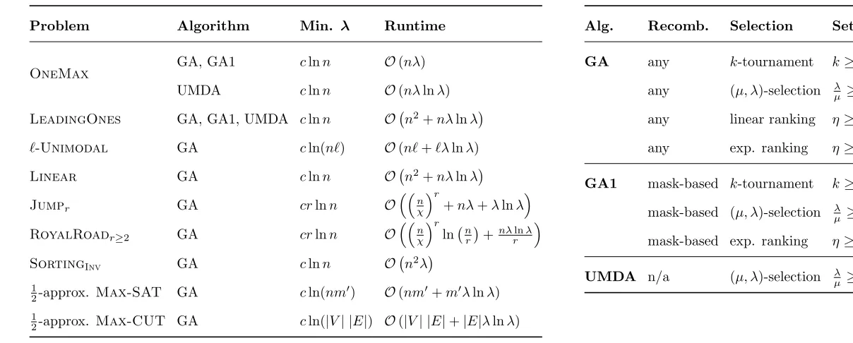
and provides upper bounds on the expected runtime for all these functions and classes.

Theorem 9. The expected runtime of the GA in Algorithm 2, withpc= 1−Ω(1)

using any crossover operator, a bitwise mutation with mutation rate χ/n for

any fixed constant χ > 0 and one of the selection mechanisms: k-tournament selection,(µ, λ)-selection, linear or exponential ranking selection, with their pa-rametersk,λ/µ andη being set to no less than(1 +δ)eχ/(1−pc)whereδ >0

being any constant, is

• O(nλ)onOneMax _ifλ≥clnn,

• O n2_+nλlnλ

on LeadingOnes_{if λ≥clnn,}

• O(nℓ+ℓλlnλ)onℓ-Unimodal _{ifλ≥cln(ℓn),}

• O n2_+nλlnλ

on Linear_{if λ≥clnn,}

• On

χ

r

+nλ+λlnλon Jump_{r ifλ≥crlnn,}

• On

χ

r

ln n_r

+nλ_rlnλ onRoyalRoad_{r≥2 if λ≥crlnn,}

for some sufficiently large constantc.

Proof. We apply Corollary 5 with the canonical partition Aj :={j |f(x) =j}

for all functions1_{, except forLinear, the fitness-based partition [16]:}

Aj:=

(

x_|

j

X

i=1

ci≤f(x)<

j+1

X

i=1

ci

)

forj_{∈ {}0_{} ∪}[n₋1] andAn:={1n}, is used.

The choices ofsj ands∗ to satisfy (M1) are the following.

1_{The first level can be}

A0instead ofA1for some functions but that does not matter as far

• ForOneMax_{, we set}

sj :=

_n

−j

1

_χ

n 1− χ n

n−1

= Ω _n −j n ,

i. e. the probability of flipping a 0-bit while keeping all the other bits unchanged, ands∗:= Ω _n1.

• ForLeadingOnes_,ℓ-Unimodal_andLinear_{, we set}

sj := χ

n

1−χ_nn−1= Ω

1

n

=:s∗,

i. e. the probability of flipping a specific bit to create a Hamming neighbour solution with better fitness while keeping all the other bits unchanged. In

ℓ-Unimodal_{, the bit to flip must exist by the definition of the function. In} LeadingOnes_{, the 0-bit at positionj+ 1 should be flipped. For}Linear_,

the partition satisfies that among the firstj+ 1 bits there must be at least a 0-bit, thus it suffices to flip the left most 0-bit will produce a search point at a higher level.

• ForJump_{r, as similar to}OneMax_{forj∈[n−1] we use}

sj :=

_n

−j+ 1 1

_χ

n 1− χ n

n−1

= Ω

_n

−j+ 1

n

,

butsn := χ_n r

1−χn

n−r

= Ω χ_nr

, i. e. the probability of flipping the

rremained 0-bits, sos∗:= Ω _n1

r

.

• ForRoyalRoad_{r, we use}

sj:=

n/r₋j

1

χ

n

r

1₋χ

n

n−r

= Ωχ

n

rn

r −j

,

i. e. the probability of flipping an entire unsolved block of lengthr(in the worst case) while keeping the other bits unchanged, ands∗:= Ω 1_n

r

. It follows from Lemma 19 that the probability of not flipping any bit position by mutation is (1₋χ/n)n

≥1₋₁₊δ/_δ/2₂e−χ ₌ e−χ

1+δ/2 forn sufficiently large,

thus choosingp0:= e

−χ

1+δ/2 satisfies (M2).

We now look at (M3). Ink-tournament selection, we have

k_≥ (1 +δ)e

χ

1₋pc

=

1 + δ/2 1 +δ/2

1 (1₋pc)p0

.

Hence, it follows from Lemma 7 that (M3) is satisfied with constantδ′_:= δ/2 1+δ/2.

The same conclusion can be drawn for the other three selection mechanisms. In (M4), sinceγ0andδ′are constants, there should exist a constantc >0 for

each function such that the condition is satisfied given the minimum requirement on population size related to c.

Since all conditions are satisfied, Corollary 5 gives the desired result for each function. For OneMax _and Jump_{r, optimisation time can be saved at early}

levels, i. e. sj is not small at the beginning, thus the evaluation of the sum

Pm−1

j=1 ln

6δλ

4+γ0sjδλ

• ForOneMax_{, simplifying each term by ln} 6

γ0sj

gives

O ln 6

n_nn

γn

0

Qn−1

j=0(n−j)

!!

=_O

ln

6n_nn

n!γn

0

,

and by Stirling’s approximation n! = Θ(nn+1

2/en), this is no more than

O(n). The expected runtime is then O(λn+nlnn). Since we already requireλ= Ω(lnn), this can be written shortly asO(nλ).

• ForJump_{r, we use the simplification ln} 6

γ0sj

for the first m₋2 terms of the sum, and ln(3λ/2) for the last term, so this gives

O ln 6

n_nn−1

γn

0

Qn−1

j=1(n−j+ 1)

!

+ lnλ

!

=O

ln

6n_nn

n!γn

0

+ lnλ

=_O(n+ lnλ).

The expected runtime is then_On χ

r

+nλ+λlnλ.

For the other functions,sj is already small at early levels, thus there is no

benefit of considering the gradual sum of ln. Hence, the simplificationO(mlnλ) for the sumPm−1

j=1 ln

6δλ

4+γ0sjδλ

gives the corresponding results.

In the case of regular use of crossover, i. e. pc = 1, the relationship

be-tween the crossover operator and the structure of the search space becomes non-negligible. In the following, we consider a generalmask-basedcrossover as follows. Given two parent genotypesu, v,the operator consists in first choosing (deterministically or randomly) a binary string ˜m = (m1, . . . , mn) to produce

two offspring vectorsx′_{, x}′′ _as

x′

i=

ui, if mi= 1

vi, otherwise, x

′′

i =

vi, if mi= 1

ui, otherwise.

Then one element of_{x′_{, x}′′

}chosen uniformly at random is returned. For exam-ple, the uniform crossover is a mask-based crossover for which ˜m_∼Unif(_{0,1_}n_),

and ak-point crossover is a mask-based crossover for which

˜

m_∼Unif

(

0a1₁a2₀a3_{. . .}

|ai∈N,

k+1

X

i=1

ai=n

)!

.

The following lemma shows that all mask-based crossover operators sat-isfy (C3) with ε= 1/2 for Om_andLo_functions.

Lemma 10. Ifx∼pxor(u, v), wherepxor is a mask-based crossover, then:

1. IfLo_{(u) =}Lo_{(v) =j, thenPr (}Lo_{(x)≥j) = 1,}

otherwisePr (Lo_(x)>min{Lo_(u),Lo_(v)})≥1/2.

Proof. 1) When Lo_{(u) =} Lo_{(v) = j, in mask-based crossover operators, the}

two bitstrings x′_{, x}′′ _{have j leading ones. So does the returned bitstring, i. e.}

with probability 1.

If Lo_{(u) 6=} Lo_{(v), we can assume w. o. l. g. that} Lo_{(v) = j and} Lo_{(u) >} Lo_{(v). Then v has a 0 while u has a 1 at position j+ 1. So, one of the}

bitstringsx′_,x′′ _{in the mask-based crossover will inherit the 1 at that position}

and the other will inherit the 0. This implies that one of them has fitness at leastj+ 1 and with probability 1/2 it is returned as output.

2) Each bit ofuandvis copied either tox′_{or tox}′′_{, therefore}

|x′

|1+|x′′|1=

|u|1+|v|1, which means that max{|x′|1,|x′′|1} ≥ ⌈(|u|1+|v|1)/2⌉. The output

is chosen with probabilities 1/2 to be copied either fromx′_orx′′_{, and the result}

follows.

Theorem 11. Assume that the GA in Algorithm 2 withpc= 1uses any

mask-based crossover operator, a bitwise mutation with mutation rate χ/n for any

fixed constantχ >0, and one of the following selection mechanisms: • k-tournament selection withk_≥8(1 +δ)eχ_,

• (µ, λ)-selection withλ/µ_≥2(1 +δ)eχ_{, or}

• exponential ranking selection withη_≥8(1 +δ)eχ_,

for any constant δ > 0. Then there exists a constant c > 0, such that the expected runtime of the GA is

• O(nλ)onOneMax _ifλ≥clnn,

• O n2_+nλlnλ

on LeadingOnes_{if λ≥clnn.}

Proof. We apply Corollary 6 this time, but again using the canonical partition of the search space for both functions. We also assume thatn is large enough so that by Lemma 19 the probability of not flipping any bit by mutation is (1₋χ/n)n

≥1₋₁₊δ/_δ/2₂e−χ ₌ e−χ

1+δ/2 =:p0, and so (C2) is satisfied with this

choice of p0. In addition, we use the same upgrades probabilitiessj and their

smallest value s∗ for each of the two functions as in the proof of Theorem 9 to

satisfy (C1).

It follows from Lemma 10 that (C3) is satisfied for constant ε1 := 1/2.

We now look at condition (C4). For k-tournament, we get k ≥ 8(1 +δ)eχ ₌

41 + ₁₊δ/_δ/2₂/(p0ε1). So condition (C4) is satisfied with constantδ′ := ₁₊δ/_δ/2₂

fork-tournament by Lemma 8. The same reasoning can be applied so that (C4) is also satisfied for the other selection mechanisms.

Sinceδ′_andγ

0are constants, thus condition (C5) is satisfied givenλ≥clnn

and for some constantc. Since all conditions are satisfied, the result follows from Corollary 6.

Note that the upper bounds in Theorem 11 match the upper bounds of Theorem 9. The latter is a generalisation of the results in [16] which were limited to EAs without crossover.

In the next sections, we further demonstrate the generality of Theorem 1 through Corollary 5 by deriving bounds on the expected runtime of GAs with

pc = 1−Ω(1) to optimise or to approximate the optimal solutions of

combi-natorial optimisation problems. We start with a simple problem of sorting n

4.2

Optimisation on permutation space

Given n distinct elements from a totally ordered set, we consider the problem of ordering them so that some measure of sortedness is maximised. Several measures were considered by [52] in the context of analysing the (1+1) EA. One of those is Inv_{(π) which is defined to be the number of pairs (i, j) such that}

1 ≤i < j ≤n, π(i)< π(j) (i.e. pairs in correct order). We show that with the method introduced in this paper, i. e. Corollary 5 analysing GAs on Sorting problem with Inv _{measure, denoted by} Sorting_{Inv, is not much harder than}

analysing the (1+1) EA.

For the mutation we use the Exchange(π) operator [52], which consecutively appliesN pairwise exchanges between uniformly selected pairs of indices, where

N is a random number drawn from a Poisson distribution with parameter 1.

Theorem 12. If the GA in Algorithm 2 withpc= 1−Ω(1)uses any crossover

operator, theExchange mutation operator, one of the selection mechanisms: k -tournament selection, (µ, λ)-selection, and linear or exponential ranking selec-tion, with their parametersk,λ/µandηbeing set to no less than(1+δ)e/(1₋pc),

then there exists a constantc >0 such that if the population size isλ_≥clnn, the expected time to obtain the optimum ofSorting_{Inv isO n}2_λ

.

Proof. Define m := n₂

. We apply Corollary 5 with the canonical partition,

Aj := {π | Inv(π) = j} for j = {0} ∪[m]. The probability that mutation

exchanges 0 pairs is 1/e. Hence, condition (M2) is satisfied forp0:= 1/e.

To show that (M1) is satisfied, we first define sj := m_em−j for each j ∈

{0_{} ∪}[m₋1]. Sincex_∈Aj, then the probability that the exchange operator

exchanges exactly one pair is 1/e, and the probability that this pair is incorrectly ordered in x, is (m₋j)/m. Thus, (M1) is satisfied with the definedsj.

In (M3), fork-tournament we have thatk≥(1+1−δp)ce=

1 + ₁₊δ/_δ/2_2(1−p1_c)p0, thus the condition is satisfied for constantδ′_:= δ/2

1+δ/2 and some constant γ0∈

(0,1) by Lemma 7. The same conclusion can be drawn be the other selection mechanisms. Finally, since γ0, δ′ are constants, there exists a constant c > 0

such that (M4) is satisfied for any λ_≥cln(n).

It therefore follows by Corollary 5 that the expected runtime of the GA on

SortingInv is O n2λ, i. e. this is similar to OneMax except that we have

m=O(n2_{) levels.}

4.3

Search for Local Optima