An extended branch and bound algorithm for linear bilevel programming

An Extended Branch and Bound Algorithm for Linear Bilevel

Programming

Chenggen Shi, Jie Lu and Guangquan Zhang Faculty of Information Technology

University of Technology, Sydney Sydney, NSW 2007, Australia {cshi, jielu&zhangg}@it.uts.edu.au

Hong Zhou*

Electrical, Electronic & Computing Engineering Faculty of Engineering & Surveying The University of Southern Queensland Toowoomba, Queensland 4350, Australia

[email protected]

Phone: 61 7 46311322, Fax: 61 7 46312526

An Extended Branch and Bound Algorithm for Linear Bilevel

Programming

Abstract

For linear bilevel programming, the branch and bound algorithm is the most successful algorithm to deal with the complementary constraints arising from Kuhn-Tucker conditions. However, one principle challenge is that it could not well handle a linear bilevel programming problem when the constraint functions at the upper-level are of arbitrary linear form. This paper proposes an extended branch and bound algorithm to solve this problem. The results have demostrated that the extended branch and bound algorithm can solve a wider class of linear bilevel problems can than current capabilities permit.

Keyword: linear bilevel programming, branch and bound algorithm, optimization, Von

1. Introduction

The game theory of Von Stackelberg [1] has motivated bilevel programming (BLP). In a basic BLP model, the upper-level is termed as the leader and the lower-level is termed as the follower. The leader goes first and attempts to optimize his/her objective function. The follower observes the leader’s decision and makes his/her decision. The majority of research on BLP has centered on the linear version of the problem. There have been nearly two dozen algorithms [2,3,4,5,6,7,8,9,10] proposed for solving linear BLP problems since the field being caught the attention of researchers in the mid-1970s.

This is how to solve a linear BLP problem when the upper-level’s constraint functions are in arbitrary linear form.

Our previous work presented a new definition of solution and related theorem for linear BLP, thus solved the fundamental deficiency of existing linear BLP theory [13]. In [14], we proposed an extended Kth-best approach for linear BLP. In [15], we completed theoretical foundation of Tucker approach and developed an extended Kuhn-Tucker approach. Based on these results, this paper develops an extended branch and bound algorithm for linear BLP. Following the introduction, this paper overviews linear BLP in Section 2. Deficiency of the branch and bound algorithm is addressed in Section 3. Section 4 presents an extended branch and bound algorithm. Numeric examples are given in Section 5. Section 6 gives a conclusion.

2. Linear bilevel programming

For x∈X ⊂Rn , y∈Y ⊂ Rm , F:X×Y →R1, and f :X×Y →R1 , a linear BLP problem is given by Bard [2]:

y d x c y x F

X

x ( , ) 1 1

min = +

∈ (1a)

subject to A₁x+B₁y≤b₁ (1b) f x y c x d y

Y

y ( , ) 2 2

min = +

∈ (1c)

subject to A2x+B2y≤b2, (1d) where c , ₁ n

R

c₂∈ , d , ₁ m

R

d₂∈ , p

R

b₁∈ , q

R

b₂∈ , p n

R

A₁∈ × , p m

R

B₁∈ × , q n

R A₂∈ × ,

m q

Let u∈Rq and v∈Rm be the dual variables associated with constraints (1d) and y≥0, respectively. Bard [2] gave the following proposition.

Proposition 1 A necessary condition that ( *, *)

y

x solves the linear BLP problem (1) is that there exist (row) vectors u and * v such that * (x*,y*,u*,v*) solves:

)

min(c1x+d1y (2a)

subject to A₁x+B₁y≤b₁ (2b)

uB2 −v=−d2 (2c)

u(b2 −A2x−B2y)+vy=0 (2d)

A2x+B2y≤b2 (2e)

x≥0,y≥0,u≥0,v≥0. (2f) Definition 1

A topological space is compact if every open cover of the entire space has a finite subcover. For example, [ ba, ] is compact in R (the Heine-Borel theorem) (http://thesaurus.maths.org/dictionary/map/word/10037 accessed 1 December 2003) Corresponding to (1), we gave following basic definition for linear BLP solution in [13]. Definition 2

(a) Constraint region of the linear BLP problem:

} ,

, , : ) ,

{(x y x X y Y A₁x B₁y b₁ A₂x B₂y b₂

S = ∈ ∈ + ≤ + ≤ .

The linear BLP problem constraint region refers to all possible combinations of choices that the leader and follower may make.

(b) Projection of S onto the leader’s decision space: } ,

, :

{ )

(X x X y Y A1x B1y b1 A2x B2y b2

Unlike the rules in noncooperative game theory where each player must choose a strategy simultaneously, the definition of BLP model requires that the leader moves first by selecting a x in attempt to minimize his objective subjecting to

both upper and lower level constraints. (c) Feasible set for the follower ∀x∈S(X): S(x)={y∈Y:(x,y)∈S}.

The follower’s feasible region is affected by the leader’s choice of x , and the follower’s allowable choices are the elements of S .

(d) Follower’s rational reaction set forx∈S(X): )]} ( ˆ : ) ˆ , ( min[ arg :

{ )

(x y Y y f x y y S x

P = ∈ ∈ ∈ ,

where argmin[f(x,yˆ):yˆ∈S(x)]={y∈S(x): f(x,y)≤ f(x,yˆ),yˆ∈S(x)}. The follower observes the leader’s action and reacts by selecting y from his feasible set to minimize his objective function.

(e) Inducible region:

)} ( , ) , ( : ) ,

{(x y x y S y P x

IR = ∈ ∈ .

The rational reaction set P(x) defines the response while the inducible region IR represents the set over which the leader may optimize his objective. Thus in terms of the above notations, the linear BLP problem can be written as

} ) , ( : ) , (

min{F x y x y ∈IR . (3) We presented and proved the following theorem to characterize the condition under which there is an optimal solution for a linear BLP problem in [13].

Theorem 1 If S is nonempty and compact, there exists an optimal solution for a linear

Let u∈Rp, v∈Rq and w∈Rm be the dual variables associated with constraints (1b), (1d) and y≥0, respectively. We presented and proved the following theorem in [15]. Theorem 2 A necessary and sufficient condition that ( *, *)

y

x solves the linear BLP problem (1) is that there exist (row) vectors u*, v*and w* such that (x*,y*,u*,v*,w*) solves:

y d x c y x

F( , ) _{1 1}

min = + (4a)

subject to A₁x+B₁y≤b₁ (4b)

A₂x+B₂y≤b₂ (4c)

uB₁+vB₂ −w=−d₂ (4d)

u(b₁−A₁x−B₁y)+v(b₂ −A₂x−B₂y)+wy=0 (4e) x≥0,y≥0,u≥0,v≥0,w≥0. (4f) 3. Deficiency of the branch and bound algorithm

In light of Proposition 1, Bard [12] proposed the branch and bound algorithm. This algorithm has been applied with remarkable success in linear bilevel programming, but its performance is dependent on linear form of the upper-level constraint functions. By using the following example, the deficiency is explored.

Example 1 Consider the following linear BLP problem with 1

R

x∈ , 1

R

y∈ , and }

0 { ≥

= x

X ,Y ={y≥0}.

y x y x F

X

x ( , ) 4

min = −

∈

f x y x y

Y

y∈ ( , )= +

min

subject to −2x+ y≤0 2x+y≤12.

Let us write down all the inequalities in the follower’s problem as: 0

2 ) , (

1 x y = x−y≥

g

0 12 2

) , (

2 x y =− x−y+ ≥

g

0 )

, (

3 x y = y≥

g .

By (3), we have

y x 4 min −

subject to −x−y≤−3 −3x+2y≥−4 −2x+ y≤0 2x+y≤12 u₁+u₂ −u₃ =−1

u1g1(x,y)+u2g2(x,y)+u3g3(x,y)=0 x≥0,y≥0,u₁ ≥0,u₂ ≥0,u₃ ≥0.

4. An extended branch and bound algorithm for linear bilevel programming Theorem 2 provides theoretical foundation for our new algorithm. The basic idea of our algorithm is following:

Write all the inequalities (except of the leader’s variables) of (1) as

m q p i

y x

g_i( , )≥0, =1,K, + + _{, and note that complementary slackness simply means} 0

) , (x y = g

ui i (i=1,K,p+q+m). Now we suppress the complementarity term and

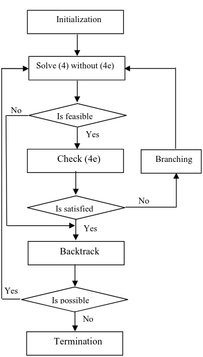
solve the resulting linear sub-problem. At each iteration, a check is made to see if (4e) is satisfied. If so, the corresponding point is in the inducible region and hence a potential solution to (1). If not, a branch and bound scheme is used to implicitly examine all combinations of complementarity slackness. A flowchart of the algorithm is displayed in Figure 3. The following notations are employed in the description of the algorithm.

0

1 2

0 3=

g

0 3=

u

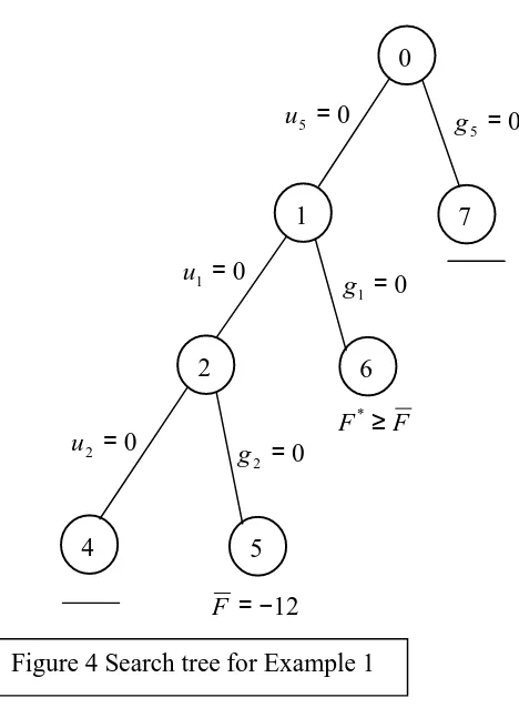
Figure 1 Search tree for Example 1

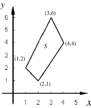
(1,2)

S

Figure 2 Geometry of linear BLP problem

x

(4,4) (3,6)

Let W ={1,K,p+q+m} _{be the index set for the terms in (4e), let F be the incumbent} upper bound on the leader’s objective function. At the kth level of the search tree we

define a subset of indices Wk ⊂W, and a path P corresponding to an assignment of k

either u_i =0 or g_i =0 for i∈W_k. Now let }

0 , :

{ ∈ =

= +

i k

k i i W u

S

} 0 , :

{ ∈ =

= −

i k

k i i W g

S

} :

{ 0

k

k i i W

S = ∉ .

Solve (4) without (4e)

Is feasible

Check (4e)

Is possible

Backtrack

Is satisfied Yes

Termination

No Yes

Branching No

Initialization

Figure 3 A flowchart of the extend branch and bound algorithm

Yes

For i∈Sk0, the variables u or i g are free to assume any nonnegative value in the i

solution of (4) with (4e) omitted, so complementary slackness will not necessarily be satisfied. Our algorithm can be accomplished with the following procedure.

Step 0 (Initialization) Set k =0, S_k+ =φ, S_k− =φ, 0 {1, , }

m q p

S_k = K + + _{, and F} =∞_. Step 1 (Iteration k) Set u_i =0 for i∈S_k+ and g_i =0 for i∈S_k−. Attempt to solve (4) without (4e). If the resultant problem is infeasible, go to Step 5; Otherwise, put k ←k+1 and label the solution ( k, k, k)

u y

x .

Step 2 (Fathoming) If F(xk,yk)≥F, go to Step 5. Step 3 (Branching) if ( k, k)=0

i k

i g x y

u , i=1,K,p+q+m_{, go to Step 4. Otherwise,}

select i for which ( k, k)≠0

i k

i g x y

u is the largest and label it i . Put ₁

S_k+ ←S_k+ ∪{i₁}, S_k0 ←S_k0 \{i₁}, S_k− ←S_k−, append i to ₁ P , and go to Step 1. _k

Step 4 (Updating) F ←F(xk,yk).

Step 5 (Backtracking) If no live node exists, go to Step 6. Otherwise branch to the newest live vertex and update S , k+

−

k

S , S and k0 P as discussed below. Go to k

Step1.

Step 6 (Termination) If F =∞, there is not feasible solution to (1). Otherwise, declare the feasible point associated with F the optimal solution to (1).

6 10−

<

i k i g

u it is considered to be zero. Confirmation indicates that a feasible solution of the bilevel program has been found and at Step 4 the upper bound on the leader’s objective function is updated. Alternatively, if the complementary slackness conditions are not satisfied, the term with the largest product is used at Step 3 to provide the branching variable. Branching is always done on the Kuhn-Tucker multiplier.

At Step 5, the backtracking operation is performed. Note that a live node is one associated with a sub-problem that has not yet been fathomed at either Step 1 due to infeasibility or at Step 2 due to bounding, and whose solution violates at least one complementary slackness condition. To facilitate bookkeeping, the path P in the branch _k

and bound tree is represented by a vector, its dimension is the current depth of the tree. The order of the components of P is determined by their level in the tree. Indices only k

appear in P if they are in either k

+

k

S or S with the entries underlined if they are in k−

−

k

S .

Because the algorithm always branches on a Kuhn-Tucker multiplier first, backtracking is accomplished by finding the rightmost non-underlined component if P , underlining it, _k

and erasing all entries to the right. The erased entries are deleted from S and added to _k−

0

k

S .

5. Numeric examples for the extended branch and bound algorithm Let us solve Example 1 to show how the extended branch and bound algorithm works. According to our algorithm, we have

0 3 )

, (

1 x y =x+y− ≥

g

0 4 2 3 ) , (

2 x y =− x+ y+ ≥

0 2

) , (

3 x y = x−y≥

g

0 12 2

) , (

4 x y =− x−y+ ≥

g

0 )

, (

5 x y = y≥

g ,

and also have

y x 4 min −

subject to −x−y≤−3 −3x+2y≥−4 −2x+ y≤0 2x+y≤12

−u1 −2u2 +u3 +u4 −u5 =−1

u₁g₁(x,y)+u₂g₂(x,y)+u₃g₃(x,y)+u₄g₄(x,y)+u₅g₅(x,y)=0 x≥0,y≥0,u1 ≥0,u2 ≥0,u3 ≥0,u4 ≥0,u5 ≥0.

Finally we get following linear programming problem with one check condition.

y x 4 min −

subject to −x−y≤−3 −3x+2y≥−4 −2x+y≤0 2x+y≤12

−u1 −2u2 +u3 +u4 −u5 =−1

At each iteration, the check is made to see if the following condition is satisfied. u1g1(x,y)+u2g2(x,y)+u3g3(x,y)+u4g4(x,y)+u5g5(x,y)=0.

More specifically, after initializing the data, the algorithm finds a feasible solution to the Kuhn-Tucker representation with the complementary slackness conditions omitted and proceeds to Step 3. The current point, x1 =3 , y1 =6 , u1 =(0,0,0,0,1) , with

21 ) ,

(x1 y1 =−

F does not satisfy complementarity so a branching variable is selected )

(u₅ and the index sets are updated, giving S₁+ ={5}, S₁− =φ , S₁0 ={1,2,3,4} and }

5 { 1 =

P . In the next two iterations, the algorithm branches on u and ₁ u , respectively. ₂

Now, three levels down in the tree, the current sub-problem at Step 1 turns out to be infeasible so the algorithm goes to Step 5 and backtracks. The index sets are S₃+ ={5,1},

} 2 { 3 =

−

S , S₃0 ={3,4} and P₃ ={5,1,2}. Go to Step 1, a feasible solution is found. It passes the test at Step 2 and satisfied the complementary slackness conditions at Step 3. Continuing at Step 4, F =−12. The algorithm backtracks at Step 5 and updates the sets,

} 5 { 4 =

+

S , S₄− ={1}, S₄0 ={2,3,4} and P₄ ={5,1}. Returning Step 1, another feasible solution is found, but at Step 2, the value of the leader’s objective function is greater than the incumbent upper bound, so the algorithm goes to Step 5 and backtracks, giving

φ

= +

5

S , S₅− ={5}, S₅0 ={1,2,3,4} and P₅ ={5}. The current sub-problem at Step 1 turns out to be infeasible so the algorithm goes to Step 5 and backtracks. However, no live vertices exist. we have found an optimal solution, occurring at the point ( *, *)=(4,4)

y x , ) 0 , 0 , 0 , 5 . 0 , 0 ( ) , , , ,

Example 2 Consider the following linear BLP problem with 1

R

x∈ , 1

R y∈ , and }

0 { ≥

= x

X ,Y ={y≥0}.

y x y x F X

x ( , ) 2

min = −

∈

subject to f x y x y

Y

y∈ ( , )= +

min

subject to −x+3y≤8

x−y≤0 .

By using both the current branch and bound algorithm and extended branch and bound algorithm, we have

0 8 3 ) , (

1 x y =x− y+ ≥

g

0 )

, (

2 x y =−x+ y≥

g 12 − = F F F*≥

0 2 = u ₀ 2 = g 0 1 2 4 6 5 7 0 1 = g 0 5 = g 0 1 = u 0 5 = u

0 )

, (

3 x y =y≥

g

y x 2 min −

subject to −x+3y≤8 x−y≤0

3u₁ −u₂ −u₃ =−1

u₁g₁(x,y)+u₂g₂(x,y)+u₃g₃(x,y)=0 x≥0,y≥0,u1 ≥0,u2 ≥0,u3 ≥0.

By using the same way as that of previous one, we have found an optimal solution, occurring at the point ( *, *)=(4,4)

y

x , ( , , *) (0,1,0) 3

* 2 *

1 u u =

u with * =−4

F and * =8

f . This result is again identical with that in [13].

The results have demostrated that the extended branch and bound algorithm for linear BLP can solve a wider class of problems than current capabilities permit.

6. Conclusion

The fundamental deficiency of current branch and bound algorithm is that it could not well solve a linear BLP problem when constraint functions at the upper-level are of arbitrary linear form. This paper presents an extended branch and bound algorithm for linear BLP to deal with this issue. The performance comparisons have demostrated that a wider class of problems can be solved by using the extended branch and bound algorithm.

References

1 Von Stackelberg H (1952). The Theory of the Market Economy. Oxford

University Press: York, Oxford.

2 Bard J (1998). Practical Bilevel Optimization: Algorithms and Applications.

Kluwer Academic Publishers: USA.

3 Candler W and Townsley R (1982). A linear two-level programming problem. Computers and Operations Research 9: 59-76.

4 Bialas W and Karwan M (1984). Two-level linear programming. Management Science 30: 1004-1020.

5 Bard J and Falk J (1982). An explicit solution to the multi-level programming problem. Computers and Operations Research 9: 77-100.

6 Bialas W and Karwan M. Multilevel linear programming. Technical Report 78-1,

1978, State University of York at Buffalo.

7 Hansen P, Jaumard B, and Savard G (1992). New branch-and-bound rules for linear bilevel programming. SIAM Journal on Scientific and Statistical Computing 13:1194-1217.

8 Bialas W, Karwan M and Shaw J. A parametric complementary pivot approach for two-level linear programming. Technical Report 80-2, 1980, State University

of York at Buffalo.

10 White D and Anandalingam G (1993). A penalty function approach for solving bi-level linear programs. Journal of Global Optimization 3: 397-419.

11 Fortuny-Amat J and McCarl B (1981). A representation and economic interpreta-tion of a two-level programming problem. Journal of the Operational Research Society 32: 783-792.

12 Bard J and Moore JT (1990). A branch and bound algorithm for the bilevel programming problem. SIAM Journal on Scientific and Statistical Computing 11:

281-292.

13 C. Shi, G. Zhang, and J. Lu, "On the definition of linear bilevel programming solution," Applied Mathematics and Computation, vol. 160, pp. 169-176, 2005.

14 C. Shi, J. Lu, and G. Zhang, "An extended Kth-best approach for linear bilevel programming," Applied Mathematics and Computation, vol, 164, 843-855.

15 C. Shi, J. Lu, and G. Zhang, "An extended Kuhn-Tucker approach for linear bilevel programming," Applied Mathematics and Computation, vol. 162, pp.