University of Southern Queensland Faculty of Engineering and Surveying
Internal Model Control (IMC) of a Fruit Drying
System
A dissertation submitted by
Scott A. Geddes
in fulfilment of the requirement of
Courses ENG4111 and 4112 Research Project
towards the degree of
Bachelor of Engineering (Computer Systems)
Abstract
The use of automation within the food processing industry, has allowed for the continual improvement in production and quality control, including that for dried fruit products.
By monitoring and controlling process variables within a commercial fruit dryer (dehydrator), quality control features such as moisture-content, texture, and colour etc, can be attained. The three minimum process variables within most commercial fruit dryers to achieve successful drying are air-temperature, air-velocity, and relative-humidity.
This project investigates the control of air-temperature in a fruit dehydrator by firstly implementing a PID controller. Then as a separate exercise, an IMC controller is implemented, and a performance comparison between the PID and IMC controllers was conducted.
The PID controller was initially designed using the Ziegler-Nichols (step response method), but was determined to be too inaccurate for this purpose. So optimization using Steepest Descent Minimization was also used to determine the PID controller gains.
IMC being considered a robust adaptive controller [6], is especially suited to this plant, having both a large time-constant and transport-delay.
Determining an IMC controller for this process involved, first obtaining the process inverse (non-linear transport-lag term ignored), then designing a low-pass filter with the filter parameter being the only parameter requiring tuning in the entire IMC control system.
University of Southern Queensland Faculty of Engineering and Surveying
ENG4111 & ENG4112
Research Project
Limitations of Use
The council of the University of southern Queensland, its Faculty of Engineering and Surveying, and the staff of the University of Southern Queensland, do not accept any responsibility for the truth, accuracy or completeness of material contained within or associated with this dissertation.
Persons using all or any part of this material do so at their own risk, and not at the risk of the Council of the University of Southern Queensland, its Faculty of Engineering and Surveying or the staff of the University of Southern Queensland.
This dissertation reports an educational exercise and has no purpose or validity beyond this exercise. The sole purpose of the course pair entitled “Research Project” is to contribute to the overall education within the student’s chosen degree program. This document, the associated hardware, software, drawings, and other material set out in the associated appendices should not be used for any other purpose: if they are so used, it is entirely at the risk of the user.
Prof R Smith Dean
Certification
I certify that the ideas, designs, experimental work, results, analyses and conclusions set out in this dissertation are entirely my own effort, except where otherwise indicated and acknowledged.
I further certify that the work is original and has not been previously submitted for assessment in any other course or institution, except where specifically stated.
Scott Geddes
Student Number: Q82405374
Signature
Acknowledgments
I am grateful to Dr. Paul Wen for his valuable comments and suggestions throughout this project and during the preparation of this dissertation.
Scott Geddes
University of Southern Queensland
Contents
Abstract ... i
Certification ...iv
Acknowledgments ... v
Contents ...vi
List of Figures...ix
List of Tables ... xiii
Notation...xiv
List of Terms...xv
chapter 1 ... 1
Introduction... 1
1.1 Introduction... 1
1.2 Project Aim ... 2
1.3 Dissertation Structure ... 3
chapter 2 ... 6
Fruit Drying Modelling... 6
2.1 Introduction... 6
2.2 The parameters modelled ... 6
2.2.1 Relative Humidity... 7
2.2.2 Air Speed... 8
2.2.3 Air Temperature... 8
2.3 Batch or Continuous Flow... 9
2.4 Parallel, Counter or Cross Flow ... 10
chapter 3 ... 12
The Fruit Dryer Plant Model... 12
3.1 Introduction... 12
3.2 The general fruit dryer model... 12
3.3 The numerical fruit dryer model ... 14
3.4 The open-loop plant transfer function of the fruit dryer... 16
PID Temperature Control for the Fruit Drying Plant ... 17
4.1 Introduction... 17
4.2 PID Controller Review ... 17
4.3 PID control of temperature... 20
4.4 Ziegler-Nichols (step-response method) ... 20
4.5 PID Temperature Controller Simulation ... 22
4.6 Optimization Theory... 25
4.7 Optimization of PID gains ... 27
4.7.1 Frequency response of the optimized PID system ... 28
4.8 Simulation of the PID controlled fruit dryer system... 29
4.8.1 PID – Simulation of varying plant transport delays. ... 30
4.8.2 PID – Simulation of varying plant time-constants. ... 31
4.8.3 PID - Unit step disturbance at the plant output. ... 33
4.8.4 PID - Unit pulse disturbance at the plant output. ... 34
4.8.5 PID - Band limited white noise disturbance at the plant output. 35 4.9 PID Conclusion... 37
chapter 5 ... 38
Internal Model Control (IMC) Theory... 38
5.1 IMC Introduction ... 38
5.2 IMC System Theory ... 38
5.3 IMC General System Design ... 40
5.3.1 IMC Controller Design... 43
5.3.2 IMC Filter Design ... 43
5.3.3 IMC Time Delay Compensation ... 44
5.3.4 IMC Sensitivity and Complementary Sensitivity ... 45
chapter 6 ... 47
IMC Temperature Control for the Fruit Drying Plant... 47
6.1 Introduction... 47
6.2 Numerical IMC controller design ... 48
6.2.1 Numerical IMC filter design. ... 49
6.3 Implementing the IMC controller for the fruit dryer. ... 52
6.4 Simulation of the IMC fruit dryer system ... 54
6.5 IMC Plant model mismatch of transport delays ... 56
6.6 IMC - Plant model mismatch of time-constants ... 58
6.7 IMC – Unit step disturbance at the plant output ... 61
6.8 IMC – Unit pulse disturbance at the plant output... 62
6.9 IMC – Band limited white noise disturbance at the plant output. 63 6.10 Conclusion... 65
chapter 7 ... 66
PID/IMC Evaluation and Comparison ... 66
7.1 Introduction... 66
7.2 Performance comparison criteria ... 66
7.3 PID and IMC comparison... 66
7.3.1 PID controlled system. ... 66
7.3.2 IMC controlled system. ... 67
chapter 8 ... 70
Conclusions and Future Work... 70
8.1 Conclusions ... 70
8.2 Future Work... 70
References ... 71
Appendix A ... 73
Appendix B ... 74
List of Figures
FIGURE 3-1 TYPICAL FRUIT DRYER SHOWING THERMAL SCHEMATIC OF THE
PLANT...13
FIGURE 3-2 SYSTEM MODEL OF THE OPEN-LOOP THERMAL TRANSFER FUNCTION OF THE PLANT...14
FIGURE 4-1 PID CLOSED LOOP SYSTEM IMPLEMENTATION...20
FIGURE 4-2 OPEN LOOP STEP RESPONSE OF THE PROCESS...21
FIGURE 4-3 PID CONTROLLER IMPLEMENTATION...22
FIGURE 4-4 RESPONSE OF OPEN-LOOP SYSTEM TO A 1V STEP INPUT...23
FIGURE 4-5 PID PARAMETERS FOR ZIEGLER-NICHOLS STEEPEST DESCENT METHOD...24
FIGURE 4-6 STEP INPUT RESPONSE USING ZN PID CONTROLLER PARAMETERS. ...24
FIGURE 4-7 PID CONTROLLER IMPLEMENTATION...25
FIGURE 4-8 SYSTEM MODEL FOR PLANT TRANSPORT DELAY T =12...27
FIGURE 4-9 PID CONTROLLER PARAMETERS OBTAINED FROM OPTIMIZATION.27 FIGURE 4-10 RESPONSE USING OPTIMIZED PID CONTROLLER PARAMETERS..28 FIGURE 4-11 FREQUENCY RESPONSE USING OPTIMIZED PID CONTROLLER PARAMETERS...29
FIGURE 4-12 MODEL CONSIDERED WITH VARYING PLANT TRANSPORT DELAY VALUES Td...30
FIGURE 4-13 PID STEP RESPONSE TO VARYING PLANT TRANSPORT DELAY FROM Td =12 TO Td =6 (IN STEPS OF 3 SECONDS)...31
FIGURE 4-14 MODEL CONSIDERED WITH VARYING PLANT TIME-CONSTANT VALUES
τ
...32FIGURE 4-15 PID MODEL STEP RESPONSE TO VARYING PLANT TIME-CONSTANT, VALUES
τ
SECONDS...32FIGURE 4-16 PID MODEL FOR A UNIT STEP DISTURBANCE AT THE PLANT OUTPUT...33
DEGREES CELSIUS...34
FIGURE 4-18 PID MODEL FOR A UNIT PULSE DISTURBANCE AT THE PLANT OUTPUT...34
FIGURE 4-19 PID MODEL RESPONSE TO A UNIT PULSE DISTURBANCE OF 1 DEGREES CELCIUS...35
FIGURE 4-20 PID MODEL OF A BAND LIMITED WHITE NOISE DISTURBANCE AT THE PLANT OUTPUT...35
FIGURE 4-21 SIMULATION OF BAND LIMITED WHITE NOISE DISTURBANCE SOURCE...36
FIGURE 4-22 PID MODEL RESPONSE TO A BAND LIMITED WHITE NOISE DISTURBANCE SOURCE...37
FIGURE 5-1 OPEN-LOOP CONTROL SYSTEM...39
FIGURE 5-2 IMC CONTROL SYSTEM...40
FIGURE 6-1 IMC SYSTEM IMPLEMENTATION (
τ
f =0.5)...50FIGURE 6-2 RESPONSE OF SYSTEM TO A UNIT STEP INPUT (
τ
f =0.5)...51FIGURE 6-3 BODE RESPONSE TO THE ABOVE RANGE OF DELAYS (
τ
f =0.5)...51FIGURE 6-4 IMC SYSTEM IMPLEMENTATION FOR THE FRUIT DRYER (
τ
f =1.5). ...54FIGURE 6-5 RESPONSE OF IMC SYSTEM FOR THE FRUIT DRYER WITH NO PLANT/MODEL MISMATCHES OR DISTURBANCES (
τ
f =1.5)...55FIGURE 6-6 MISMATCH OF TRANSPORT-DELAYS (Tp =11.6,
Tm=12)...56
FIGURE 6-7 RESPONSE BEFORE COMPENSATING (Tp=11.6,
Tm =12)...57
FIGURE 6-9 COMPENSATED RESPONSE FOR A MISMATCH OF TRANSPORT
DELAYS (Tp =11.6,
Tm =11.6)...58
FIGURE 6-10 PLANT, PLANT MODEL MISMATCH OF TIME-CONSTANTS (
τ
p =12,τ
m =10)...59FIGURE 6-11 RESPONSE BEFORE COMPENSATING, (
τ
f =1.5,τ
m =10)...59FIGURE 6-12 COMPENSATED PLANT/MODEL MISMATCH OF TIME-CONSTANTS (
τ
p =12,τ
m =12)...60FIGURE 6-13 RESPONSE OF COMPENSATED SYSTEM (
τ
p =12,τ
m=12)...61FIGURE 6-14 IMC MODEL FOR A UNIT STEP DISTURBANCE...61
FIGURE 6-15 IMC RESPONSE TO A UNIT STEP DISTURBANCE...62
FIGURE 6-16 IMC MODEL TO A UNIT PULSE DISTURBANCE...62
FIGURE 6-17 IMC RESPONSE TO A PULSE DISTURBANCE...63
FIGURE 6-18 IMC MODEL FOR A BAND LIMITED WHITE NOISE DISTURBANCE...64
List of Tables
TABLE 2-1 MAXIMUM DEHYDRATOR TEMPERATURES USING FULL
DEHYDRATION...9
TABLE 3-1 TRANSPORT DELAY TIME FOR A PARTICULAR FAN SETTING...15
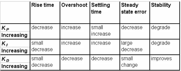
TABLE 4-1 EFFECTS OF INDEPENDENTLY TUNING GAIN VALUES IN
CLOSED-LOOP SYSTEM...19
TABLE 4-2 PID PARAMETERS FOR ZIEGLER-NICHOLS STEP RESPONSE METHOD.
Notation
D
distance between heat source and thermostat [m]( )
P
G s
process transfer function PK proportional gain I
K integral gain D
K derivative gain
L transport delay approximation using ZN (step response method) R steepest gradient using ZN (step response method)
T general transport delay [s]
m
T model transport delay [s]
p
T plant transport delay [s]
τ
plant time-constant [s]f
τ
filter time-constant [s]air
V
air velocity between heat source and thermostat [m/s]s
derivative transfer functionList of Terms
continuous dryer: Dryer which dries fruit continuously on a conveyor, or rack rail system (as opposed to a batch dryer which needs to be load/unload fruit directly to/from the dryer).
decay ratio: The ratio of maximum amplitudes of successive oscillations.
dead time: (see transport delay).
finish dehydration: The drying of fruit is conducted in a mechanical dehydrator that has first been partly dried in the sun (sun-dried). The sun-drying component improves the colour of many products (whilst not forget, moisture is also being removed by less expensive sun-drying).
full dehydration: The drying of fruit is conducted in a mechanical dehydrator from the fresh (wet) state to completion, ready for packaging (often results in poor colour).
overshoot: The magnitude by which the controlled variable swings past the setpoint.
plant: The air in the drying chamber of the fruit dryer (dehydrator).
rise time: The time the response takes to comes up to the new setpoint.
robustness: The system should not be overly sensitive to changes in process parameters.
settling time: The time it takes the amplitude of the oscillations to decay to some fraction of the change in setpoint.
tunnel dryer: see continuous dryer.
transport delay: Time delay between two processes in a system model.
chapter 1
Introduction
1.1 Introduction
Dried tomatoes, apples, figs, sultanas, and also rice, beans (including coffee) and many spices are only a handful of the dried fruit products available to the consumer today. Fruit by definition is the reproductive part of any edible seed plant; yet, consumers of dried fruit usually refer to only any sweet tasting dried plant product as being fruit including for example banana and ginger (which by strict definition is not a fruit). For this reason the term dried fruit in this dissertation refers to any plant, or part of that plant in its dried form.
Historically, many cultures throughout the world have developed methods to dry fruit for; food preservation, culinary pleasure, and medicinal use. But by far sun drying has been the most popular method, although simple kiln arrangements were used for certain seasonal fruits, especially for those harvested in colder climates, and during times of bad weather. In many parts of the world these methods are still practised today.
A popular method of drying is finish dehydration. The fruit is first sun dried until a certain moisture content and colour is obtained, then the fruit is then placed in the dehydrator for the remainder of the time required. As fruit dries, the internal moisture becomes increasingly difficult to remove; and it is at this later stage of drying that the dehydrator can be of most value.
temperature, air-velocity, relative humidity, thus the total drying regime. Some dehydrators have the ability to monitor parameters in real time such as, specimen size/depth, specimen moisture content, colour etc within the drying environment, to provide real-time feedback to the control parameters (providing a drying regime of quality consistency for different types and sizes of fruit).
One fundamental problem using dehydrators is that, for many fruits the dehydrator cannot give the fruit that authentically sundried appearance demanded by the market. Future research into the application of artificial light (UV) in the drying process may fill this gap in dehydrator technology.
1.2 Project Aim
The aim of this project was to design, simulate, and test a PID controlled system to control temperature for a given plant, then, using this exact same transfer function of the plant, an Internal Model Control (IMC) controlled system model was also investigated, and compared to the PID model.
The fruit dryer process was modelled as a transfer function consisting of a temperature gain term, first order lag term, with a transport delay term. The design of a controller for this process shall consider the following criteria:-
• the system must always be stable and bounded.
• a fast response for this system is not required.
• it must reach setpoint within 60 seconds with less than 5% overshoot at any time.
• the system must be robust enough to control the process model errors and disturbances.
1.3 Dissertation Structure
This dissertation is divided into the following chapters.
Chapter 2: Fruit Drying Modelling
An introduction is given to the types of fruits which are dried, and the parameters that are used to dry them. This chapter also discusses how these parameters interact with each other, and how they must be modelled in a control system to achieve successful drying.
Chapter 3: The Fruit Dryer Plant Model
The temperature model of the fruit dryer plant is obtained to allow for simulations of the system in subsequent chapters, and achieve accurate control of this process.
Chapter 4: PID Temperature Control of the Fruit Drying Plant
The theory of the PID controller is briefly outlined, and then control of the fruit drying plant using the PID is implemented. Plant/plant model mismatches and disturbances are simulated.
Chapter 5: Internal Model Control (IMC) Theory
This chapter provides the theory of IMC. The theory warrants an entire chapter since much of chapter 6 where the IMC controller is implemented numerically, assumes complete knowledge of the reader to the material of chapter 5.
Chapter 6: IMC Temperature Control of the Fruit Drying Plant
Chapter 7: PID/IMC Evaluation and Comparison
An evaluation of the significance of the responses of the PID and IMC systems is conducted then a comparison is made between the performances of both systems.
Chapter 8: Conclusions and Future Work
chapter 2
Fruit Drying Modelling
2.1 Introduction
Recent advances in fruit drying technology have led to the development of new methods and techniques to dry fruit, including the use of microwave, infra-red, and U.V. radiation to provide the drying energy [7]. Yet today, drying is still mostly achieved, by placing the fruit in a controlled environment of increased air-temperature and air-flow, and low humidity.
Commercial fruit dryers (mechanical dehydrators) are designed to provide a consistent, quality assured finished product, and a steady production cycle of dried fruit during all weather and seasons. A disadvantage of many dehydrators is that they fail to provide the colour of their ‘sundried’ counterparts (that the market demands). One solution being developed is a combination of initial UV light application (simulating sundrying) followed then by the insertion into the dehydrator, this can have considerable advantages without the loss of fruit quality.
2.2 The parameters modelled
During the second phase of drying, the rate of moisture loss decreases. The second phase begins when the rate of moisture movement to the surface of the fruit is less than the rate of evaporation from the surface. That is, the speed of drying is limited by the rate at which moisture can move through the fruit tissue. These principles also apply to drying using more traditional means, such as sun-drying.
Under mechanical dehydration the overall speed of drying depends on the relative humidity, and the speed and temperature of air passing over the fruit. These parameters need to be monitored and controlled throughout, and inattention to any of them can jeopardise the success of the entire process.
2.2.1 Relative Humidity
Relative humidity control is the most important factor for efficient dehydration. Air in a dehydrator continually circulated without replacement would rapidly become saturated with water vapour. Evaporation would stop and the fruit would begin to 'cook'.
To avoid this it is necessary to 'bleed off' some of the moist air and replace it with dry air from outside. The aim is to keep the relative humidity below approximately 40%. It must be done carefully because if too much air is bled off with little or no recirculation, heating costs can be extremely high. A compromise must be made between full discharge of partly saturated air (maximum drying rate) and full recirculation of saturated air (minimum heat use).
moisture to be removed. As the fruit dries, further moisture is more difficult to remove and maintenance of a low relative humidity level becomes less important. However, in this second stage of the drying process, the relative humidity of air should still be kept below 40%. Relative humidity of the air is measured before it has passed through the heating unit and fan and after the fruit stack.
2.2.2 Air Speed
The movement of air has two essential functions in the drying of fruit. It transfers heat from the heating device to the fruit (to provide the energy required to vaporise the water). Secondly, it serves as a vector for the moisture to be transferred from inside the dehydrator to the outside atmosphere.
Air speeds of 3 to 5 m/s are recommended for fruit dehydration. Speeds above 6 m/s are used for certain heat sensitive fruits, but these speeds are usually uneconomical because of the much greater power needed to drive the fan.
Air speed is most important in the initial stages of full dehydration when free water is present on the surface of the fruit. Under these conditions the drying rate is doubled when the airspeed is increased. Less attention need be paid to airspeed in the later stages of drying or when using finish dehydration, but airspeed of less than 3.0 m/s can slow the drying rate. Dehydrators designed with a fixed airspeed of 3.4 m/s over the fruit circulate a sufficient volume of air to provide heat for both evaporation and the removal of moisture from the unit for most fruits.
2.2.3 Air Temperature
Air temperature is increased to supply the heat required to evaporate fruit moisture and to increase the moisture-carrying capacity of the air.
cold air, a relatively small volume of hot air is needed to carry moisture out of the dehydrator. Additional heat is necessary to heat trays, compensate for heat lost through insulation, and heat the fresh air required to maintain a low humidity.
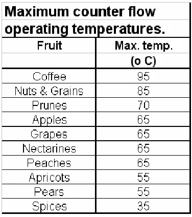
[image:26.612.225.413.220.432.2]The maximum operating temperature is determined by the temperature at which discolouration and off flavours is produced in the fruit (see below).
Table 2-1 Maximum dehydrator temperatures using full dehydration.
2.3 Batch or Continuous Flow
The dehydrator can be worked either as a batch system, or a continuous flow system.
In the batch system the dehydrator is filled with fruit and run until the entire load is dried to the desired moisture content. Another complete batch is then loaded, and the cycle repeated.
start of the dehydrator until it is full (or almost full). Then, when the first truck has dried sufficiently it is removed from the finish, and another put in at the start, and so on. This method is recommended for finish-drying stone fruits and pears.
A problem with the batch system is uneven rates of moisture removal from the fruit at different locations throughout the dehydrator. That is to say, fruit closest to the fan and heat source shall become dry quickest whilst microclimates near corners and badly sealed doors may be slower. For these reasons, at the completion of drying in a batch system there is a gradient in fruit moisture content from low at one end of the dehydrator to high at the other end.
Another problem associated with the batch system is the continual adjustment of shutters required to control relative-humidity during the drying cycle. This problem can be overcome with automatic relative-humidity control. An automated system allows the dehydrator to be operated overnight without supervision.
In contrast, in a continuous flow system, some fruit must be loaded and unloaded periodically while the dehydrator is operating, requiring labour around the clock. This regular removal and replacement of fruit to and from the dehydrator results in some extra heat loss when the doors are opened. A special truck and rail system are essential for efficient operation and to minimise energy losses. As the trucks of fruit are removed and reloaded periodically, the labour required for placing and removing fruit from the trays is spread out, as is the requirement for fresh fruit when using a continuous flow system.
2.4 Parallel, Counter or Cross Flow
chapter 3
The Fruit Dryer Plant Model
3.1 Introduction
Monitored parameters such as air-temperature, air-speed and humidity would typically be only the minimum parameters monitored. The drying regime for a fruit, that is, for different species, different size/thicknesses etc, are all controlled by adjusting air-temperature, air-speed and humidity during a prescribed time regime. Although some dehydrators have the ability to monitor these and other variables in real time such as, moisture-content, color etc, allowing for the specimen characteristics to dictate the drying regime, and not just simply a drying time.
Although a modern commercial fruit dryer may provide the means to control and monitor all these variables within a drying chamber, this project shall be limited to the control and monitoring of the dryer’s air-temperature only.
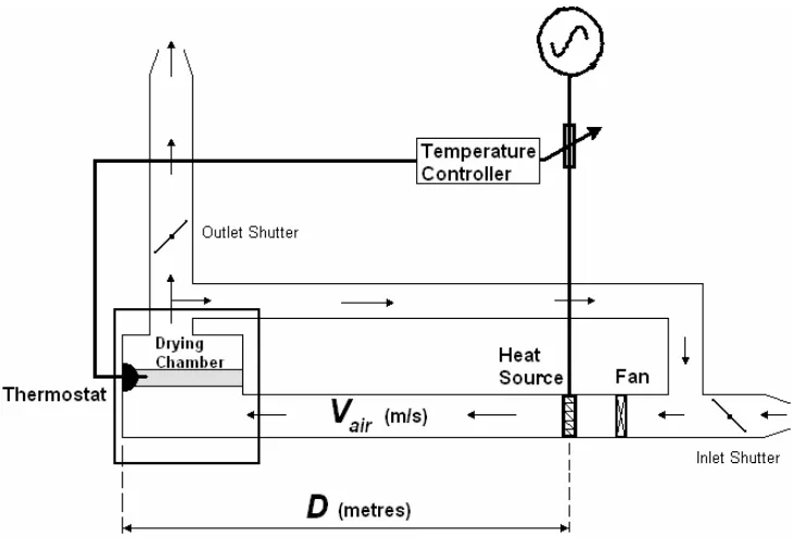
3.2 The general fruit dryer model
Figure 3-1 Typical fruit dryer showing thermal schematic of the plant.
The fruit drying process above was modelled by:
• a first-order lag term for the heat source (heater banks),
• a delay term acting between the heater banks and the drying chamber,
• an inverse gain term for the air temperature in the drying chamber (the air in the drying chamber was simply assumed to be a linear multiple of the heater-bank elements temperature),
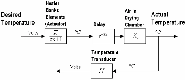
Figure 3-2 System model of the open-loop thermal transfer function of the plant.
The open-loop transfer function is then be represented by:
1 2 1 2 ( ) ( ) 1 ( ) ( ) 1 P P Ts D s Vair
K K H
G s H s e
s
K K H
G s H s e
s
τ
τ
− − = + ∴ = +3.3 The numerical fruit dryer model
This system was a 24V system, and was designed with H =1/ 5. So if 1V was applied to the input of the controlled closed-loop system, then there was a temperature of 5 degrees Celsius at the output. Thus our dryer’s upper temperature limit was 120 degrees Celsius. The feedback term not only provided feedback, but also provided a temperature to voltage conversion.
reach a steady state value when the open-loop system was provided with a step input.
It was assumed in our model that the air temperature in the drying chamber was 20% of the heater bank element’s temperature. So a value of K2=0.2 was simply chosen to model the air temperature in the drying chamber.
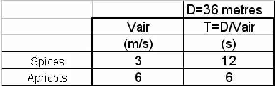
The value for D is small, in small modular fruit dryers that are available, but a larger food manufacturer providing ‘hot-air’ to many areas of the factory floor could typically have the heat source positioned larger distances away from the drying chamber. So an arbitrary value for the distance between the heat source and the thermostat was made to beD=36metres.
[image:32.612.179.462.417.506.2]Recall from the previous chapter where the minimum and maximum air speeds used for drying fruit was 3 m/s and 6 m/s respectively. Therefore using the table below as an example we can determine the transport-delay times for when the fan speed is set for a particular type of fruit.
Table 3-1 Transport delay time for a particular fan setting.
3.4 The open-loop plant transfer function of the fruit
dryer
So our open-loop plant transfer function for minimum and maximum transport-delay is respectively:
6 12
36
30 0.2 0.2 ( ) ( )
10 1
1.2 1.2
( ) ( ) ( ) ( )
10 1 10 1
P s s P P air s V
G s H s e
s
e e
G s H s and G s H s
chapter 4
PID Temperature Control for the
Fruit Drying Plant
4.1 Introduction
The aim of this chapter is to detail the design, then simulate a PID controller for the temperature system model of the fruit dryer.
The tuning parameters shall be obtained, then system responses shall be recorded observing certain design objectives (for later comparison with the IMC input/output responses).
4.2 PID Controller Review
Controllers based on the PID design algorithm remain the most popular due to their inherent ability to converge to a solution for most linear (and many non-linear) applications, for a large given domain of inputs, and/or initial values. The ability for a PID system to perform with stability, with low (or zero) transient and steady state errors, depends on the accurate selection of the tuning parameters KP, KI,
( )
( )
( )
( )
( )
( )
( )
( )
0 0 1 1 ( ) ( ) t P tP I D
P I D
d i
d
u t K e t e t d e t
dt
d
u t K e t K e t d K e t
dt
U s E s K K K s
s
τ τ
τ
τ
= + + = + + = + + ∫
∫
where: u t( ) = controller output (and the total error)
( )
e t = desired value – measured value
P
K , KI, and KD are the respective error term gains.
To allow the controller to be designed within a stable system criterion, these three error gain terms will determine the response of the closed-loop system to inputs and initial conditions by the following action:
• provide control action via proportionality to the error, implemented using an all-pass gain factor.
• reducing steady-state errors via low-frequency compensation, implemented using an integrator.
• improving transient response via high-frequency compensation, implemented using a differentiator.
Controller parameters are tuned such that the closed-loop control system is always stable and should meet given objectives associated with the following:
• stability, robustness.
• steady-state error performance.
[image:36.612.139.500.181.323.2]• disturbance rejection from load surges, plant/model uncertainties, environmental noise.
Table 4-1 Effects of independently tuning gain values in closed-loop system.
For given objectives, tuning techniques for PID controllers can be categorized into two general methods according to their application as follows:
• Analytical methods Tuning parameters are calculated from an analytical or algebraic relation between the plant model and an objective (eg. IMC) needs to be in an analytical form and the model must remain extremely accurate. Real-time automated tuning would be included in this method.
• Heuristic methods Manual tuning/programming (such as the Ziegler-Nichols tuning rules) or from an artificial intelligence base in the form of a neural network rule/formulae).
parameters to produce many different improved responses to the system.
4.3 PID control of temperature
The open-loop plant was now transformed into a closed loop system, with the addition of feedback and a PID controller. Two methods were investigated to determine whether they could provide accurate temperature setpoint tracking, within a reasonably fast response time for the dryer, without compromising stability of the system. They were, the Ziegler-Nichols (step-response method), and optimization of the PID coefficients using a steepest descent minimization algorithm.
Figure 4-1 PID closed loop system implementation.
4.4 Ziegler-Nichols (step-response method)
as ours):
( )
1
Ts
Ke G s
s
τ
−
= +
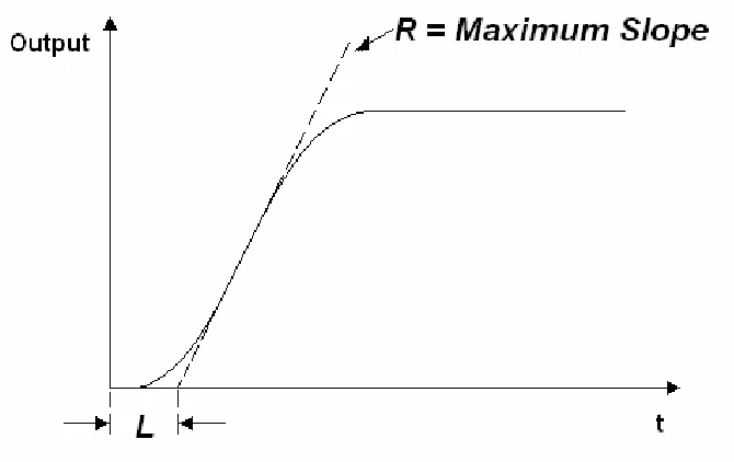
[image:38.612.152.487.209.420.2]This process has a general open-loop step response below:
Figure 4-2 Open loop step response of the process. To design the controller from this output the following steps are taken:
• determine the steepest gradient R.
• determine the delay term L.
Table 4-2 PID parameters for Ziegler-Nichols step response method.
• then the gain terms are substituted into in the controller equation,
( )
P I 1 D ( )U s K K K s E s
s
= + +
• U s
( )
is the controlled input signal to the plant, it is this signal which determines the output Y s( )
in the closed-loop system as follows:Figure 4-3 PID controller implementation.
4.5 PID Temperature Controller Simulation
fruit drying process was considered to be one of the most popular open-loop responses encountered in industry.
To design the PID controller for the fruit drying process we shall follow the steps outlined in the previous section as follows:
• obtain the open-loop step response below:
Figure 4-4 Response of open-loop system to a 1V step input.
• the steepest gradient term was determined to be 6
48
R= (although choosing the numerator term was difficult since there was a high degree of discretion due to the curvature of the response).
• the delay term L=12.
Figure 4-5 PID parameters for Ziegler-Nichols steepest descent method.
A simulation of the closed-loop system was conducted with the above determined controller gain values:
0 20 40 60 80 100 120
0 1 2 3 4 5 6
Temperature vs Time
Time (s)
T
e
m
p
e
ra
tu
re
Figure 4-6 Step input response using ZN PID controller parameters.
the system to reach steady-state sooner. Also the slope R near the time-axis can be too large for visual judgement (or other graphical means of estimation), which when implemented allows for inaccurate gain control action to occur, thus a slower time to reach set-point.
4.6 Optimization Theory
Optimization allowed us to tune the PID parameters by a more accurate criterion required by the system. In this case the specifications of the controller were to disallow overshoot above 5%, but still reach steady state within the required 60 seconds.
The optimization technique used here shall be the steepest decent minimization method from [1] (p. 4.12). The system details and numerical calculations are contained in the source code in appendix B, but a general discussion of this method shall be given here.
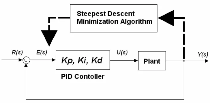
[image:42.612.137.501.416.597.2]Below is the model being simulated to determine PID controller gains:
An initialization of PID parameters (see code Appendix B) was chosen, and then the response to a step input was simulated. The simulated error value E(s), is tested against the IAE (Integral Absolute Error) criteria, which forces a magnitude increase/decrease of the respective PID controller gains.
The IAE performance criteria used to obtain these minimum values shall be:
0 ( ) T IAE=
∫
e t dtAnd the general algorithm to implement steepest descent minimization shall be:
[
]
0min min T ( )
Optimized System= IAE = e t dt
∫
Steepest descent minimization searches for a minimum slope. An initial value is chosen, simulated, substituted into an objective function, and then the magnitude of this objective function is compared with the previously simulated value. The minimum value is chosen for the next iteration, whilst the maximum of the two is rejected.
In more detail, steepest descent minimization uses the surface variable S in say 3 dimensions x, y, z (but could use higher dimensionality), where the gradient of S
is:
ˆ
ˆ ˆ
S S S
S i j k
x y z
∂ ∂ ∂ ∇ = + +
∂ ∂ ∂
This method searches using its objective function in the direction of negative gradient −∇S . Initial values x(0), (0), (0)y z are chosen then iteratively run through following formulae:
( 1) ( ) ( )
( 1) ( ) ( )
( 1) ( ) ( )
x
y
z
x k x k S k
y k y k S k
z k z k S k
(where
η
is the normalized step size)If there is proportionality to the negative gradient−∇S, then the (k+1) iteration replaces the (k) iteration. If there is not proportionality to−∇S, then the (k) iteration is simply retained (see source code appendix B).
4.7 Optimization of PID gains
The following system model was optimized.
Figure 4-8 System model for plant transport delay T =12.
After optimization of the system (see appendix B for source code used) the following PID controller parameters were obtained and a simulation using these values was conducted.
The response of the system using the above optimized PID controller parameters is shown below.
Figure 4-10 Response using optimized PID controller parameters. The system did not reach our specified setpoint in under 60 seconds. It displayed approximately 10% overshoot initially, but had a high enough damping to eliminate oscillatory behaviour within approximately 80 seconds.
Two other choices were then considered at this stage, to use a system with less damping, or use an optimized PI controller instead. The higher damped system overcame the overshoot problem but did not solve the problem of reaching set-point within specifications when disturbances were considered later. The optimized PI controller had a similar problem meeting overshoot specifications (specified as 5%). So a decision was made to implement the PID controlled system with this overshoot compromised.
4.7.1 Frequency response of the optimized PID system
As the transport-delay increases, its phase margin usually decreases, indicating that the system is becoming less stable (or unstable). If there is a decrease in the transport-delay this usually increases the phase margin and can indicate that the system is becoming more stable.
Figure 4-11 Frequency response using optimized PID controller parameters.
The system was stable with a comfortable Pm=63.9 degrees, and the use of a PID compensator was not required. This robustness needed to be established before accurate responses to disturbances could be evaluated, and also a stable robust PID system can only be properly compared with a stable robust IMC controller later.
4.8 Simulation of the PID controlled fruit dryer system
To fully test the PID controlled system, the following change in plant parameter values and other external disturbance simulations were independently conducted:
2. A change in the plant, due to a change plant time-constant values. 3. Unit step disturbance at the plant output.
4. Pulse disturbance in at the plant output. 5. White noise disturbance at the plant output.
4.8.1 PID – Simulation of varying plant transport delays.
For systems requiring robustness to changes in transport delay capabilities, this is not usually where the application the PID controllers have their best reputation. Although our fruit dryer model was designed using the value of Td =12 seconds to fully consider the effects of simulated drifts in transport delay values, smaller transport delay times are considered, using the following model.
Figure 4-12 Model considered with varying plant transport delay values d
T .
Using now the model of the original transfer function with Td =12, then observe below the response due to incremental changes in the transport delay Td, stepping down from Td =12 to Td =6 in steps of 3 seconds (this is simulating
air
Figure 4-13 PID step response to varying plant transport delay from
12
d
T = to Td =6 (in steps of 3 seconds).
As the transport delay was decreased, the response experienced more damping with a much slower rise time, but fell short of reaching set point within 60 seconds but did not display any instability. Although when Td >12 the system quickly experiences large values of overshoot.
For every fan setting (ie
V
air), that is, for every transport delay value, it would be required to complete the optimization of their respective PID parameters, and use those PID parameters for that particularV
air setting. This would be a formidable task if the sensitivity of the system required the optimization of PID parameters at many time steps to achieve the desired accuracy.4.8.2 PID – Simulation of varying plant time-constants.
Figure 4-14 Model considered with varying plant time-constant values
τ
.To illustrate this, a simulation was made whereby our modelled plant time-constant value of
τ
=10seconds (original designed system), was varied fromτ
=8 toτ
=14 (values chosen wereτ
= 8,10, &14 ). These values forτ
were chosen to not cause more than 10% overshoot in the response (see response below).As expected a reduction in the time-constant to
τ
f =8 allowed higher frequency components to enter the system which was not intended for in the controller design forτ
f =10, and overshoot and a more oscillatory system resulted.Values higher than
τ
f =14 increase overshoot and damping but neither of these disturbances reaches setpoint within 60 seconds.4.8.3 PID - Unit step disturbance at the plant output.
Simulating disturbances at summing junctions is not a multiplicative process, thus a better understanding of the magnitudes in the response of the system shall be gained by using the full system (non-normalized). This practise shall be adopted for all simulated disturbances at summing junctions in this dissertation.
Figure 4-16 PID model for a unit step disturbance at the plant output.
Figure 4-17 PID model response to a unit step disturbance of 1 degrees Celsius.
4.8.4 PID - Unit pulse disturbance at the plant output.
attributes of a stable, robust system:
Figure 4-19 PID model response to a unit pulse disturbance of 1 degrees Celcius.
4.8.5 PID - Band limited white noise disturbance at the
plant output.
Figure 4-20 PID model of a band limited white noise disturbance at the plant output.
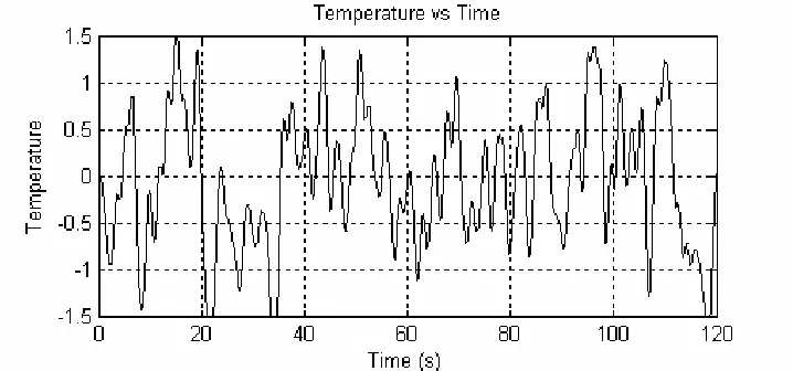
[image:52.612.144.501.419.547.2]disturbance (as was the case with the step and pulse disturbances) may not be adequate.
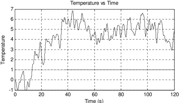
[image:53.612.141.500.247.415.2]A stochastic disturbance model in the form of a band limited white noise source shall be used to simulate unknown disturbances of this kind. The output of the random disturbance subsystem is shown below. It comprises a sinusoid with variable amplitude and frequency (the low-pass filter cut off frequency was 2 rad/s (0.32 Hz)).
0 20 40 60 80 100 120 -1 0 1 2 3 4 5 6 7
Temperature vs Time
[image:54.612.159.474.96.277.2]Time (s) T e m p e ra tu re
Figure 4-22 PID model response to a band limited white noise disturbance source.
4.9 PID Conclusion
This chapter discussed the theory of the PID controller, the implemented PID controller design of the temperature controller of our fruit drying plant. To determine PID parameters The ZN (steepest decent method) was first used but proved to be too inaccurate, and the IAE Optimization method was used.
chapter 5
Internal Model Control (IMC)
Theory
5.1 IMC Introduction
The IMC controller is a model based controller, and is considered to be robust. Mathematically, robust means that the controller must perform to specification, not just for one model but for a set of models [2]. The IMC controller design philosophy adheres to this robustness by considering all process model errors as bounded and stable (including transport lag differences between the model and the physical system). IMC is implemented by firstly obtaining the inverse of the process (or invertible components of it) to be controlled, then multiplying this calculated inverse with a low-pass filter. The output response to the reference inputs, the sensitivity function and the complementary sensitivity function can be adjusted directly by the low-pass filter [8].
5.2 IMC System Theory
Figure 5-1 Open-loop control system.
Let G sp( ) be a model of G sp( ), and
let 1
( ) ( )
c p
G s =G s − (ie the controller is the inverse of the process model),
then G sp( )=G sp( ) (ie an exact representation of the process).
This theoretical control performance whereby the output remains equal to the input (or setpoint), without the use of feedback, informs us of two things:
• assuming we have complete knowledge of the process
(encapsulated in the process model) being controlled, then perfect control can be achieved.
• feedback is only necessary when knowledge about the process is inaccurate or incomplete.
Both these above conditions in practise are unachievable in an open-loop system, for the following reasons:
• a mismatch between the actual process, and the process model.
• the process model may not be invertible.
• unknown disturbances within the system.
5.3 IMC General System Design
[image:57.612.140.539.144.317.2]Below is the general IMC system design [6]:
Figure 5-2 IMC control system.
The output, Y s( ), is compared with the output of the process model, resulting in signal d s( ) below,
( ) p( ) p( ) ( ) ( )
d s =G s −G s U s +d s
If d s( )=0, then, d s( ) is a measure of the difference in behaviour between the process and its model.
If G sp( )=G sp( ), then d s( )=d s( ),
Then d s( ) is used to subtract from the setpoint R s( ) here below,
( ) ( ) ( ) c( )
U s =R s −d s G s
( ) ( ) p( ) p( ) ( ) ( ) c( )
U s =R s −G s −G s U s +d s G s
[
( ) ( )]
( )( )
1 ( ) ( ) ( )
c
p p c
R s d s G s U s
G s G s G s
− =
+ −
Substitute U s( ), into output Y s( ) below,
( ) p( ) ( ) ( )
Y s =G s U s +d s
to obtain the closed-loop expression below,
[
( ) ( )]
( ) ( )( ) ( )
1 ( ) ( ) ( )
c p
p p c
R s d s G s G s
Y s d s
G s G s G s
−
= +
+ −
( ) ( ) ( ) 1 ( ) ( ) ( )
( )
1 ( ) ( ) ( )
c p c p
p p c
G s G s R s G s G s d s
Y s
G s G s G s
+ − = + − Eqn 5.3-1
If G sc( )=G sp( )−1 and,
If G sp( )≠G sp( ), zero error disturbance rejection can be achieved, provided that
1
( ) ( )
c p
G s =G s − .
To improve robustness, the effects of mismatch between the process, and process model should be minimised. Since the differences between process and the process model usually occur at the systems high frequency response end, a low-pass filter Gf(s) is usually added to attenuate this effect. Thus IMC is
designed using the inverse of the process model in series with a low-pass filter, ie:
( ) = ( ) ( )
IMC c f
G s G s G s
1
( ) = ( ) ( )
IMC p f
G s G s − G s Eqn 5.3-2
(where G sp( ) =−1 G sc( ), and where the order of the filter being usually
chosen such that G sp( )−1G sf( ) is proper (ie the highest numerator power is always less than the denominator’s), to disallow excessive differential control action)
Then substituting Eqn 5.3-2 into Eqn 5.3-1 to obtain an expression which includes the GIMC( )s term below:
( ) ( ) ( ) 1 ( ) ( ) ( )
( )
1 ( ) ( ) ( )
IMC p IMC p
p p IMC
G s G s R s G s G s d s
Y s
G s G s G s
5.3.1 IMC Controller Design
The process model G sp( ), must first be factored into invertible and non-invertible components, that is:
( ) ( ) ( _ )
p
G s = invertable
× non invertable
( ) ( ) ( )
p p p
G s =G + s ×G − s Eqn 5.3-4
The non-invertible component Gp−( )s , contains terms which if inverted, will lead to instability and realisability problems, ie terms containing positive zeros and time-delays (that were previously not there).
Then using ONLY the invertible component of the process model, let
1
( ) ( )
c p
G s =G + s − Eqn 5.3-5
and then substituting into
( ) ( ) ( )
IMC c f
G s =G s ×G s , then
1
( ) ( ) ( )
IMC p f
G s =G + s − ×G s Eqn 5.3-6
5.3.2 IMC Filter Design
(where
τ
f is the filter time constant, and n is the order of the filter (and the relative difference between the numerator and denominator, GIMC( )s is said to be proper if n=1). As a rule of thumbτ
f , can be chosen to at be at least twice as fast (up to 20 times as fast) as the open-loop response [8], but another method of choosingτ
f is using the following formulae:1
( ) (0) lim
20 (0) ( )
f
n n
s
D s N s D N s
τ
→∞
≥
whereD s( )andN s( )are taken from the following equation:
( ) ( ) ( )
p p p
G s =G + s ×G − s where ( ) ( ) ( ) p N s G s D s + =
5.3.3 IMC Time Delay Compensation
Examining the output of the close-loop system by letting G sp( )=G sp( ), then substituting Eqn 5.3-6 into Eqn 5.3-3 to get,
1 1
( ) ( ) ( ) ( ) ( ) 1 ( ) ( ) ( ) ( )
( ) ( ) ( ) ( ) 1 ( ) ( ) ( )
( ) ( ) 1 ( )
1 1
p p f p p f
p f p f
Ts Ts
f f
Y s G s G s G s R s G s G s G s d s
Y s G s G s R s G s G s d s
e e
Y s R s d s
s s
τ
τ
+ − + − − − − − = + − ∴ = + − ∴ = + − + + Thus, we can see that the IMC scheme has the following properties:
• it provides time-delay compensation
• the filter can be used to shape both the setpoint tracking and disturbance rejection responses.
5.3.4 IMC Sensitivity and Complementary Sensitivity
The Sensitivity function will be used as in [9], to specifically see the consequences of the controller design in IMC, and then briefly compared to the controller in a classical control system.
Since,
( ) ( )
( ) ( ) ( )
Y s E s
Sensitivity
d s R s d s
= = −
and from Eqn 5.3-3, let
( ) ( ) ( ) Y s s d s
ε
=1 ( ) ( )
( ) ( )
( ) 1 ( ) ( ) ( )
IMC p
IMC p p
G s G s
Y s s
d s G s G s G s
ε
= = −
+ −
Eqn 5.3-8
again substituting G sp( )=G sp( ) into Eqn 5.3-9 above to get,
( )s 1 GIMC( )s G sp( )
ε
= − Eqn 5.3-9( )s GIMC( )s G sp( )
η
= Eqn 5.3-101 ˆ( )
1 C( ) P( )
s
G s G s
ε
=+
( ) ( )
ˆ( )
1 ( ) ( )
C P
C P
G s G s s
G s G s
η
=+
chapter 6
IMC Temperature Control for the
Fruit Drying Plant
6.1 Introduction
The theory of IMC control introduced in the previous chapter shall now be implemented to control the temperature of the fruit drying plant. The fruit drying plant was especially suited for IMC control since:
• The system was open-loop stable (open loop response plot shown in chapter 3).
• IMC provided time delay compensation since there existed a delay in the process transfer function (between the time the heat from the heater banks is applied, to the time the thermostat in the drying chamber sensed this applied change).
6.2 Numerical IMC controller design
The design of the IMC controller implemented the theory from the previous chapter by determining the following:
1. a process model that was an exact representation of the process.
2. the inverse of the process model.
3. the filter parameter.
An exact process model representation was simply that of the open-loop process:
( ) ( ) 6 ( ) 5(10 1) p p p Ts
G s G s
e G s s − = ∴ = +
Then using only the invertible term of the process model (ie ignore the time delay term) below: 1 ( ) ( ) 5(10 1) ( ) 6 c p c
G s G s
s G s − + = + ∴ =
This was then substituted into the IMC controller below:
1 ( ) ( ) ( ) ( ) ( ) ( ) 5(10 1) ( ) ( ) 6
IMC c f
IMC p f
IMC f
G s G s G s
G s G s G s
s
G s G s
6.2.1 Numerical IMC filter design.
Before we can determine G sf( ) we first must determine
τ
f:1
1 1
1
( ) (0) lim
20 (0) ( )
5(10 1) 6
lim
20 5 6
10 1 lim 20 1 lim 0.5 20 0.5 f f n n s s s s
D s N s D N s
s s s s s
τ
τ
→∞ →∞ →∞ →∞ ≥ + × ≥ × × + ≥ ≥ + ≥This value of
τ
f =0.5 was then substituted into G sf( ) below(
)
(
)
1 ( ) 1 1 ( ) 0.5 1 f n f f G s s G s sτ
= + ∴ = + Eqn 6.2-2Therefore substituting Eqn 6.2-1 into Eqn 6.1-1 we obtained the IMC controller to be:
5(10 1) 1
( )
6 0.5 1
IMC s G s s + = +
Figure 6-1 IMC system implementation (
τ
f =0.5).0 10 20 30 40 50 60 0 1 2 3 4 5 6 Time (s) T e m p e ra tu re
Temperature vs Time
[image:68.612.163.472.105.272.2]Delay=6 Delay=12 Delay=18 Delay=24
Figure 6-2 Response of system to a unit step input (
τ
f =0.5).-1 -0.5 0 M a g n itu d e ( d B )
10-2 10-1 100
-720 -540 -360 -180 0 P h a s e ( d e g ) Bode Diagram
Gm = 0.0178 dB (at 0.128 rad/sec) , Pm = Inf
Frequency (rad/sec)
Figure 6-3 Bode response to the above range of delays (
τ
f =0.5). [image:68.612.163.470.364.525.2]value.
6.2.2 Numerical IMC considering different delays.
Since the delay term e−12s was omitted from the derivation of the controller
( )
IMC
G s (when plant transfer functions of the form of our G sp( ) are designed for), the controller for our system with transport-delay of 6 seconds e−6s (for drying apricots) would have exactly the same GIMC( )s . In fact we can set the delay to whatever value we choose.
This allows us to simply say ‘set’ the delay for 6 seconds (for drying apricots) or ‘reset’ the delay for 12 seconds (for drying spices), or any delay value in between, depending on the fruit we are drying. (In practise this set/reset process would be automatically conducted by an instrument to monitor
V
air to provide us these delay values). Recall our linear model for transport delay is simplyair
D T
V
= .
If we make changes to the supply ducting, or our distance D metres changes between heater-banks and drying chamber, that cause changes in transport delay, our controller remains essentially the same (assuming the plant remains the same of course).
6.3 Implementing the IMC controller for the fruit dryer.
Although we could have used this calculated minimum value of
τ
f =0.5 (which would provide the system with the fastest response time without instability), a value ofτ
f =1.5 was chosen to in fact increase the time to reach setpoint temperature in the un-delayed system from approximately 2.5 seconds to approximately 7.5 seconds.assumed that the time-constant of the instrument monitoring
V
air was less than 0.05 second, (allowing for the mismatch to be compensated for well within 0.5 second).This selection of
τ
f was justified, based on the rule of thumb where “τ
f can be chosen to be at least twice as fast as the open-loop response” [8]. According to this rule the time constant of the open-loop system is 10 seconds thereforeτ
f <(10 / 2).( )
f
G s (acting as a low pass filter) with its amended value of
τ
f, is shown below:(
)
1 ( ) 1.5 1 f G s s =+ Eqn 6.3-1
Therefore substituting Eqn 6.2-1 into Eqn 6.1-1 we obtained the amended IMC controller which was implemented in our fruit dryer system:
5(10 1) 1
( )
6 1.5 1
IMC s G s s + = +
Figure 6-4 IMC system implementation for the fruit dryer (
τ
f =1.5).6.4 Simulation of the IMC fruit dryer system
A simulation of this system (with T=12 seconds) using this controller was firstly conducted with no plant model matches, and no disturbances, that is with
( ) 0
0 10 20 30 40 50 60 0 1 2 3 4 5 6 Time (s) T e m p e ra tu re
Temperature vs Time
[image:72.612.162.473.96.262.2]Tp=Tm=12 seconds
Figure 6-5 Response of IMC system for the fruit dryer with no plant/model mismatches or disturbances (
τ
f =1.5).But further investigation was conducted about the IMC design to see whether it can be robust enough to resist plant model mismatch and other external disturbances. And, still reach a steady state, offset free response within 60 seconds. To fully address each disturbance individually, the following plant model mismatch/disturbance simulations were independently conducted for the T=12 second system (note: a different transport-delay value apart from T=12 seconds could have been chosen instead for this analysis).
6.5 IMC Plant model mismatch of transport delays
In our fruit dryer, once our fan speed has been set for spices (3 m/s) the transport-delay is then 12 seconds. This fan speed would be kept as constant as possible by a separate controller to the temperature controller, but forms an integral part or the transport delay value used in the plant model.
To realistically consider changes in the value of
V
air it was assumed that the maximum transport-delay time tolerance which could occur in this system without compensatory action occurring was 0.4 seconds. So when we simulated a plant model mismatch of transport-delays, the maximum difference between the plant transport-delay and the plant model transport delay allowed was 0.4 seconds. [image:73.612.134.506.425.579.2]To simulate a change in value of the plant transport delay, Tp was decreased from Tp =12 to Tp =11.6 whilst Tm remained at Tm =12, the system model and its response is shown below.
0 10 20 30 40 50 60 0
1 2 3 4 5 6
Time (s)
T
e
m
p
e
ra
tu
re
Temperature vs Time
[image:74.612.164.471.105.272.2]Output Y(s)
Figure 6-7 Response before compensating (Tp =11.6,
Tm =12).
To compensate for this plant model mismatch, Tm must be made to equal Tp again to adhere to the IMC philosophy of requiring that the plant model must be an exact representation of the plant. Below is shown the system model and response after this compensatory action has occurred.
[image:74.612.135.505.411.569.2]0 10 20 30 40 50 60 0 1 2 3 4 5 6 Time (s) T e m p e ra tu re
Temperature vs Time
[image:75.612.162.474.105.272.2]Output Y(s)
Figure 6-9 Compensated response for a mismatch of transport delays (Tp =11.6,
Tm =11.6).
A system whereby Tp drifted in value above Tm could have also been examined, except the uncompensated system would display overshoot instead of undershoot (as in the figure above), but the compensation strategy would be the same.
We could have also simulated a similar mismatch of plant and plant model transport-delays for any plant transport-delay value, and the controller remains the same, thus output responses remain the same except translated along the time axis.
It is for these reasons that systems requiring robustness to changes in transport delay capabilities are usually where IMC controllers find their most suitable applications.
6.6 IMC - Plant model mismatch of time-constants
value. Or at some stage there may be a physical alteration made to the plant that may cause a sudden change in plant’s time-constant that needs to be identified and compensated for. To illustrate this compensation a plant model mismatch of the time-constants where the plant time-constant increased from 10 seconds (original system) to 12 seconds is shown below:
Figure 6-10 Plant, plant model mismatch of time-constants (
τ
p =12,τ
m=10).0 10 20 30 40 50 60
0 1 2 3 4 5 6
Time (s)
T
e
m
p
e
ra
tu
re
Temperature vs Time
Y(s), Taup=10 Y(s), Tau
[image:76.612.157.477.320.568