Methodology for the Integration of Optomechanical System Software Models with a Radiative Transfer Image Simulation Model

(1)

Rochester Institute of Technology

RIT Scholar Works

Theses

7-12-2019

Methodology for the Integration of

Optomechanical System Software Models with a

Radiative Transfer Image Simulation Model

Keegan S. McCoy

(2)

Methodology for the Integration of Optomechanical System Software

Models with a Radiative Transfer Image Simulation Model

by

Keegan S. McCoy

B.S. in Electrical Engineering, The Pennsylvania State University, 2012 B.S. in Astronomy and Astrophysics, The Pennsylvania State University, 2012

M.S. in Electrical Engineering, The Pennsylvania State University, 2012

A dissertation submitted in partial fulfillment of the requirements for the degree of Doctor of Philosophy in the Chester F. Carlson Center for Imaging Science

College of Science

Rochester Institute of Technology

July 12, 2019

Signature of the Author

Accepted by

(3)

CHESTER F. CARLSON CENTER FOR IMAGING SCIENCE COLLEGE OF SCIENCE

ROCHESTER INSTITUTE OF TECHNOLOGY ROCHESTER, NEW YORK

CERTIFICATE OF APPROVAL

Ph.D. DEGREE DISSERTATION

The Ph.D. Degree Dissertation of Keegan S. McCoy has been examined and approved by the dissertation committee as satisfactory for the

dissertation required for the Ph.D. degree in Imaging Science

Dr. John Kerekes, Dissertation Advisor

Dr. Alan Raisanen, External Chair

Dr. Michael Gartley

Dr. Scott Rohrbach

Date

(4)

Methodology for the Integration of Optomechanical System Software

Models with a Radiative Transfer Image Simulation Model

by

Keegan S. McCoy

Submitted to the

Chester F. Carlson Center for Imaging Science in partial fulfillment of the requirements

for the Doctor of Philosophy Degree at the Rochester Institute of Technology

Abstract

Stray light, any unwanted radiation that reaches the focal plane of an optical system,

re-duces image contrast, creates false signals or obscures faint ones, and ultimately degrades

radiometric accuracy. These detrimental effects can have a profound impact on the

us-ability of collected Earth-observing remote sensing data, which must be radiometrically

calibrated to be useful for scientific applications. Understanding the full impact of stray

light on data scientific utility is of particular concern for lower cost, more compact imaging

systems, which inherently provide fewer opportunities for stray light control. To address

these concerns, this research presents a general methodology for integrating point spread

function (PSF) and stray light performance data from optomechanical system models in

optical engineering software with a radiative transfer image simulation model. This

in-tegration method effectively emulates the PSF and stray light performance of a detailed

system model within a high-fidelity scene, thus producing realistic simulated imagery. This

novel capability enables system trade studies and sensitivity analyses to be conducted on

parameters of interest, particularly those that influence stray light, by analyzing their

quan-titative impact on user applications when imaging realistic operational scenes. For Earth

(5)

iv

science applications, this method is useful in assessing the impact of stray light performance

on retrieving surface temperature, ocean color products such as chlorophyll concentration or

dissolved organic matter, etc. The knowledge gained from this model integration also

pro-vides insight into how specific stray light requirements translate to user application impact,

which can be leveraged in writing more informed stray light requirements.

In addition to detailing the methodology’s radiometric framework, we describe the

col-lection of necessary raytrace data from an optomechanical system model (in this case,

using FRED Optical Engineering Software), and present PSF and stray light component

validation tests through imaging Digital Imaging and Remote Sensing Image Generation

(DIRSIG) model test scenes. We then demonstrate the integration method’s ability to

pro-duce quantitative metrics to assess the impact of stray light-focused system trade studies

on user applications using a Cassegrain telescope model and a stray light-stressing coastal

scene under various system and scene conditions. This case study showcases the stray light

images and other detailed performance data produced by the integration method that take

into account both a system’s stray light susceptibility and a scene’s at-aperture radiance

profile to determine the stray light contribution of specific system components or stray

light paths. The innovative contributions provided by this work represent substantial

im-provements over current stray light modeling and simulation techniques, where the scene

image formation is decoupled from the physical system stray light modeling, and can aid

in the design of future Earth-observing imaging systems. This work ultimately establishes

an integrated-systems approach that combines the effects of scene content and the

optome-chanical components, resulting in a more realistic and higher fidelity system performance

(6)

v

DISCLAIMER

(7)

vi

The light shines in the darkness,

and the darkness has not overcome it.

(8)

Acknowledgements

First and foremost, I would like to thank God for standing by me not just during my time

in this rigorous Ph.D. program, but throughout my entire life. You provide me with the

strength to meet all of life’s challenges and I pray that I can continue to use the talents that

you have provided me for your glory. Though a doctorate degree is the pinnacle of academic

achievement, the more I learn about you and the world you have created, the more humble

I become.

I would like to thank my wife for her incredible amount of love and support. Though my

Ph.D. diploma has my name on it, you have been just as integral a part of the effort. Being

a military spouse is not easy in general, but this is especially true during a time-intensive

Ph.D. program in which we experienced life-altering changes, both joyful and tragic. You

have been a steady presence throughout it all and I look forward to sharing more of life’s

many adventures with you as we move on from our time in Rochester. I also apologize for

teaching you more about stray light and optical system modeling and simulation than you

probably ever care to know.

I would like to thank my parents, grandparents, and the rest of my family for their love

and encouragement not only during this Ph.D. program, but from the moment I was born.

I have been truly blessed to have all of you in my life. I thank you for fostering a love

of learning in me from a young age and believing in me every step of the way along my

academic journey. I would also like to thank my mother-in-law for her faith in me and I

hope that I have made you proud.

I would like to thank the U.S. Air Force and RIT for the opportunity to pursue a

doc-torate degree. I am truly appreciative and have learned a great deal through the experience,

only a portion of which you see here in this dissertation. I am also thankful for those Air

Force officers who provided valuable mentorship regarding their times at RIT and helped

(9)

viii

make this experience a reality.

I would like to thank Dr. John Kerekes, my Ph.D. advisor, for all of his guidance and

support over the past few years. I appreciate your trust in me and for helping me to learn

the ropes as a Ph.D. student researcher. Thank you to my dissertation committee members,

Dr. Alan Raisanen, Dr. Mike Gartley, and Dr. Scott Rohrbach, for agreeing to serve on my

commitee and for providing knowledgable feedback along the way. A special thanks goes

out to Dr. Gartley for his creation of the “LA” DIRSIG scene used in the work presented

here.

I would like to thank my fellow Air Force students and all of my friends here in Rochester.

You have provided a community of support during these challenging times and I look forward

to staying in touch.

I would like to thank the DIRSIG team of Dr. Scott Brown, Dr. Adam Goodenough,

Dr. Rolando Raque˜no, and Jared Van Cor for their knowledge and support with using the

DIRSIG model. This have been an exciting project to work on and I am glad that my

contributions have helped expand DIRSIG’s impressive capabilities.

I would like to thank Ryan Irvin of Photon Engineering for his amazing level of support

in helping me to learn how to use FRED Optical Engineering Software and in developing

the integration method presented here. You have been an absolutely essential team member

and this work would not have been possible without you. However, I may or may not be

finished with my somewhat regular 2 a.m. e-mails to you.

I would like to thank Dr. Ray Ohl of the NASA Goddard Space Filght Center for his

mentorship, both during my intership at Goddard in the summer of 2009 and ever since. You

have played a key role in guiding my career through the Air Force and this Ph.D. program. I

also thank you for recommending the use of FRED in this research project, which prompted

(10)

ix

studies.

Finally, I would like to thank Rich Pfisterer, Dr. Jim Fienup and his graduate students,

(11)

To my wife and daughters.

(12)

List of Figures

1.1 Landsat program timeline with the operational on-orbit duration of each

mission [7]. . . 3

1.2 Integrating an optomechanical system model from optical engineering

soft-ware with a radiative transfer image simulation model combines the unique

benefits of each type of model in creating the complete imaging chain. . . . 10

2.1 Example of a second-order stray light path [17]. . . 22

2.2 Optical system with critical and illuminated surfaces labeled [17]. . . 23

2.3 Off-axis source scatters off a critical baffle surface and to the detector (left).

With vanes included, the light can now only reach the detector via multiple

scattering, which greatly attenuates the stray light power (right) [67]. . . . 23

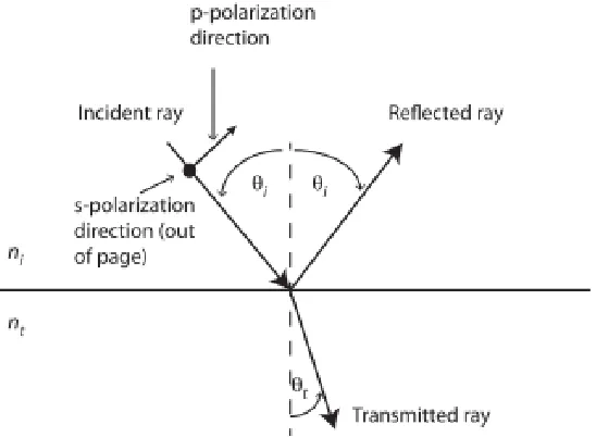
2.4 Specular reflection and refraction at an interface between two media [17]. . 25

2.5 Incident and reflected angles used in describing a surface’s bidirectional

scat-tering distribution function (BSDF) [17]. . . 27

2.6 Geometry for scattering from a source area to a collector area [67]. . . 28

(19)

xviii LIST OF FIGURES

2.7 Mircoscope image of surface roughness on a fused silica surface due to

grind-ing and polishgrind-ing. The image is approximately 10 µm across, with an RMS surface roughness of 5 ˚A [76]. . . 32

2.8 Vectors used in the Harvey-Shack scatter model [80]. . . 33

2.9 Example Harvey-Shack scatter model curve with L = 0.01, b0 = 0.1, and

S = −1.5. Assuming λ = 0.55 µm, these parameters correspond to an approximate surface roughness ofσRM S= 14.7 ˚A [81]. . . 35

2.10 Number of particles of diameter≥Dv. Daccording to IEST-STD-CC1246D for CLs 200, 400, and 600 [17]. . . 37

2.11 Example of how dendrites can be used to trap light. The angles of incidence

are defined according to the macroscopic surface normal and not the variable

dendrite profile. [17]. . . 39

2.12 Setup used for a veiling glare test [17]. . . 42

2.13 Stray light systems engineering flowchart illustrating the necessary steps from

stray light requirements definition to final system build and model

valida-tion [17]. . . 44

2.14 Strengths and weakness of the build-and-test v. model-and-predict methods

for stray light analysis [68]. . . 52

2.15 Image of a bar target (a) without stray light and (b) with stray light. Stray

light acts to reduce the contrast of the bar target. [17]. . . 59

2.16 DIRSIG simulation of the Port of Tacoma, WA imaged with a 2-D framing

(20)

LIST OF FIGURES xix

2.17 The 2-step PSF importance sampling process combines a single random pixel

location with a single random PSF offset: (a) One initial and final ray

sam-pling location. (b) Numerous initial and final ray samsam-pling locations. . . 77

2.18 DIRSIG image of a resolution test target and a helicopter with rotating rotor

blades: (a) No Gaussian PSF or time integration. (b) With a Gaussian PSF

and time integration. . . 78

3.1 Integrating optical engineering software programs with a radiative transfer

image simulation model combines the unique benefits of each type of sofware. 83

3.2 Integration method flowchart illustrating how system PSF and stray light

performance data collected from an optomechanical system model in optical

engineering software (blue steps) can be used to image a scene using a

ra-diative transfer image simulation model (orange steps) to produce simulated

output imagery. . . 83

3.3 As detailed by the integration method’s underlying radiometry, the stray light

contributions reaching the focal plane of an optical system are inherently a

product of the system’s stray light susceptibility and the scene’s at-aperture

radiance profile. . . 90

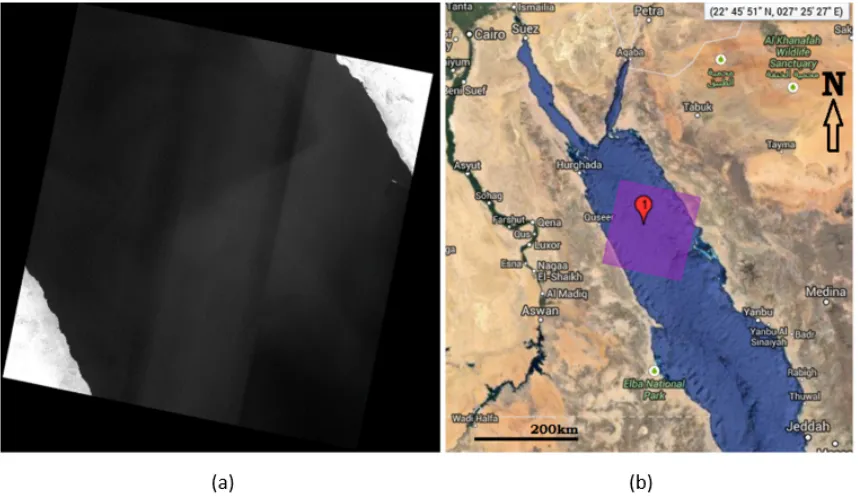
3.4 (a) TIRS band 11 (11.50–12.51 µm) image of the Red Sea with image inten-sity ranging from 8.5 to 11.5 W/m2/sr/µm. Far-field stray light leads to a banding effect that is evident in the across-track direction between the three

FPAs. (b) Map from USGS Earth Explorer showing the extent of the scene.

(21)

xx LIST OF FIGURES

3.5 Cassegrain telescope FRED model with a flat black paint scatter model (TIS

= 2% at normal incidence) assigned to the mechanical surfaces (labeled in

black). A Harvey-Shack scatter model (b0 = 0.1, L = 0.01, and S =−1.5) and Mie scatter model representing particulate contamination (CL400) have

been assigned to the optical surfaces (labeled in blue). . . 94

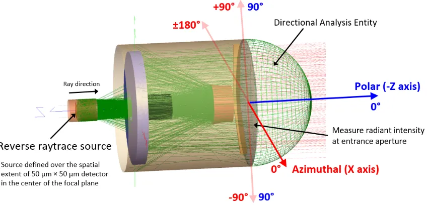
3.6 Reverse raytrace using the Cassegrain telescope model along with the stray

light ASM coordinate system. The system’s stray light susceptibility data is

captured at the entrance aperture as a radiant intensity profile by the DAE.

These data are then converted to stray light radiant flux per grid element by

multiplying by each DAE grid element’s solid angle. . . 96

3.7 Scatter model importance sampling demonstration. (a) Scatter rays into

the full hemisphere. (b) Scatter rays towards a detector. The latter case

produces greatly improved radiometric results due to the increased numbers

of rays scattered to the surface of interest [17]. . . 98

3.8 (a) Cassegrain system stray light ASM at 1° × 1° resolution (log of radiant

flux). (b) Visualization of the Cassegrain stray light ASM on the entrance

aperture DAE grid in FRED (log of radiant intensity). Azimuthal angle

(22)

LIST OF FIGURES xxi

3.9 Visualization of the Cassegrain telescope’s highest susceptibility stray light

path. In the forward direction, these rays enter the Cassegrain telescope’s

entrance aperture and scatter off of the primary mirror baffle’s inner wall

directly to the detector. In our reverse raytrace, this stray light path is

solely responsible for 46.9% of the total stray light radiant flux captured by

the detector’s stray light ASM. . . 102

3.10 Validation levels for end-to-end system modeling and simulation. Work

sup-porting the 2nd level of validation is presented in this dissertation, whereas

the 1st and 3rd levels have system and scene dependencies and are therefore

left to the users of this integration method. . . 108

4.1 Cassegrain telescope FRED model. The optical surfaces are labeled in blue

and the mechanical surfaces are labeled in black [60]. . . 116

4.2 Forward raytrace to capture the Cassegrain telescope’s on-axis PSF [60]. . . 117

4.3 Irradiance plot of the Cassegrain system on-axis PSF at λ = 0.55 µm (log scale). The black box denotes the spatial extent of a 9-µm FPA pixel [60]. . 117 4.4 System setup for the PSF validation tests. . . 119

4.5 Ideal result and DIRSIG output images for the 2-D RECT function PSF

validation test: (a) Ideal result. (b) 250 sampling rays per FPA pixel. (c)

500 sampling rays per FPA pixel. (d) 1,000 sampling rays per FPA pixel. (e)

10,000 sampling rays per FPA pixel. (f) 100,000 sampling rays per FPA pixel.128

4.6 Difference image between the ideal result and the DIRSIG image with 10,000

(23)

xxii LIST OF FIGURES

4.7 2-D correlation coefficient between the ideal result and the DIRSIG images

for each test case of the 2-D RECT function PSF validation test. The data

points indicate the mean value of the ten simulations conducted for each test

case, with the error bars extending plus or minus one standard deviation. . 130

4.8 RMSE in 2-D correlation coefficent v. number of DIRSIG sampling rays for

the 2-D RECT function PSF validation test. . . 131

4.9 Irradiance ratio for each test case of the 2-D RECT function PSF validation

test. The data points indicate the mean value of the ten simulations

con-ducted for each test case, with the error bars extending plus or minus one

standard deviation. . . 132

4.10 RMSE of the irradiance ratio v. number of DIRSIG sampling rays for the

2-D RECT function PSF validation test. . . 133

4.11 Ideal result and DIRSIG output images for the Cassegrain PSF validation

test (log scales): (a) FRED Cassegrain PSF. (b) 500 sampling rays per FPA

pixel. (c) 2,500 sampling rays per FPA pixel. (d) 10,000 sampling rays per

FPA pixel. (e) 25,000 sampling rays per FPA pixel. (f) 100,000 sampling

rays per FPA pixel. . . 135

4.12 2-D correlation coefficient between the FRED Cassegrain PSF and the DIRSIG

images for the Cassegrain PSF validation test. The data points indicate the

mean value of the ten simulations conducted for each test case, with the error

bars extending one standard deviation in each direction. . . 137

4.13 2-D correlation coefficent RMSE v. number of DIRSIG sampling rays for the

(24)

LIST OF FIGURES xxiii

4.14 Irradiance ratio for each test case of the Cassegrain PSF validation test. The

data points indicate the mean value of the ten simulations conducted for each

test case, with the error bars extending plus or minus one standard deviation. 140

4.15 RMSE of the irradiance ratio v. number of DIRSIG sampling rays for the

Cassegrain PSF validation test. . . 141

5.1 Simple FRED setup of two parallel aligned square surfaces for use in the

first stray light validation test. A source placed directly above the source

area illuminates the Lambertian source surface, scattering rays towards the

collector. The scatter radiant flux captured by the collector during a series

of FRED raytraces can then be compared to the analytically calculated value. 150

5.2 Integration method stray light radiant flux contribution equation in graphical

form: (top) Cassegrain stray light ASM converted to radiant flux. (middle)

0.10° circle target source ERM from DIRSIG integrated over the detector’s

spectral bandpass. (bottom) Stray light radiant flux contribution map. The

summation of the stray light radiant flux contribution map provides the

de-tector’s total stray light radiant flux. . . 167

6.1 Different scatter models applied to the Cassegrain telescope’s optical and

mechanical surfaces to represent various stray light performance conditions. 174

6.2 DIRSIG “LA scene” covering 450×375 km of central and southern California.177 6.3 Wide-area view of the DIRSIG LA scene with lower-resolution Earth

back-ground and inset outlining the LA scene location. . . 178

6.4 DIRSIG LA scene with Santa Barbara scene location within the Cassegrain

(25)

xxiv LIST OF FIGURES

6.5 LA scene with Earth background for the different combinations of DIRSIG

scene conditions (common log scales of spectral radiance at λ = 0.55µm). The very small black box near the center of each scene marks the Cassegrain

telescope’s nominal FOV over Santa Barbara, CA. (a) 1 Aug 2019 at 1:15

p.m. PDT with wind speed = 2.5 m/s W to E. (b) 1 Aug 2019 at 1:15 p.m.

PDT with wind speed = 7.5 m/s W to E. (c) 1 Aug 2019 at 11:30 a.m. PDT

with wind speed = 7.5 m/s W to E. (d) 1 Apr 2019 at 1:15 p.m. PDT with

wind speed = 7.5 m/s W to E. . . 182

6.6 Face-on view of the Cassegrain FPA detailing the pixel numbering scheme

used in FRED for capturing the shift-variant stray light ASMs. This is

necessary to keep track of which stray light ASM was collected for each FPA

pixel. . . 185

6.7 Block diagram of the integration method’s stray light radiant flux

contribu-tion equacontribu-tion. The ERM of a scene is multiplied solid angle grid

element-by-solid angle grid element with a detector element’s stray light ASM for a

given set of system stray light susceptibility conditions to produce the

de-tector element’s stray light radiant flux contribution map. The summation

of the stray light radiant flux contributions for each solid angle grid element

across the contribution map provides the detector element’s total stray light

(26)

LIST OF FIGURES xxv

6.8 Nominal irradiance images for Harvey-Shack mirror surface roughness (σRM S =

14.7 ˚A) and CL400 particulate contamination (common irradiance scale). (a) 1 Aug 2019 at 1:15 p.m. PDT with wind speed = 2.5 m/s. (b) 1 Aug 2019

at 1:15 p.m. PDT with wind speed = 7.5 m/s. (c) 1 Aug 2019 at 11:30 a.m.

PDT with wind speed = 7.5 m/s. (d) 1 Apr 2019 at 1:15 p.m. with wind

speed = 7.5 m/s. . . 192

6.9 Cassegrain telescope stray light ASMs for a pixel near the center of the

FPA (x356 y356) with system stray light susceptibility conditions including

Harvey-Shack mirror surface roughness (σRM S = 14.7 ˚A), CL400 particulate

contamination, and flat black paint TIS = 2% (common log of radiant flux

scale). (a) 10 million initial rays. (b) 100 million initial rays. The greater

number of rays traced in the latter case has reduced the statistical noise of

the system stray light susceptibility data. . . 194

6.10 Cassegrain telescope stray light ASMs for a pixel in the center of the FPA

(x356 y356) with varying system stray light susceptibility conditions:

(com-mon log of radiant flux scale). All of the system conditions have Harvey-Shack

mirror surface roughness (σRM S = 14.7 ˚A) included. (a) CL400 particulate

contamination and flat black paint TIS = 2%. (b) CL400 particulate

contam-ination and flat black paint TIS = 1%. (c) CL600 particulate contamcontam-ination

(27)

xxvi LIST OF FIGURES

6.11 Cassegrain telescope shift-variant stray light ASMs for various pixels across

the FPA (common log of radiant flux scale). The system stray light

suscep-tibility conditions include Harvey-Shack mirror surface roughness (σRM S =

14.7 ˚A), CL400 particulate contamination, and flat black paint TIS = 2%. All FPA pixel locations are based on viewing the FPA face on in the FRED

model (y-axis pointing up, x-axis pointing to the left). (a) top left corner

(pixel x5 y5). (b) top right (pixel x716 y5). (c) center (pixel x356 y356). (d)

bottom left (pixel x5 y716). (e) bottom right (pixel x716 y716). . . 200

6.12 DIRSIG ERMs for the different scene conditions (common log of spectral

radiance scale). The black circles at the top center of each plot marks the

Santa Barbara scene location for reference. (a) 1 Aug 2019 at 1:15 p.m. PDT

with wind speed = 2.5 m/s. (b) 1 Aug 2019 at 1:15 p.m. PDT with wind

speed = 7.5 m/s. (c) 1 Aug 2019 at 11:30 a.m. PDT with wind speed = 7.5

(28)

LIST OF FIGURES xxvii

6.13 Illustration of how the azimuthal angles where different FPA pixels have

their highest stray light susceptibility map to the scene. The scene shown

is 1 Aug 2019 at 1:15 p.m. with wind speed = 2.5 m/s plotted on a linear

spectral radiance scale. (a) The orange arrows mark the azimuthal angle of

highest susceptibility for the labeled FPA corner pixels. The red arrows map

the Cassegrain telescope’s stray light ASM azimuthal angles to the scene

(polar angle θ= 0° points directly into the page). The very small black box in the center of the scene outlines the Cassegrain telescope’s nominal FOV

over Santa Barbara, CA. (b) Face-on view of the Cassegrain FPA within

the FRED model with the corner pixel locations labeled and scene cardinal

directions mapped to the FPA. . . 204

6.14 Orientation of the Cassegrain FPA within the FRED model to the DIRSIG

FPA used to produce the nominal, stray light, and combined final output

images. The Cassegrain FPA must be flipped vertically to match the DIRSIG

FPA. As detailed by the cardinal directions, this specific orientation of the

DIRSIG FPA was chosen so that north in the Santa Barbara scene points up,

(29)

xxviii LIST OF FIGURES

6.15 Stray light irradiance images for the 1 Aug 2019 at 1:15 p.m. PDT, wind

speed = 2.5 m/s scene with different system stray light susceptibility

con-ditions. Note that every image has a different irradiance scaling to best

highlight its unique distribution. All system stray light susceptibility

condi-tions include Harvey-Shack mirror surface roughness (σRM S = 14.7 ˚A). (a)

Large-area view of the scene for 1 Aug 2019 at 1:15 p.m. PDT with wind

speed = 2.5 m/s for reference. The small black box in the center of the scene

outlines the Cassegrain telescope’s FOV. (b) No particulate contamination,

flat black paint TIS = 2%. (c) CL400, flat black paint TIS = 1%. (d) CL400,

flat black paint TIS = 2%. (e) CL600, flat black paint TIS = 1%. (f) CL600,

flat black paint TIS = 2%. . . 207

6.16 Stray light irradiance images for the stray light susceptibility conditions with

Harvey-Shack mirror surface roughness (σRM S = 14.7 ˚A), CL400 particulate

contamination, and flat black paint TIS = 2% for each of the different scene

conditions. Note that every image has a different irradiance scaling to best

highlight its unique distribution. (a) 1 Aug 2019 at 1:15 p.m. PDT, wind

speed = 2.5 m/s. (b) 1 Aug 2019 at 1:15 p.m. PDT, wind speed = 7.5 m/s.

(c) 1 Aug 2019 at 11:30 a.m. PDT, wind speed = 7.5 m/s. (d) 1 Apr 2019

(30)

LIST OF FIGURES xxix

6.17 Stray light radiant flux contribution maps for the 1 Aug 2019 at 1:15 p.m.

PDT, wind speed = 2.5 m/s scene and system stray light susceptibility

condi-tions with Harvey-Shack mirror surface roughness (σRM S = 14.7 ˚A), CL400

particulate contamination, and flat black paint TIS = 2% (common log of

radiant flux scales). The summation of these stray light radiant flux

con-tribution maps provides the total stray light radiant flux for the given FPA

pixel. (a) Pixel x5 y5 (bottom left of DIRSIG Cassegrain FPA) (b) Pixel

x716 y716 (top right of DIRSIG Cassegrain FPA). . . 212

6.18 The nominal (top left) and stray light (top right) images for a given set

of system stray light susceptibility and scene conditions are added together

to form the final output image (bottom center). This example is for the 1

Aug 2019 at 1:15 p.m. PDT, wind speed = 2.5 m/s scene and system stray

light susceptibility conditions with Harvey-Shack mirror surface roughness

(σRM S = 14.7 ˚A), CL400 particulate contamination, and flat black paint

TIS = 2%. Note that the nominal and final output images are plotted on the

same irradiance scale. . . 216

6.19 Percent stray light images for the 1 Aug 2019 at 1:15 p.m. PDT, wind speed

= 2.5 m/s scene with different system stray light susceptibility conditions

(common percent stray light scaling). All system stray light susceptibility

conditions include Harvey-Shack mirror surface roughness (σRM S = 14.7 ˚A).

(a) No particulate contamination, flat black paint TIS = 2%. (b) CL400, flat

black paint TIS = 1%. (c) CL400, flat black paint TIS = 2%. (d) CL600,

(31)

xxx LIST OF FIGURES

6.20 Percent stray light images for the system stray light susceptibility conditions

with Harvey-Shack mirror surface roughness (σRM S = 14.7 ˚A), CL400

par-ticulate contamination, and flat black paint TIS = 1% across the different

scene conditions. Note that every image has a different irradiance scaling to

best highlight its unique distribution. (a) 1 Aug 2019 at 1:15 p.m. PDT,

wind speed = 2.5 m/s. (b) 1 Aug 2019 at 1:15 p.m. PDT, wind speed = 7.5

m/s. (c) 1 Aug 2019 at 11:30 a.m. PDT, wind speed = 7.5 m/s. (d) 1 Apr

2019 at 1:15 p.m. PDT, wind speed = 7.5 m/s. . . 222

6.21 Ideal Cassegrain telescope final output image and the final output images

(nominal + stray light image) of 1 Aug 2019 at 1:15 p.m. PDT, wind speed

= 2.5 m/s scene under different stray light susceptibility conditions

(com-mon irradiance scale). All system stray light susceptibility conditions include

Harvey-Shack mirror surface roughness (σ= 14.7 ˚A). Note that every image has the same irradiance scaling to best highlight the contrast reduction

com-pared to the ideal image. (a) Ideal Cassegrain system. (b) No particulates,

BP TIS = 2%. (c) CL400, BP TIS = 1%. (d) CL400, BP TIS = 2%. (e)

(32)

List of Tables

3.1 Cassegrain telescope designed optical path in the forward direction (object

space to focal plane). . . 95

3.2 Percentage of the total stray light radiant flux on the detector’s stray light

ASM from first-order stray light paths including significant scattering

sur-faces. The surfaces listed are where the single scattering event took place in

each case. Since many unique first-order stray light paths can share the same

scatter surface, these percentages are the summation of all first-order stray

light paths for each scatter surface. . . 102

4.1 Number of DIRSIG sampling rays per FPA pixel tested for the PSF validation

tests. . . 124

(33)

xxxii LIST OF TABLES

5.1 Comparison between the collector scatter radiant flux analytical calculation

and the FRED raytrace results for the source-collector test setup. The FRED

raytrace results display the mean and standard deviation of the collector

scatter radiant flux across the twenty raytraces conducted. The difference

from analytical indicates the percentage difference between the mean raytrace

collector scatter radiant flux and the analytically calculated value. . . 160

5.2 Comparison between the detector scatter radiant flux for the original

ana-lytical calcluation, FRED forward raytraces, and FRED reverse raytraces.

The FRED raytrace results display the mean and standard deviation of the

detector scatter radiant flux across the twenty raytraces conducted in each

case. . . 162

5.3 Comparison of the mirror GCFs in the original Peterson analytical equation

and the corrected GCFs from FRED for the detector as seen by each mirror. 163

5.4 Comparison of the system transmittances at each mirror used in the

orig-inal Peterson analytical equation and the corrected system transmittances

from FRED taking into account projection effects from the target source and

mechanical components. . . 163

5.5 Comparison between the detector scatter radiant flux for the original and

corrected analytical calcluations and the FRED forward raytrace. The FRED

raytrace results display the mean and standard deviation of the detector

(34)

LIST OF TABLES xxxiii

5.6 Comparison between the FRED forward and reverse raytrace results and

the integration method applied to the simplified Cassegrain telescope and

circular target source imaging scenario. Each set of results display the mean

and standard deviation of the detector scatter radiant flux across the twenty

raytraces conducted in each case. . . 168

6.1 Different combinations of stray light performance conditions. All cases

in-clude the same Harvey-Shack scatter model (b0 = 0.1, L = 0.01, and S =

−1.5; σRM S = 14.7 ˚A) for optical surface roughness. The flat black paint

TIS percentages refer to the value at normal incidence. . . 175

6.2 Different combinations of DIRSIG scene conditions. All times of day are

listed in Pacific Daylight Time (PDT). . . 181

6.3 The Cassegrain telescope G#’s for different optical surface conditions. Note

that these G#’s are all calculated for the center of the focal plane. The

Harvey-Shack scatter model includes b0 = 0.1, L = 0.01, and S = −1.5, which corresponds to σRM S = 14.7 ˚A atλ= 0.55µm. . . 191

6.4 Total stray light (SL) radiant flux and pixel percent stray light for a pixel

(x356 y356) near the center of the Cassegrain telescope’s FPA under different

system stray light susceptibility conditions. “BP” refers to the flat black paint

scatter model assigned to the mechanical components and the TIS values are

for normal incidence. All of the system conditions include Harvey-Shack

(35)

xxxiv LIST OF TABLES

6.5 Mean irradiance values for the stray light images of the 1 Aug 2019 at 1:15

p.m. PDT, wind speed = 2.5 m/s scene with different system stray light

susceptibility conditions. . . 208

6.6 Mean of the irradiance values for the stray light images with Harvey-Shack

mirror surface roughness (σRM S = 14.7 ˚A), CL400 particulate contamination,

and flat black paint TIS = 2% for each of the different scene conditions. . . 211

6.7 Percentage of the total stray light irradiance for pixel x5 y5 that originates

from sources within the given polar angle ranges in object space. These data

are for the 1 Aug 2019 at 1:15 p.m. PDT, wind speed = 2.5 m/s scene

and system stray light susceptibility conditions with Harvey-Shack mirror

surface roughness (σRM S = 14.7 ˚A), CL400 particulate contamination, and

flat black paint TIS = 2%. The components causing scatter are the major

scatter contributors for each polar angle range. . . 214

6.8 Percentage of the total stray light irradiance for pixel x716 y716 that

origi-nates from sources within the given polar angle ranges in object space. These

data are for the 1 Aug 2019 at 1:15 p.m. PDT, wind speed = 2.5 m/s scene

and system stray light susceptibility conditions with Harvey-Shack mirror

surface roughness (σRM S = 14.7 ˚A), CL400 particulate contamination, and

flat black paint TIS = 2%. The components causing scatter are the major

scatter contributors for each polar angle range. . . 214

6.9 Mean percent stray light values for the land and water pixels across all

(36)

LIST OF TABLES xxxv

6.10 Contrast values and reductions from the ideal images to final output images

(nominal + stray light images) across every combination of system stray light

susceptibility and scene conditions. All of the system stray light susceptibility

(37)

(38)

Chapter 1

Introduction

1.1

CONTEXT

Since its very formation, the Earth has been a dynamic world of change. Natural forces

have dramatically altered the landscape, with rivers and glaciers slowly etching away valleys

and canyons, tectonic plates colliding to form towering mountain ranges and triggering

jarring earthquakes, volcanoes spewing forth lava to create new land, and both wind and

precipitation eroding and weathering the surface. Biological forces have also played a role,

as animals and plants combine to form complex and diverse ecosystems that evolve over

time. We as humans have altered the Earth in dramatic ways by building sprawling cities,

planting fields of crops, cutting down forests, diverting water resources to barren lands, and

polluting the environment.

Collecting data to monitor and analyze these global changes has been an arduous manual

task for much of human history. As transportation and communication evolved, more

information could be gathered and shared about our ever-changing world. The dawn of

(39)

2 CHAPTER 1. INTRODUCTION

flight greatly improved our ability to capture global change information via remote sensing,

the acquisition of information about objects or phenomena without coming into physical

contact with the target. Medium-to-high resolution Earth imagery from low-flying aircraft

could be collected and pieced together to produce aerial views that no human had ever

seen before. However, it was the advent of satellites that truly revolutionized our capability

to collect detailed information about the entire Earth. Satellites present many advantages

for remote sensing, including synoptic views (“big-picture” views of large areas), periodic

revisits of specific ground locations, and the ability to collect data quickly, over inaccessible

areas, and simultaneously at different wavelengths and modalities using a single platform.

Although much of the nascent United States space program focused on manned missions,

the concept of an Earth-orbiting satellite to monitor natural resources was first advocated by

the Department of the Interior and the U.S. Geological Survey (USGS) in the early 1960s [1].

On July 23, 1972, the National Aeronautics and Space Administration (NASA) launched the

Earth Resources Technology Satellite (ERTS), the first satellite with the expressed intent

to study and monitor the Earth’s landmasses [2]. Once a duplicate ERTS was launched in

1975, the two satellites were renamed Landsat 1 and Landsat 2. A total of seven successful

Landsat missions have collected some six million multispectral images of the Earth over

the past forty-seven years, establishing Landsat as the longest running, space-based Earth

observation program [3]. Figure 1.1 shows the operational lifetime for each mission, clearly

detailing the fact that at least one Landsat satellite has been active at any given time

since the program’s first launch. Although instrument advancements have led to better

radiometry, improved spatial resolution, and the addition of new spectral bands over the

course of the Landsat program’s lifetime, its core visible and near-infrared (NIR) spectral

(40)

1.1. CONTEXT 3

temporal record of the Earth that has made Landsat so essential for conducting global

change research; maintaining and extending this historical record into the future remains

a key priority of the program. Although only a brief overview of the Landsat program’s

history is provided here, more extensive historical details and the characteristics of specific

missions have been chronicled elsewhere [1, 4–6].

Figure 1.1: Landsat program timeline with the operational on-orbit duration of each mis-sion [7].

The world has undergone significant change over the Landsat program’s roughly

half-century lifetime, particularly from the growth of the world population and economy. There

are numerous scientific, economic, and humanitarian applications that benefit from

Land-sat’s imagery documenting these global changes, including agriculture, forestry, geology,

re-gional planning, disaster relief, natural resource monitoring, climate research, and land use

and cover analysis [8–10]. Although there are increasing numbers of international and

com-mercial moderate-resolution Earth-orbiting satellites, Landsat remains the so-called “gold

standard” of land remote sensing for its unique ability to meet the following five criteria [1]:

(41)

4 CHAPTER 1. INTRODUCTION

change, yet sufficiently coarse to allow for seasonal coverage of the globe.

2. Landsat provides spectral coverage in the visible and NIR, with additional bands in

the short-wave infrared (SWIR) and thermal-infrared regions.

3. Landsat data is calibrated to science-quality at-sensor radiance and reflectance, so

long-term changes in the land can be separated from varying trends in instrument

performance.

4. Landsat collects data from all over the globe, providing seasonal coverage of all land

masses.

5. Landsat data is freely available and open to distribution.

Landsat 8, the most recent addition to the program, launched in February 2013; Landsat

9, a successor satellite, is currently under development and slated for a tentative launch

date in December 2020 [11]. In an effort to maintain the almost half-century record of

data continuity, NASA and the USGS have already initiated technology and requirement

studies for a future Landsat 10 to launch later in the 2020s [12]. Whereas Landsat 9 will

largely replicate its Landsat 8 predecessor, NASA and the USGS are investigating

long-term mission architectures and technological innovations that will enhance the imaging

capabilities of Landsat 10 and beyond [12].

Some of the Landsat 10 mission architecture options include launching constellations of

satellites with more compact, lower cost designs, which could provide improved temporal

coverage of the Earth, a priority for future Landsat systems [12]. Throughout the Landsat

program’s history, advancements in focal plane array (FPA) technology have led to an

(42)

1.1. CONTEXT 5

and enabling overall system miniaturization and reduced cost [13]. In recent years, the

emergence of freeform optical components, which contain optical surfaces that have no

rotational symmetry about any axis, has vastly expanded the toolbox of optical designers.

Freeform optics allow for improved image quality and reduced aberrations while using fewer

overall optical components that are reduced in size, thus offering the potential for cost

savings [14–16]. Despite the mission benefits, compact instrument designs also increase the

number of overlapping optical paths and reduce opportunities for controlling stray light,

such as inserting baffles.

In a simplistic sense, stray light is defined as any unwanted radiation that reaches the

focal plane of an optical system. Stray light occurs because it is not possible to perfectly

control every ray of light that enters a system and direct it to the proper location on the

focal plane [17]. Stray light can be created by a number of mechanisms, including surface

roughness due to material properties or as a result of manufacturing techniques, ghost

reflections from light rays that reflect off of lens surfaces, diffraction from apertures,

self-emission of optical components in thermal systems, or atmospheric scattering. Control of

this unwanted stray light is important in scenarios where one is observing faint objects near

bright sources, when high radiometric precision or contrast is required, when imaging with

infrared camera systems susceptible to thermal self-emission, or when making multispectral

or hyperspectral measurements that can result in spectral crosstalk [17]. Stray light is a

particular concern for the Landsat program and its myriad scientific applications, which

rely upon radiometrically calibrated data [18]. Stray light acts as a form of optical noise

that obscures the desired signal, degrading scientific accuracy and potentially preventing

meaningful analysis altogether [19].

(43)

6 CHAPTER 1. INTRODUCTION

unique to the Landsat program. The U.S. Department of Defense (DoD) has conducted

studies on the resiliency benefits of satellite disaggregation, distributing the capabilities of

larger satellites into multiple smaller spacecraft, to preserve the United States’ operational

advantage in space [20,21]. The past decade has also witnessed the proliferation of cubesats

and nanosats, as space agencies, militaries, universities, and commercial companies across

the world are interested in small satellites for a wide range of applications. The design

constraints inherent in these compact systems lead to tighter systems engineering

trade-offs, underscoring the need to better understand the quantitative linkage between stray

light performance and impact to user applications.

Current stray light research is largely deficient in clearly relating system stray light

requirements and performance to user application impact. Much of the stray light literature

analyzes the pre-mission stray light performance of a specific optomechanical system [18,

22–28], provides an assessment of how well a system’s operational stray light performance

matches its predicted performance [29–31], or introduces post-processing methods to correct

for stray light in imagery [30,32–37]. The pre-mission and operational assessments generally

focus on stray light requirement verification rather than validating that a system’s stray

light performance is acceptable for user applications. This indicates an implicit trust that

a system’s stray light requirements have been properly defined, i.e. that the system will

satisfy user expectations if its stray light performance meets the requirements.

However, stray light performance depends on many different optomechanical design

parameters, thus complicating the task of drafting suitable stray light requirements for a

specific system and its range of user applications. As a result, stray light requirements are

often based on historical requirements from similar previous missions rather than explicitly

(44)

1.1. CONTEXT 7

manner runs the risk of overestimating the level of stray light performance truly needed for

a system, leading to additional costs and delays building in the performance margin. At

worst, the new system’s design or user applications may be inherently more susceptible to

stray light and the heritage-derived requirements will not be sufficient, resulting in possible

redesign of the entire system or risking a dissatisfied user community. In fact, in the

worst case scenario, it may not even be possible for the new system to meet more strict

heritage-derived stray light requirements while meeting all other system requirements. The

practice of simply using more stringent heritage-derived stray light requirements and over

engineering a system’s stray light performance with sufficient margin is less feasible in the

future as systems push theoretical and manufacturing limits (e.g. compact systems using

freeform optics) [38]. It is evident that a method is needed to set stray light requirements

based upon a clear quantitative linkage to the acceptable levels of stray light for user

applications.

Beyond the challenge of stray light requirement definition and justification, a significant

amount of stray light-related research focuses on characterizing a system’s point spread

function (PSF) through direct measurement [39–41], image analysis [1, 42–47], or

mathe-matical modeling [36, 46, 48–52]. The characterization of a system’s stray light performance

through PSFs is intrinsically limited to near-field stray light, which originates from sources

in or near a detector element’s instantaneous field of view (IFOV), while ignoring far-field

stray light originating from sources farther beyond the IFOV. Focusing on near-field stray

light therefore almost entirely excludes stray light from sources outside of a system’s field

of view (FOV), which can scatter off mechanical components or optical component surface

roughness and particulate contamination or undergo ghost reflections, thus resulting in

(45)

8 CHAPTER 1. INTRODUCTION

presented that include out-of-FOV stray light sources for astronomical applications [53–56],

but these have been applied to more restricted operational scenarios and scenes of

inter-est. Other methods have used out-of-FOV stray light source mapping in conjunction with

empirical weightings for post-processing stray light correction [57, 58].

The need remains to incorporate a system’s comprehensive susceptibility to stray light

(i.e. near-field and far-field) in a predictive assessment of its Earth-observing performance

imaging a scene of interest under a range of operational scenarios. With a sufficient solution,

system trade studies and sensitivity analyses could then be conducted to quantitatively link

detailed design parameters influencing an Earth-observing system’s stray light performance

to their impact on user applications. This problem is not only limited to stray light, as there

is a general systems engineering need to analyze the impact of specific optomechanical design

parameters on user applications and to draft informed system requirements that minimize

negative impact while optimizing cost.

In summary, the current state of stray light analysis for imaging systems is deficient in

the following respects:

Existing stray light analyses focus more on stray light requirement verification rather

than validating that stray light levels meet user application needs.

Existing stray light requirements lack sufficient quantitative justification traceable to

user applications.

Existing modeling and simulation techniques are inadequate to conduct end-to-end

stray light-focused system trade studies or sensitivity analyses that quantitatively

link system design parameters or decisions to user application impact when imaging

(46)

1.1. CONTEXT 9

From these deficiencies, it is apparent that an end-to-end stray light modeling and

simula-tion capability is needed, where optomechanical design trade studies can be explored using

system software models and the resulting user application impact of each system condition

assessed on realistic operational scenes. This capability would lead to more informed

sys-tem design decisions and the writing of stray light and syssys-tem requirements with a direct

understanding of user impact. Additionally, this capability would aid in testing stray light

correction algorithms pre-mission, so that decisions could be made to either change the

system design for improved stray light performance or to correct for the observed levels of

stray light via post-processing.

The Digital Imaging and Remote Sensing (DIRS) Laboratory at the Rochester Institute

of Technology (RIT) has a decades-long history of partnering with NASA and the USGS

in researching technical areas of interest for the Landsat program. To address the needs

presented here, we have developed a novel modeling and simulation-based methodology to

integrate optomechanical system software models with a radiative transfer image simulation

model that incorporates the rest of the imaging chain [59]. This capability enables users to

assess the PSF and stray light performance of optomechanical system software models on

high-fidelity simulations imitating realistic operational scenes [60]. The methodology first

characterizes a system’s PSF and stray light susceptibility through the collection of raytrace

data from a 3-D computer-aided design (CAD) optomechanical system model using optical

engineering software. This process is greatly enhanced by using optical engineering

soft-ware’s new graphical processing unit (GPU) raytracing capabilities. These raytrace data

are then integrated with a radiative transfer image simulation model to simulate the

imag-ing of a complex, highly-realistic scene description and evaluate the system’s operational

(47)

10 CHAPTER 1. INTRODUCTION

software integration.

Figure 1.2: Integrating an optomechanical system model from optical engineering software with a radiative transfer image simulation model combines the unique benefits of each type of model in creating the complete imaging chain.

In the work presented here, we use FRED Optical Engineering Software [61] by

Pho-ton Engineering and the Digital Imaging and Remote Sensing Image Generation (DIRSIG)

model [62], a physics-based scene creation and image and data simulation model

devel-oped at RIT, to validate and demonstrate the software integration method. However, our

integration method generalizesto any optical engineering software program capable of

col-lecting the necessary PSF and stray light raytrace data andto any radiative transfer image

simulation model that can create physics-based scenes and incorporate the captured PSF

and stray light performance data. Although stray light is the impetus for this research,

the integration methodology is versatile and can be used to investigate other parameters

of interest, including image quality, the effects of aberrations and distortions, tolerancing

and alignment of optical and mechanical components, or degradation expected during a

(48)

1.2. OBJECTIVES 11

1.2

OBJECTIVES

We have defined a set of research objectives to address the needs and shortcomings of current

stray light analysis, modeling and simulation capabilities, and requirement definition.

Objective 1: Demonstrate a general methodology for integrating optomechanical

sys-tem software models with a radiative transfer image simulation model.

Objective 2: Validate the integration method’s capability to accurately incorporate

point spread function (PSF) performance data from an optomechanical system

soft-ware model.

Objective 3: Validate the integration method’s capability to accurately incorporate

stray light performance data from an optomechanical system software model.

Objective 4: Demonstrate the integration method’s system trade study capability

using various system stray light susceptibility and scene conditions.

Objective 5: Demonstrate how the integration method can be used to produce

quan-titative metrics that are useful in determining the impact of stray light on user

appli-cations.

1.3

DISSERTATION LAYOUT

1.3.1 Chapter 2: Background

This chapter provides an introduction to stray light, including its fundamental mechanisms,

causes, and metrics, as well as the primary methods to analyze system stray light

(49)

12 CHAPTER 1. INTRODUCTION

analysis within the system design process is emphasized and the capabilities of modern

optical engineering software programs are reviewed. An overview of linear systems theory

is provided to introduce necessary details regarding system imaging performance. Finally,

previous efforts to model and simulate imaging system performance are discussed, focusing

on those modeling stray light or using DIRSIG.

1.3.2 Chapter 3: Integration Methodology (Objective 1)

This chapter provides an overview of the integration method’s basic radiometric framework,

including a mathematical explanation of the PSF and stray light components. These two

components are then discussed in terms of the specific data that must be collected from

an optomechanical system software model to incorporate their contributions into the

in-tegration method. The collection and analysis of stray light performance data from an

optomechanical system software model is demonstrated in order to better illustrate this key

component of the integration method.

1.3.3 Chapter 4: Point Spread Function Component Validation (Objec-tives 1 & 2)

This chapter covers the details of the integration method’s PSF component, including how

PSF data can be collected from an optomechanical system software model. Two tests are

presented to validate a method for using PSF data to image a scene within a radiative

transfer image simulation model and to validate the successful incorporation of PSF data

from an optomechanical system software model with a radiative transfer image simulation

(50)

1.4. NOVEL CONTRIBUTIONS 13

1.3.4 Chapter 5: Stray Light Component Validation (Objectives 1 & 3)

This chapter includes several tests to validate the stray light radiometry of an optical

engineering software program and the integration method itself. This provides confidence

to users of the integration method that the stray light component can produce accurate

stray light radiometry for an arbitrary system and scene.

1.3.5 Chapter 6: System Trade Study Demonstration (Objectives 1, 4, & 5)

This chapter presents an in-depth demonstration of the integration method’s capability to

perform a stray light-focused system trade study. This case study is performed using a

Cassegrain telescope model and a coastal scene of southern California. Quantitative stray

light metrics are presented and discussed in detail to provide insights into the application

of the integration method for an arbitrary system and scene.

1.3.6 Chapter 7: Summary and Conclusions

This chapter summarizes the research motivation and objectives, the work that has been

performed and its innovative contributions, presents final conclusions, and recommends

future work.

1.4

NOVEL CONTRIBUTIONS

The novel contributions of this research include the following items:

Development and validation of a general methodology for the integration of

(51)

14 CHAPTER 1. INTRODUCTION

Validation of an importance sampling-based approach for emulating PSF convolution

in-the-loop of a simulation performed using a radiative transfer image simulation

model.

Development and validation of a method to estimate the stray light irradiance of each

detector element across the focal plane given an optomechanical imaging system’s

shift-variant stray light susceptibility and a scene’s at-aperture radiance profile.

Demonstration of optical engineering software’s GPU raytracing capability to

col-lect detailed shift-variant system stray light susceptibility data for use in conducting

system trade studies.

Introduction of simulated stray light irradiance images that include stray light

contri-butions from all of object space for any combination of system stray light susceptibility

and scene conditions.

Introduction of detailed performance data that take into account both a system’s stray

light susceptibility and a scene’s at-aperture radiance profile to determine the stray

light contribution of specific components, ray paths, or scene elements.

Demonstration of the integration method’s capability to perform stray light-focused

system trade studies using stray light-stressing remote sensing scenes in order to

(52)

Chapter 2

Background

This chapter is provided as a more in-depth examination of the fundamentals of stray light,

linear systems theory, and the modeling and simulation of imaging systems.

2.1

RADIOMETRIC TERMS

It is important to define a few radiometric terms before delving into the discussion on

stray light. The definitions presented here are consistent with internationally recognized

standards [63], and these terms will be used throughout the background discussion and

subsequent chapters. International System of Units (SI) measurements are listed in brackets

[ ] for these quantities.

(53)

16 CHAPTER 2. BACKGROUND

2.1.1 Radiant Energy

The energy of a single photon of light,q, is given by

q=hν= hc

λ [joules,J], (2.1)

whereh≈6.626×10−34J·s is Planck’s constant,νis the photon’s frequency,c≈2.998×108 m/s is the speed of light, andλis the photon’s wavelength [m]. It is apparent from Eq. 2.1 that shorter wavelength photons carry more energy than lower wavelength photons.

The total energy,Q, of a beam of light is a summation of the number of photons at each wavelength, calculated according to

Q=Xqi =

X

i

nihν=

X

i

nihc

λi

[J], (2.2)

whereni is the number of photons at each wavelength,λi.

2.1.2 Radiant Flux

It is often more useful to consider the rate at which energy impinges on a surface rather

than the total energy deposited. The radiant flux, or power (Φ), is the energy flow to or

from a surface and is the first derivative of the radiant energy with respect to time (t), i.e.,

Φ = dQ

(54)

2.1. RADIOMETRIC TERMS 17

2.1.3 Irradiance

In imaging systems, we are typically interested in the amount of radiant flux that is received

by a certain area (e.g. a detector). This quantity is named irradiance (E) and is defined as

E = dΦ

dA [W· m

−2_]_. _(2.4)

Although Eq. 2.4 is written as a differential quantity, it is important to note that irradiance

can vary across a surface and therefore has an implicit spatial dependence, i.e. E(x, y). The total radiant flux on a surface can be calculated by integrating the irradiance distribution

over the surface area according to

Φ =

Z

Area

E(x, y) dA [W]. (2.5)

If a source is not pointing directly nadir, but is tilted by an angle, θ, relative to the receiving object, then the projected area of the object must be used instead. This introduces

a cosθ factor, as given by

Eθ =E0cosθ [W· m−2]. (2.6)

where Eθ is the irradiance on the projected surface and E0 is the irradiance if the source were perpendicular to the surface. The irradiance over the projected area will necessarily

be reduced, since the same incident radiant flux is spread over a larger area.

2.1.4 Radiant Intensity

Although irradiance details the amount of radiant flux per unit area, it provides no angular

(55)

18 CHAPTER 2. BACKGROUND

of radiant flux with no spatial description. The angular dependence is described in terms of

solid angle, which has units of steradians (sr), and is given by dΩ = dA/r2[m_m22 = sr], where

dA can be thought of as the differential area projected onto a spherical surface of radiusr. Radiant intensity is therefore defined as

I = dΦ

dΩ [W· sr

−1_]_. _(2.7)

2.1.5 Radiance

Radiance is a more complex quantity than those previously described, combining the spatial

and angular dependencies of radiant flux into one term. Radiance is the flux per unit area

per unit solid angle and is given by

L=L(x, y, θ, φ) = d 2_Φ

cosθdAcosσdΩ [W·m

−2_· _sr−1_]_, _(2.8)

where θ and φ are the polar and azimuthal angles relative to the normal to the plane, respectively, and the cosθ and cosσ factors are included to account for area projection effects of both the source and collector, respectively. Radiance is often used in radiometry

due to its invariance over distance, assuming no transmission losses.

The radiant flux of a source with radiance Lis calculated by integrating over both area and solid angle, i.e.

Φ =

Z

A

Z

Ω

L(x, y, θ, φ) cosθdAcosσdΩ [W]. (2.9)

As with all of the other quantities defined in this section, radiance can have a spectral

(56)

2.2. STRAY LIGHT 19

evaluated at a specific wavelength is given by

Lλ=

dL(x, y, θ, φ)

dλ =

d3Φ

cosθdAcosσdΩ dλ [W·m

−2_· _sr−1_· _µ_m−1_]_. _(2.10) Here we have deviated from strict usage of SI units to write the spectral radiance’s

wave-length dependence in terms of microns, µm. This is done because in optics wavelength is often measured in microns and this form more clearly expresses that distinction.

2.2

STRAY LIGHT

Stray light can be simply defined as unwanted radiation that reaches the focal plane of

an optical system [17]. Stray light can affect optical systems used for a wide variety of

applications, including astronomical and terrestrial remote sensing, medical imaging,

head-mounted displays, and illumination. There are a number of general imaging scenarios that

are particularly susceptible to stray light and its adverse effects. For example, stray light

can be a significant problem when imaging high contrast scenes containing faint targets

with bright sources nearby, as the stray light will reduce the image’s contrast ratio, obscure

the target signal, and possibly create false signals [64]. In remote sensing, this situation can

occur when imaging areas of low reflectance (e.g. coastal water areas or boreal forest) that

are adjacent to areas of high reflectance (e.g. bright beaches or snow), or when clouds are

in or near the system’s field of view (FOV) [18].

As is the case with the Landsat program, stray light is a particular concern when

high-accuracy radiometric measurements are required, especially if the stray light is not

well characterized and therefore cannot be easily compensated for through post-processing

(57)

20 CHAPTER 2. BACKGROUND

the measured surface radiances represent the true Earth radiance. Stray light acts as a form

of optical noise that obscures the actual Earth signal, thus leading to degraded scientific

accuracy. In fact, the imagery may be completely unusable for certain scientific applications

if the stray light contributions are a significant percentage of the measured radiances. Stray

light can also cause adverse effects in high-energy laser systems, where even small amounts

of stray light can dama

Methodology for the Integration of Optomechanical System Software Models with a Radiative Transfer Image Simulation Model

Rochester Institute of Technology

CHESTER F. CARLSON CENTER FOR IMAGING SCIENCE COLLEGE OF SCIENCE

Methodology for the Integration of Optomechanical System Software

DISCLAIMER

Contents

1.1 CONTEXT . . . 1

2.1 RADIOMETRIC TERMS . . . 15

2.3 LINEAR SYSTEMS THEORY . . . 54

2.5 CONCLUSIONS . . . 78

3.4 INTEGRATION METHOD VALIDATION TESTS . . . 107

4.5 SUMMARY AND CONCLUSIONS . . . 144

6.1.5 DIRSIG ERM . . . 186

6.3 CONCLUSIONS . . . 229

List of Figures

List of Tables

Chapter 1

2 CHAPTER 1. INTRODUCTION

1.1. CONTEXT 3

4 CHAPTER 1. INTRODUCTION

1.1. CONTEXT 5

6 CHAPTER 1. INTRODUCTION

1.1. CONTEXT 7

8 CHAPTER 1. INTRODUCTION

1.1. CONTEXT 9

10 CHAPTER 1. INTRODUCTION

1.2. OBJECTIVES 11

OBJECTIVES

DISSERTATION LAYOUT

12 CHAPTER 1. INTRODUCTION

1.4. NOVEL CONTRIBUTIONS 13

NOVEL CONTRIBUTIONS

14 CHAPTER 1. INTRODUCTION

Chapter 2

16 CHAPTER 2. BACKGROUND

2.1. RADIOMETRIC TERMS 17

18 CHAPTER 2. BACKGROUND

2.2. STRAY LIGHT 19

STRAY LIGHT

20 CHAPTER 2. BACKGROUND