Evaluating adjusted forcing and model spread for historical and future scenarios in the CMIP5 generation of climate models

White Rose Research Online

[email protected]

Universities of Leeds, Sheffield and York

http://eprints.whiterose.ac.uk/

This is the published version of an article in the

Journal of Geophysical

Research: Atmospheres

White Rose Research Online URL for this paper:

http://eprints.whiterose.ac.uk/id/eprint/76111

Published article:

Forster, PM, Andrew, T, Good, P, Gregory, JM, Jackson, LS and Zelinka, M

(2013)

Evaluating adjusted forcing and model spread for historical and future

scenarios in the CMIP5 generation of climate models.

Journal of Geophysical

Research: Atmospheres, 118 (3). 1139 - 1150. ISSN 0148-0227

Evaluating adjusted forcing and model spread for historical and

future scenarios in the CMIP5 generation of climate models

Piers M. Forster,1Timothy Andrews,2Peter Good,2Jonathan M. Gregory,2,3 Lawrence S. Jackson,1and Mark Zelinka4

Received 1 August 2012; revised 7 January 2013; accepted 9 January 2013; published 6 February 2013.

[1] We utilize energy budget diagnostics from the Coupled Model Intercomparison Project phase 5 (CMIP5) to evaluate the models’ climate forcing since preindustrial times employing an established regression technique. The climate forcing evaluated this way, termed the adjusted forcing (AF), includes a rapid adjustment term associated with cloud changes and other tropospheric and land-surface changes. We estimate a 2010 total anthropogenic and natural AF from CMIP5 models of 1.90.9 W m2 (5–95% range). The projected AF of the Representative Concentration Pathway simulations are lower than their expected radiative forcing (RF) in 2095 but agree well with efficacy weighted forcings from integrated assessment models. The smaller AF, compared to RF, is likely due to cloud adjustment. Multimodel time series of temperature change and AF from 1850 to 2100 have large intermodel spreads throughout the period. The intermodel spread of temperature change is principally driven by forcing differences in the present day and climate feedback differences in 2095, although forcing differences are still important for model spread at 2095. Wefind no significant relationship between the equilibrium climate sensitivity (ECS) of a model and its 2003 AF, in contrast to that found in older models where higher ECS models generally had less forcing. Given the large present-day model spread, there is no indication of any tendency by modelling groups to adjust their aerosol forcing in order to produce observed trends. Instead, some CMIP5 models have a relatively large positive forcing and overestimate the observed temperature change.

Citation: Forster, P. M., T. Andrews, P. Good, J. M. Gregory, L. S. Jackson, and M. Zelinka (2013), Evaluating adjusted forcing and model spread for historical and future scenarios in the CMIP5 generation of climate models,

J. Geophys. Res. Atmos.,118, 1139–1150, doi:10.1002/jgrd.50174.

1. Introduction

[2] Radiative forcings (RFs) are used extensively to

quan-tify the drivers of climate change. Forcings can prove very useful in understanding differences between model responses to alternative forcing agents [Shine and Forster, 1999;Hansen et al., 2005]. Offline comparisons between the radiative trans-fer codes used in atmosphere–ocean general circulation mod-els (AOGCMs) with more accurate line-by-line codes have identified potentially important sources of error (>20%) in how AOGCM radiative transfer codes compute RF [Collins et al., 2006;Forster et al., 2011] so it is important to test the veracity of their forcing estimates when running in coupled mode. However, this calculation of RF is difficult in practice and within climate models adjusted forcings (AFs) are more

readily calculated from standard diagnostics using eitherfixed sea-surface temperature (SST) [Hansen et al., 2005] or linear regression techniques [Gregory et al., 2004].

[3] AFs are similar to RFs but additionally include rapid

adjustments to the land-surface and troposphere that typically occur within a few days of applying a forcing and are largely due to cloud changes in the troposphere [Andrews and Forster, 2008;Dong et al., 2009;Andrews et al., 2012a]. Importantly these rapid adjustments depend on the magnitude and nature of the forcing agent rather than on global-mean temperature change [Gregory and Webb, 2008;Andrews et al., 2010], and it has been argued [Rotstayn and Penner, 2001;Gregory and Forster, 2008;Lohmann et al., 2010;Bala et al., 2009] that they are more appropriately regarded as forcings rather than feedbacks.

[4] Forster and Taylor [2006], hereinafter FT06,

devel-oped a methodology to diagnose globally averaged AF in Coupled Model Intercomparison Project phase 3 (CMIP3) models, and we use the same approach here within Coupled Model Intercomparison Project phase 5 (CMIP5) models, tak-ing advantage of their improved diagnostics and additional integrations to improve the methodology. We use these CMIP5 diagnostics to determine globally averaged AF components and energy budget changes since 1850 and use these to

1

School of Earth and Environment, University of Leeds, UK. 2_{Met Office Hadley Center, Exeter, UK.}

3

NCAS-Climate, University of Reading, UK.

4_{PCMDI, Lawrence Livermore National Laboratory, USA.}

Corresponding author: P. Forster, School of Earth and Environment, University of Leeds, Leeds, LS2 9JT, UK. ([email protected])

©2013. American Geophysical Union. All Rights Reserved. 2169-897X/13/10.1002/jgrd.50174

investigate how gross characteristics of the models evolve, con-centrating on the factors influencing the spread of simulated time series for global average surface temperature and AF.

2. Methodology

[5] The FT06 method makes use of a global linearized

energy budget approach where the top of atmosphere (TOA) change in energy imbalance (N) is split between a climate forcing component (F) and a component associated with climate feedbacks that is proportional to globally aver-aged surface temperature change (ΔT), such that:

N¼FaΔT (1)

where a is the climate feedback parameter in units of W m2K1. To remove the effects of any preindustrial en-ergy imbalance, N andΔT are quantified as the difference from a preindustrial control simulation. CMIP5 models provide a long preindustrial control simulation from which the historical simulations branch. AOGCMs require a long spin up period for the ocean, and their preindustrial control simulations are not necessarily in equilibrium. Further, even if the surface climate is near a steady state, the TOA net radiation anomaly may still be nonzero as deep-ocean temperatures continue to evolve. The preindus-trial climates of the CMIP5 models analyzed were much closer to equilibrium and had less drift than the CMIP3 models. Nevertheless, some energy imbalance remained (Figure 1). In most models, this imbalance was due to problems with clo-sure of their energy budgets rather than a discernible drift. To address this, the individualflux terms and temperatures used in equation (1) were generated by subtracting any imbalance and its drift from the equivalent segment of each model’s own preindustrial control simulation. This drift was calculated as a linear trend over the control segment and removed from the N andΔT time series of the forced scenarios.

[6] As in FT06, we use a two-step process to derive time

series for F. Step 1 uses CO2-only climate-simulations to

diag-nose a terms using linear regression. As in Andrews et al. [2012b], this analysis uses the CMIP5 abrupt 4xCO2

simula-tions and regresses N againstΔT to diagnose the 4xCO2AF

as an intercept term andaas the slope of the regression line. Componentaterms are presented in Table 1. Then, assuming

ais both independent of forcing agent and time invariant, Step 2 employs equation (1) to diagnose the time series for F in a transient scenario run, using diagnostics of N andΔT. In step 2 we substitute theseaterms into equation (1), using N and ΔT diagnostics from various forced scenarios to compute each model’s AF. The AF calculation is performed for the three historical scenarios from the late 19th century to 2005 (Historical- all natural and anthropogenic forcings; Histori-calGHG - long-lived greenhouse gas changes only; and

HistoricalNat- natural solar and volcanic forcings only), and the four Representative Concentration Pathways (RCPs) of future anthropogenic changes in atmospheric composition (RCP2.6, RCP4.5, RCP6.0, and RCP8.5). These RCPs are named after the 2100 RF they aim to generate relative to 1750 [Meinshausen et al., 2011]. RCP2.6 should have a peak RF of 3 W m2declining to 2.6 W m2by 2100. RCP4.5 and RCP 6.0 should have RFs close to 4.5 W m2 and 6.0 W m2, respectively, on stabilization of greenhouse gas concentrations after 2100. RCP8.5 should lead to a RF close to 8.5 W m2

by 2100. However,Meinshausen et al. [2011] found that inte-grated assessment models generated smaller RFs in 2100, namely 2.5, 4.1, 5.3, and 8.2 W m2 for RCP2.6, RCP4.5, RCP6.0, and RCP8.5 respectively.

[7] The original FT06 analysis differed from the analysis

here (hereinafter referred to as FT06-updated) into its approach to step 1. In the original FT06 method, each modeling groups’ estimate of their model’s 2xCO2RF, along with N and ΔT

values from 1% per year CO2increase runs, were used to

deter-mine a. The RF was taken as the stratospherically adjusted Intergovernmental Panel on Climate Change (IPCC) forcing definition [Ramaswamy et al., 2001], whereas the forcing meth-odology in Step 2 has a component of rapid adjustment, as the N time series used to diagnose F was measured as monthly TOAfluxes in a scenario integration that would be continually adjusting to the underlying forcing. Therefore, steps 1 and 2 in the original method used inconsistent forcing definitions. By contrast, in FT06-updated, step 1 diagnoses both AF andaas the intercept and slope of the regression line, respectively, and therefore uses AF consistently in steps 1 and 2.

[8] To elucidate the role of historical forcings other than

greenhouse gases, the HistoricalNat and HistoricalGHG

scenarios were subtracted from the full historical simulation. Assuming linearity, the resulting residualHistorical-nonGHG

scenario was taken to represent the combined effects of aero-sol as well as any land-use and ozone changes. Previous assessments have suggested that forcings from ozone and

-4 -3 -2 -1 0 1 2 3

ACCESS1-0 ACCESS1-3 bcc-csm1-1 bcc-csm1-1-m CanESM2 CCSM4 CESM1-BGC CESM1-CAM5 CESM1-WACCM CMCC-CMS CNRM-CM5 CSIRO-Mk3-6-0 FGOALS-g2 FGOALS-s2 FIO-ESM GFDL-CM3 GFDL-ESM2G GFDL-ESM2M GISS-E2-H-CC GISS-E2-R GISS-E2-R-CC HadGEM2-CC HadGEM2-ES inmcm4 IPSL-CM5A-LR IPSL-CM5A-MR MIROC4h MIROC5 MIROC-ESM MIROC-ESM-CHEM MPI-ESM-LR MPI-ESM-MR MRI-CGCM3 NorESM1-M NorESM1-ME Multi Model Mean

TOA Energy Imbalance (Wm-2₎

land-use could more or less cancel each other in the global mean so that this residual would be dominated by aerosol effects [Forster et al., 2007;Skeie et al., 2011]. For example,

Forster et al. [2007] estimated global-mean RFs in 2005 of: +0.3 W m2 from ozone changes; 0.2 W m2 from land-use albedo changes; and 0.5 W m2and 0.7 W m2 for aerosol direct and indirect effects, respectively.

[9] Not all models had the complete set of energy budget

variables needed for the sensitivity and forcing analysis. The models in Table 1 were those with the necessary data, as of November 2012. All available ensemble members were used in the analysis and averaged over.

3. AFs

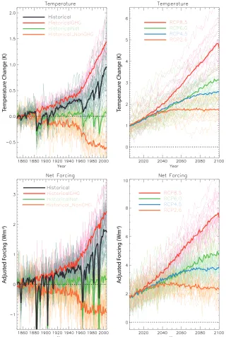
[10] Figure 2 shows the time evolution of globally

aver-aged surface temperature and calculated AF, relative to the preindustrial climate, for historical and future scenarios. The variation of AF across models and scenarios is shown in Figure 3. Figure 4 breaks down the components of AF in the models for year 2003 (2001–2005 average) and year 2095 (2090–2100 average).

[11] AFs and temperature changes for the individual

mod-els in these years are given in Tables 2 and 3 respectively. In the historical simulations, the 2003 AF (2001–2005 aver-age) was found to be 1.70.9 W m2 from the Historical

simulation, 2.40.8 W m2from theHistoricalGHG simu-lation, 0.10.2 W m2from theHistoricalNatsimulation, and 0.80.9 W m2 from theHistorical-nonGHG resi-dual simulation. This gives an anthropogenic (Historical

minusHistoricalNat) AF of 1.6 W m20.8 in 2003. All errors represent the 5%–95% model range. Multimodel mean

AFs for the RCP scenarios all depart from their expected RFs (Table 2 and Figure 2). RCP forcing estimates in 2095 are less than their targeted forcing, but agree very well with the forcing estimates derived from Integrated Assessment Modelling [Meinshausen et al., 2011]. When the different efficacies of the various forcing agents are accounted for, Mienshausen et al.find effective forcings in 2095 of 2.3, 3.9, 5.2, and 8.0 W m2for RCP2.6, RCP4.5, RCP6.0, and RCP8.5, respectively, within 10% of the CMIP5 model mean given in Table 2.

[12] The 5%–95% uncertainty range of AF in the Histori-calGHGsimulation in 2003 is0.8 W m2, which is nearly as large as the spread associated with nongreenhouse gas AF (Table 2). The evolution of net AF and surface temperature shows considerable spread among models (Figures 2 and 3). The fractional spread of net AF tends to grow much more in the historical period than in the future (Figure 3). Examining Figure 3a and Table 2, natural forcing differ-ences contribute least to the fractional model spread and greenhouse gas, and nongreenhouse gas forcing contribute in roughly equal proportions.

[13] Figure 4 examines the components of AF. The positive

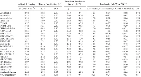
longwave (LW) clear-sky forcing is associated with greenhouse gas changes and has least spread between models. The cloud AF terms are calculated from anomalies in cloud radiative effect (CRE) where all-sky and clear-sky fluxes are differenced. Because radiative anomalies due to changes in forcing agents, water vapor, surface albedo, etc. are smaller in the presence of clouds than they would be in the absence of clouds, CRE-derived cloud AF estimates include a component of cloud masking. Model differences in aerosol forcings, rapid adjust-ments, and/or cloud masking effects can all contribute to the CRE-derived cloud AF spread. [Zelinka et al.,manuscript Table 1. CMIP5 Models Employed in This Paper and Their Feedback Components Computed

Adjusted Forcing Climate Sensitivities (K)

Transient Feedbacks

(W m2K1)a Feedbacks (a) (W m2K1)

2CO2 (W m2) ECS TCR r Κ LW clear sky SW clear sky Cloud: CRE derived Net

ACCESS1-0 2.98 3.83 2.00 1.49 0.71 1.63 0.77 0.08 0.78

bcc-csm1-1 3.23 2.82 1.70 1.90 0.76 1.91 0.83 0.07 1.14

bcc-csm1-1-m 3.55 2.87 2.10 1.69 0.45 1.98 0.68 0.06 1.24

CanESM2 3.84 3.69 2.40 1.60 0.56 1.88 0.71 0.13 1.04

CCSM4 3.57 2.89 1.80 1.98 0.75 1.95 0.87 0.16 1.23

CNRM-CM5 3.72 3.25 2.10 1.77 0.63 1.73 0.78 0.20 1.14

CSIRO-Mk3-6-0 2.59 4.08 1.80 1.44 0.81 1.70 0.84 0.23 0.63

FGOALS-s2 3.85 4.17 2.40 1.60 0.68 1.46 1.02 0.48 0.92

GFDL-CM3 2.99 3.97 2.00 1.50 0.75 1.94 0.70 0.48 0.75

GFDL-ESM2G 3.09 2.39 1.10 2.81 1.52 1.65 0.61 0.26 1.29

GFDL-ESM2M 3.36 2.44 1.30 2.58 1.20 1.63 0.58 0.33 1.38

GISS-E2-H 3.81 2.31 1.70 2.24 0.59 1.67 0.49 0.47 1.65

GISS-E2-R 3.78 2.11 1.50 2.52 0.73 1.66 0.36 0.48 1.79

HadGEM2-ES 2.93 4.59 2.50 1.17 0.53 1.66 0.65 0.37 0.64

inmcm4 2.98 2.08 1.30 2.29 0.86 1.98 0.67 0.12 1.43

IPSL-CM5A-LR 3.10 4.13 2.00 1.55 0.80 1.99 0.53 0.70 0.75

IPSL-CM5B-LR 2.66 2.61 1.50 1.77 0.75 1.88 0.59 0.28 1.02

MIROC5 4.13 2.72 1.50 2.75 1.23 1.85 0.84 0.51 1.52

MIROC-ESM 4.26 4.67 2.20 1.93 1.02 1.93 0.83 0.19 0.91

MPI-ESM-LR 4.09 3.63 2.00 2.05 0.92 1.79 0.71 0.04 1.13

MPI-ESM-P 4.31 3.45 2.00 2.16 0.91 1.80 0.65 0.10 1.25

MRI-CGCM3 3.25 2.60 1.60 2.03 0.78 1.99 0.83 0.09 1.25

NorESM1-M 3.11 2.80 1.40 2.22 1.11 1.86 0.86 0.11 1.11

Multimodel mean 3.44 3.22 1.82 1.96 0.83 1.81 0.71 0.04 1.13

90% uncertainty 0.84 1.32 0.63 0.73 0.41 0.25 0.24 0.53 0.51

a_{1% CO}

in revision, 2012]. A LW cloud masking effect of roughly +0.6 W m2 is expected from a doubling of CO2 [Andrews

and Forster, 2008;Soden et al., 2008;Colman and McAvaney, 2011]. We adopt the sign convention that the cloud masking effect represents an additional positive forcing that needs to be added to CRE-derived terms. As the forcing from CO2 is

currently around half of its doubled CO2value, this suggests

that around +0.3 W m2of cloud masking needs to be added to theHistoricalCRE-derived cloud AF terms. The RCP 8.5 CRE-derived cloud AF would need to have a larger compo-nent of masking added, around +0.6 W m2. The shortwave (SW) clear-sky AF and CRE-derived cloud AF split would

also be affected by cloud masking of sea-ice changes. Nevertheless, a negative CRE-derived cloud AF beyond that which is expected from cloud masking is seen in all the scenarios in Figure 4.

[14] The Historical-nonGHG AF shows a generally

negative trend that turned weakly positive around 1990 in most models (Figures 2 and 3), although some models show a strongly negative AF and others have an AF near zero or slightly positive (Figure 3). Because of the multiple forcing agents represented in the Historical-nonGHGscenario, the CMIP5 model spread in its AF of 0.80.9 W m2 in 2003 is difficult to interpret (see section 4).

4. Comparing Forcing Definitions

[15] In order to interpret the AFs given in section 3, it is

important to understand their uncertainty. Here we test three aspects of the analysis: (1) limitations of the two step AF process, (2) representing cloud AF using CRE-derived AFs, and (3) using the Historical-nonGHG scenario as a proxy for aerosol AF.

4.1. Limitations of the Two-step AF Process

[16] FT06 found that forcings from the two-step regression

procedure agreed with offline RF calculations in two models. However, variation in climate sensitivity could in principle bias the AF estimates. While some bias cannot be ruled out, for a scenario with CO2increasing at 1% per year, ensemble

mean AF (derived using the FT06-updated method) has been found to increase linearly with time (to within the precision set by internal variability), as expected if climate sensitivity were approximately constant [Good et al., 2012]. To test this further, we compared the FT06-updated AF with an AF de-rived from transient experiments where SSTs are prescribed from observations [Held et al., 2010]. The SST-derived method used two transient integrations, one with forcing agents and one without. The run with changes in forcing agents gives a heat balance described by equation (1), and the run without changes in forcing agents gives a heat balance described by (note the primes):

N0¼F0aΔT0 (2)

where F0= 0 by definition. As SSTs are identically prescribed in both,ΔT ~ΔT0, and substituting equation (2) into equation (1) gives:

F¼NN0 (3)

AFs derived from these two definitions are compared in Figure 5. Although there is considerable variability in the FT06-updated AF, its AF seems to agree very well with the prescribed SST-derived AF from a 10-ensemble member

Figure 3. (a) Time series of AF from the different historical scenarios. (b) Time series of AF from the different future scenarios.

-4 -2 0 2 4 6 8 10 12 LW clear-sky

SW clear-sky

Cloud (CRE derived)

NET

Adjusted Forcing (Wm-2₎ Historical in 2003

HistoricalGHG in 2003

RCP8.5 in 2095

Figure 4. Diagnosed AFs (since preindustrial) for the

average in this one CMIP3 model. The AFs calculated from the two methods could diverge if the integration continued beyond 2000 out to 2100. Nevertheless, this comparison gives some confidence that differences between the FT06-updated AF and other AF estimates are comparable and not affected by an error associated with possible climate sensitivity drift with the FT06-updated methodology.

4.2. Representing Cloud AF Using CRE-derived AFs

[17] To test the CRE-derived AF estimates and examine if

they arise from a rapid adjustment of cloud or from cloud masking, cloud-induced radiation anomalies can be computed directly from cloud anomalies diagnosed by the ISCCP simu-lator [Klein and Jakob, 1999;Webb et al., 2001] in combina-tion with cloud radiative kernels [Zelinka et al., 2012]. The kernels quantify the impact on TOA radiativefluxes of cloud fraction perturbations for each of the 49 different ISCCP simu-lator cloud types. Multiplying cloud fraction anomalies by the kernels yields TOA radiation anomalies that are purely a result of cloud changes and are free of any noncloud effects. There-fore, we refer to the cloud AFs and feedbacks that are computed from these cloud-induced anomalies as“unmasked,”to be dis-tinguished from those derived using CRE, which include mask-ing effects.

[18] To derive cloud AFs, we follow the exact same

FT06-updated procedure as described in section 2, but replace N in equation (1) with cloud-induced radiativeflux anomalies, so thatais the unmasked cloud feedback. The unmasked cloud feedbackaterms are derived from the abrupt 4xCO2runs in

Zelinka et al. [manuscript under revision 2012] for the five models that have archived the necessary diagnostics. The CRE-derived and unmasked LW, SW, and net cloud AFs in 2003 for the Historical run are compared in Figure 6. As expected, the unmasked LW cloud AF is systematically more positive than the CRE-derived value in every model (0.56 W m2 larger on average), and the unmasked SW cloud AF is systematically less positive or more negative than the CRE-derived value (0.32 W m2smaller on aver-age). This brings the unmasked negative net cloud AF in 2003 closer to zero (0.33 rather than0.57 W m2) and

Table 2. AFs for Different Scenarios Given at 2003 (2001–2005 Average), 2010 (2008–2012 Average), and 2095 (2091 to 2099)

Adjusted Forcing (W m2) for Scenario and Period

Hist 2003

HistGHG 2003

HistNat 2003

Hist NonGHG 2003

RCP 4.5 2010

RCP2.6 2095

RCP4.5 2095

RCP6.0 2095

RCP8.5 2095

ACCESS1-0 1.1 1.4 3.3 6.2

bcc-csm1-1 2.2 2.0 0.1 0.0 2.0 2.5 3.3 4.5 7.0

bcc-csm1-1-m 2.2 2.2 1.9 3.3 4.3 7.0

CanESM2 2.0 2.4 0.1 0.5 2.2 2.9 4.3 8.4

CCSM4 2.5 2.3 0.1 0.1 2.7 2.8 4.3 5.4 8.3

CNRM-CM5 1.5 2.2 0.1 0.8 1.2 2.3 3.7 6.9

CSIRO-Mk3-6-0 0.9 1.4 0.1 0.6 1.0 1.9 2.8 3.4 5.7

FGOALS-s2 2.3 2.8 2.5 4.3 6.5 10.0

GFDL-CM3 1.1 2.9 0.5 2.2 1.7 3.1 4.2 4.9 7.2

GFDL-ESM2G 2.0 1.9 1.2 2.8 3.9 6.4

GFDL-ESM2M 2.0 2.5 0.2 0.7 2.2 2.5 3.5 4.9 7.3

GISS-E2-H 2.3 3.2 0.2 1.0

GISS-E2-R 2.5 3.3 0.2 0.9 2.5 2.6 4.7 5.9 8.6

HadGEM2-ES 0.8 1.9 0.1 1.1 1.0 1.7 2.9 4.0 5.9

inmcm4 1.7 1.9 3.8 7.3

IPSL-CM5A-LR 1.9 2.4 0.2 0.7 1.8 2.2 3.5 4.3 7.1

IPSL-CM5B-LR 1.0

MIROC5 1.6 2.0 3.0 4.5 5.3 8.7

MIROC-ESM 1.1 2.2 0.0 1.0 1.5 2.8 4.0 5.1 8.2

MPI-ESM-LR 2.1 2.3 2.2 3.9 7.7

MPI-ESM-P 2.3

MRI-CGCM3 1.2 2.1 0.2 1.1 1.2 2.1 3.6 4.3 7.0

NorESM1-M 1.4 2.3 0.0 0.9 1.7 2.0 3.6 4.2 7.0

Multimodel mean

1.7 2.4 0.1 0.8 1.9 2.3 3.7 4.7 7.4

90% uncertainty

0.9 0.8 0.2 0.9 0.9 0.8 0.9 1.3 1.8

increases the spread in this quantity among thefive models. That the unmasked net cloud AF is nonzero indicates that cloud rapid adjustments are physically occurring and are tending to reduce the effective climate forcing. The differ-ence between the unmasked and CRE-derived cloud AFs quantifies the amount of cloud masking in the section 3 esti-mates of AF. The net cloud masking effect at the end of the

Historical run in these 5 models is systematically positive

and averages to 0.24 W m2. In agreement with expectations from section 3, this is roughly half of the value expected for doubling of CO2.

[19] The SW cloud AF dominates over the LW cloud AF

in every model, in agreement with previous studies. How-ever, Zelinka et al. [manuscript under revision, 2012] find a positive unmasked SW rapid adjustment cloud AF under 4xCO2 for all five models, which raises the question of

why most (three out of these five) models give negative unmasked SW cloud AFs in 2003 given that CO2 is the

dominant forcing agent in the latter part of the Historical

run. This may be evidence that the non-CO2forcing agents

(which are present in theHistoricalrun but not in the ideal-ized 4xCO2runs) cause significant cloud adjustments, even

if they are not the ones responsible for most of the unad-justed forcing (just like cloud feedbacks are responsible for most of the spread in climate feedback, whereas water vapor is responsible for most of the ensemble mean feedback). Pre-vious studies have found large cloud forcing from rapid adjustments associated with perturbations to the solar con-stant, black carbon, and ozone [e.g., Hansen et al., 2005;

Bala et al., 2009;Ban-Weiss et al., 2011], but these cloud forcing vary considerably between the location and magni-tude of the forcing agent and the model. On the other hand, our diagnosed cloud AF could be an artefact of the assump-tions inherent in the two-step regression technique.

4.3. Using theHistorical-nonGHGScenario as a Proxy for Aerosol AF

[20] To test the aerosol AF estimate, we examinedfi

xed-SST experiments existing in the CMIP5 archive. In these experiments, individual forcing agents have been intro-duced; present-day aerosol perturbation experiments exist

−2 −1.5 −1 −0.5 0 0.5 1

SW

LW

Net

Cloud Adjusted Forcing, 2003

Adjusted Forcing (W m−2)

CRE−derived Unmasked Masking

Figure 6. Multimodel mean and standard deviation of the global-mean cloud AFs for the unmasked (i.e., cloud kernel-derived) AF and CRE-derived AF. Cloud AFs are given for LW, SW, and net variables forfive GCMs averaged over years 2001–2005 of the Historical simulations. Unmasked minus CRE-derived cloud AFs gives an estimate of the cloud mask-ing of the forcmask-ing.

Table 3. Temperature Changes Since Preindustrial Times for Different Scenarios Given at 2003 (2001–2005 Average), 2010 (2008–2012 Average), and 2095 (2091 to 2099)

Temperature Change Since Preindustrial (K) for Scenario and Period

Hist 2003

Hist GHG 2003

Hist Nat 2003

Hist NonGHG 2003

RCP 4.5 2010

RCP2.6 2095

RCP4.5 2095

RCP6.0 2095

RCP8.5 2095

ACCESS1-0 0.6 0.8 2.7 4.8

bcc-csm1-1 1.2 1.4 0.1 0.3 1.4 2.0 2.5 3.1 4.6

bcc-csm1-1-m 1.7 1.8 2.0 2.7 3.2 4.8

CanESM2 1.0 1.6 0.1 0.4 1.2 2.3 3.2 5.5

CCSM4 1.3 1.3 0.0 0.1 1.3 1.9 2.7 3.2 4.7

CNRM-CM5 1.0 1.3 0.1 0.4 1.1 1.8 2.7 4.5

CSIRO-Mk3-6-0 0.7 1.2 0.2 0.7 0.7 1.9 2.5 2.9 4.8

FGOALS-s2 1.8 2.0 2.1 3.0 4.4 6.6

GFDL-CM3 0.3 1.8 0.1 1.4 0.9 2.1 2.9 3.5 5.1

GFDL-ESM2G 0.8 1.0 0.8 1.6 2.2 3.6

GFDL-ESM2M 0.8 1.0 0.0 0.2 0.8 1.3 1.8 2.3 3.5

GISS-E2-H 1.2 1.4 0.1 0.3

GISS-E2-R 1.1 1.2 0.2 0.3 1.1 1.4 2.2 2.6 3.7

HadGEM2-ES 0.5 1.5 0.0 1.0 0.7 1.7 2.8 3.6 5.2

inmcm4 0.8 0.9 2.0 3.5

IPSL-CM5A-LR 1.4 1.9 0.2 0.7 1.5 2.3 3.3 3.8 5.8

IPSL-CM5B-LR 0.9

MIROC5 0.6 0.8 1.4 2.1 2.5 4.0

MIROC-ESM 0.7 1.3 0.0 0.6 1.0 2.3 3.1 3.7 5.5

MPI-ESM-LR 1.0 1.2 1.5 2.5 4.6

MPI-ESM-P 1.0

MRI-CGCM3 0.6 1.1 0.1 0.6 0.5 1.3 2.1 2.4 3.9

NorESM1-M 0.7 1.2 0.1 0.4 1.0 1.4 2.2 2.5 4.0

Multimodel mean 1.0 1.4 0.1 0.5 1.1 1.8 2.5 3.1 4.6

for three models, and their AFs can be compared to the FT06-updated AFs, taken from the Historical-nonGHG

simulations. Thefixed-SST AFs are taken as the difference of TOAfluxes between a forced and a preindustrial control experiment (as in equation (3)). These AFs are given in Table 4, which also shows AFs from the FT06-updated method, repeated from Table 2. The AFs derived by the two methods are appreciably different, indicating that other nongreenhouse forcing agents, such as land-use and ozone, as well as the aerosol signal affect theHistorical-nonGHG

simulations.

[21] This section has shown that it is not appropriate to

represent aerosol AF by the Historical-nonGHG residual scenario and that CRE-derived cloud AFs may not be rep-resentative of actual AFs from rapid cloud adjustment. Nevertheless the net AF does correctly capture both RF and cloud adjustment and could be expected to match other AF estimates over 1850–2100 simulations and can there-fore provide useful insights into the causes of global-mean temperature change, examined next.

5. Intermodel Temperature Spread

[22] This section uses the AFs diagnosed in section 3 to help

understand the gross characteristics of the CMIP5 models’ surface temperature response. In particular, we focus on how differences in forcing and climate sensitivity affect the inter-model spread of surface temperature change.

[23] A model’s historical temperature trend depends on

forcing, climate sensitivity, and ocean heat uptake. As aerosol forcing and climate sensitivity are uncertain, modeling centers could be modifying their controlling factors to reproduce the observed globally averaged 20th century temperature trends as well as possible. There was some evidence of a trade off between climate sensitivity and forcing in CMIP3 and earlier generations of models [Kiehl, 2007;Knutti, 2008]. Figure 7 reproduces Figure 1 ofKiehl[2007] for CMIP5 models and finds considerably smaller correlation than in either the CMIP3 analysis ofKnutti[2008] or the older model analysis ofKiehl[2007] that are reproduced as blue and red symbols, respectively. The R2fit in CMIP5 models is slightly smaller than in CMIP3 models and is not significant. The green squares show a subset of the CMIP5 models that match the observed century-scale linear temperature trends (0.57 to 0.92 K increase over 1906–2006,IPCC[2007]). This subset reproduces theKiehl[2007]fit almost perfectly. The CMIP5

models that are not in this grouping tend to have a larger positive AF compared to those that match observations and thereby overestimate the observed temperature trend. Varia-tion in the magnitude of the CO2AF affects both the AF in

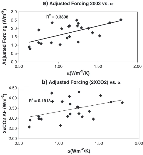
2003 and the equilibrium climate sensitivity (ECS). Figure 8 shows that both AF in 2003 and the 2xCO2AF are positively

R² = 0.3898

0.0 0.5 1.0 1.5 2.0 2.5 3.0

0.50 1.00 1.50 2.00

-2

/K)

(Wm-2/K) R² = 0.1913

2.00 2.50 3.00 3.50 4.00 4.50

0.50 1.00 1.50 2.00

Adjusted Forcing (Wm

-2 )

2xCO2 AF (Wm

-2 )

(Wm

a) Adjusted Forcing 2003 vs.

b) Adjusted Forcing (2XCO2) vs.

Figure 8. Scatterplots of (a) Historical 2003 AF against

aand (b) 2xCO2AF againsta.

Kiehl: R² = 0.5027 CMIP3 (Knutti):R² = 0.2414

CMIP5: R² = 0.1941 CMIP5 selection: R² = 0.7369

0.0 0.5 1.0 1.5 2.0 2.5 3.0

1.8 2.3 2.8 3.3 3.8 4.3 4.8 5.3

Adjusted Forcing (Wm

-2 )

Equilibrium Climate Sensitivity (K)

Adjusted Forcing in 2003 vs. Equilibrium Climate Sensitivity (K)

Figure 7. The relationship between 2003 AF and ECS in CMIP5 and earlier generations of models. CMIP3 numbers are taken fromKnutti[2008] and older models from Kiehl

[2007]. The solid linefits are made using the inverse rela-tionship between forcing and climate sensitivity postulated byKiehl [2007]. Data are shown for all CMIP5 models as black diamonds, using the Historical simulation. A subset of CMIP5 models is shown by the green squares that are within the 90% uncertainty range of the observed 100 year linear temperature trend. These models have 1906–2005 linear trends between 0.56 K and 0.92 K, the IPCC[2007] 90% uncertainty range. R2values are computed with respect to the nonlinearfit shown.

Table 4. AFs Calculated for Aerosol-only Perturbations in Fixed-SST Experiments Compared to AFs for 2003 From the FT06-updatedHistorical-nonGHGResidual Scenario

Model

Net Clear Sky Cloud: CRE Derived

Forcing (W m2)

Fixed SST

CanESM2 0.86 0.59 0.28

CSIRO-Mk3 1.41 1.04 0.37

HadGEM2-ES 1.23 0.35 0.88

FT06-updated residual

CanESM2 0.51 0.33 0.18

CSIRO-Mk3 0.61 0.59 0.02

correlated witha[see alsoAndrews et al., 2012b]. This means that models with smaller climate feedbacks (i.e., higher sensi-tivities) tend to also have smaller CO2AFs which would act to

converge models towards similar Historical temperature responses.

[24] The transient response of a model depends on ocean

heat uptake as well as the ECS. If modelling groups are adjusting forcing to match the observed temperature trends then one might expect that the correlation between 2003 AF and the transient climate response (TCR) to be larger than the correlation between 2003 AF and ECS. However, these correlations are 0.11 and 0.41, respectively, and neither is significant at the 5% level.

[25] The causes of model spread can be further examined

by using the approach of Gregory and Forster [2008], whereby the global-mean temperature change under a sce-nario of continually increasing forcing is:

ΔT ¼F=r (4)

where the climate resistance r=a+k, k being the ocean heat uptake efficiency.

[26] The estimates ofrandkfrom the 1% per year CO2

in-crease simulations are given in Table 1. Theavalues used are derived from the 4xCO2abrupt integration from section 3 and

are also presented in Table 1. Theavalues derived from the 1% per year CO2increase integration (not shown) were very

similar to values diagnosed from the 4xCO2abrupt integration

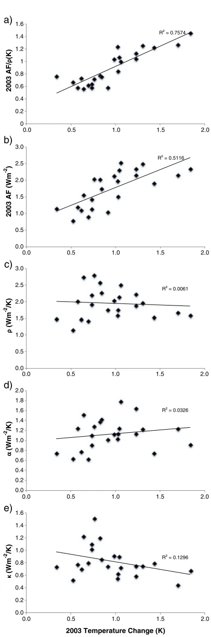
[see alsoKuhlbrodt and Gregory, 2012]. Figure 9 examines how AF in 2003,r,a, andkinfluence the temperature change. As expected, AF /r(Figure 9a) explains most of the variation in temperature, and AF (Figure 9b) is by far the most impor-tant influence. Models with aHistorical AF in 2003 that is more positive than about 2 W m2typically have a tempera-ture change that is larger than observed. In contrast, r, a, andk(Figures 9c, 9d, and 9e) show no systematic tendency for affecting temperature. For example, the HadGEM2-ES and GFDL-CM3 models exhibit two of the smallest tempera-ture changes but also have two of the smallestavalues (high ECS). Therefore, their small temperature change results pri-marily from a small forcing. These results suggest that AF in some models may be too positive to accurately reproduce historic temperature trends.

[27] Multiple linear regression was used to model the

CMIP5 spread of temperatures using explanatory variables of AF,a,r, andkfrom Tables 1 and 2. Of these, the strongest correlation was found between AF in 2003 andaat 0.62 (see Figure 8a).randkwere somewhat positively correlated with F, but not by as much (0.45 and 0.02 respectively). These cor-relations mean that whilst models with larger AF generally have larger feedback parameters (smaller sensitivities) and more efficient ocean heat uptake (largerk), no clear pattern of compensation emerges between climate model feedback parameters, or ocean heat uptake, and AF (see also Figure 9). [28] Figure 10 comparesrderived from two RCPs with

in-creasing forcing over 2000–2050, withrderived from the 1% per year CO2increase simulation that is used to define TCR.

Estimates of r are generally well correlated between the RCP scenarios and the 1% per year CO2increase simulation.

kvalues are not shown but follow a similar pattern. The 1% per year run has a larger forcing increase than RCP 8.5, and models have a consistently largerkandrfor this scenario than

R² = 0.7574

0 0.2 0.4 0.6 0.8 1 1.2 1.4 1.6

0.0 0.5 1.0 1.5 2.0

R² = 0.5116

0.0 0.5 1.0 1.5 2.0 2.5 3.0

0.0 0.5 1.0 1.5 2.0

R² = 0.0061

0.0 0.5 1.0 1.5 2.0 2.5 3.0

0.0 0.5 1.0 1.5 2.0

R² = 0.0326

0.0 0.2 0.4 0.6 0.8 1.0 1.2 1.4 1.6 1.8 2.0

0.0 0.5 1.0 1.5 2.0

R² = 0.1296

0.0 0.2 0.4 0.6 0.8 1.0 1.2 1.4 1.6

0.0 0.5 1.0 1.5 2.0

2003 AF/

(K)

2003 AF (Wm

-2 ) (Wm -2 /K) (Wm -2 /K) (Wm -2 /K)

2003 Temperature Change (K)

d) c) b) a)

e)

Figure 9. Scatterplots of (a) AF/r, (b) AF, (c)r, (d)a, and (e)

kagainst the temperature change in 2003 from theHistorical

those derived from the other scenarios. Likewise, RCP8.5, compared to RCP 4.5 has a larger forcing increase and larger

kandrover the period. A more rapid forcing increase would be better at maintaining stronger vertical temperature gradients within the ocean. These would be expected to be more effi -cient at transferring heat from the surface to the subsurface ocean, leading to a largerkand, therefore, a largerrvalue.

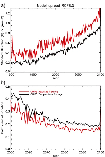
[29] Figure 11a shows how the standard deviation in AF

and temperature change projections between models varies with time for the RCP 8.5 scenario. Note the similarity of the two quantities, consistent with the expectation from equation (4) that temperature change is proportional to AF if climate resistance is constant. The coefficient of variation (standard deviation/mean) is largest for the present day (Figure 11b) because the standard deviation does not grow as rapidly as the model mean.

[30] Multiple linear regression was performed on the

model temperature change in 2010 and 2095, regressing the temperature change across models against their AF in the same year anda. Examining model spread, an across-model regression of temperature change simultaneously againstaand AF gave a goodfit to the data for both 2010 and 2095 (see Figure 12). In RCP4.5, this regression explained 72% of the variation in temperature change and slope coeffi -cients for both AF andawere statistically significant at the 0.1% significance level. For 2010 data, AF explained the larg-est proportion of variation in the temperature change (49%) withaimproving thefit across the full range of temperature changes. In contrast,aexplained the largest proportion of var-iation in the temperature change in the 2095 data (42%) with

0.6 0.8 1.0 1.2 1.4 1.6 1.8

Temperature Change in 2010

Fitted values of Temperature Change (K)

Temperature Change (K)

R2 0.64

2.0 2.5 3.0

0.5

1.0

1.5

2.0

1.5

2.0

2.5

3.0

R2 0.72

Temperature Change in 2095

Fitted values of Temperature Change (K)

Temperature Change (K)

Figure 12. Modeled temperature changes for 2010 and 2095 for the RCP 4.5 scenario, compared to fitted values from the linear regression. The red line represents the 1:1 re-lationship. Thefitted values are for the linear regression with bothaand AF included as explanatory variables.

a)

b)

Figure 11. The (a) standard deviation and (b) coefficient of variation (standard deviation/mean) between models for tem-perature (black) and AF (red) as a function of time for the

RCP8.5scenario. Note the different time scales on the x axis.

0.8 1.3 1.8 2.3 2.8 3.3

1.0 1.5 2.0 2.5 3.0

(Wm

-2 /K) from 2000-2050 trends

(Wm-2/K) from 1% CO₂ per year increase

RCP 4.5

RCP 8.5

1:1 line

Figure 10. Resistance (r) derived from 2000–2050 trends in theRCP 4.5andRCP 8.5scenarios compared to those derived for the 1% per year CO2increase scenario that is used to

forcing improving thefit particularly for data points with more extreme (both large and small) temperature changes. Tempe-rature change is much more sensitive to variations inain the 2095 data than in the 2010 data, with a regression slope coef-ficient of 1.450.22 for 2095 compared to 0.560.21 for 2010. There was no significant difference in sensitivity to AF between 2010 and 2095.

[31] This analysis shows that large forcing differences

be-tween models today give a large spread in model tempera-ture change. This is partly due to the current strong aerosol forcing that varies considerably between models, but this aerosol forcing is projected to weaken. Any relationship be-tweenaand AF has little effect on model spread, and there is no indication of models herding towards similar 20th cen-tury temperature trends. In the future, the role of forcing remains important, and, therefore, differences in forcing will need to be considered when comparing model simulations within a given scenario.

6. Discussion and Conclusions

[32] The estimated anthropogenic AF of 1.6 W m20.9

and the estimated greenhouse gas AF of 2.40.8 W m2 in 2003 agree well with the last IPCC report and more recent estimates of RF, even though the definition of the two for-cings differ. For example,Forster et al. [2007] estimated a total anthropogenic forcing of 1.61.0 W m2 in 2005, and Skeie et al. [2011] estimated a year 2000 greenhouse gas RF of 2.5 W m2.

[33] The total AF from CMIP5 models, estimated to be

1.70.9 W m2 in 2003, grows to 1.90.9 W m2 in 2010. In contrast to the 2007 IPCC estimate, where the spread was principally attributed to aerosols, the spread found here comes from both nongreenhouse gas forcing agents and differences in the rapid adjustment of cloud to greenhouse gases.

[34] The AF estimates made in this paper include a signifi

-cant cloud component that acts to make the AF smaller than the expected RF. Because of this, the projected 2095 AFs are lower than the corresponding estimate of RF from the original RCP scenario. However, they agree well with the effective forc-ing estimate of the integrated assessment models [Meinshausen et al., 2011]. Consistent with a lower AF, Andrews et al. [2012b] found that CMIP5 models had a 4xCO2AF that ranged

between 5.6 and 8.5 W m2and was, on average, 0.4 W m2 lower than the expected RF of 7.4 W m2. Figures 1 and 3 in

Andrews et al. [2012b] suggest that rapid adjustments within this framework are not necessarily an immediate physical cloud change but could also be associated, in some AOGCMs, with a nonlinear response in SW CRE principally found over oceans. This is further supported inZelinka et al. [manuscript in prepa-ration, 2012] who show that unmasked cloud AFs diagnosed using this linear framework (i.e., the linear regression line inter-cept) tend to be negatively biased with respect to those diag-nosed in fixed SST and perturbed CO2 simulations. These

caveats limit our ability to interpret RF and AF differences as a genuine cloud adjustment.

[35] Generally, it would be useful to test the FT06-updated

approach under a wider set of models and scenarios to better quantify and understand its errors, quantify differ-ences with other AF methodologies, and quantify the role of rapid adjustment.

[36] Issues remain around the definitions of AF and the

assumption of constant climate sensitivity within a transient forcing framework. The forcing/climate sensitivity concept developed essentially for slab-ocean models at equilibrium obviously does not provide a complete picture of climate evolution in today’s nonlinear AOGCMs. Nevertheless, we argue that forcings are useful for understanding why models differ in their gross behavior and forcings explain the spread of RCP projections rather well. Careful analysis of the Earth’s energy budget examining climate response on multi-ple timescales is recommended.

[37] Acknowledgments. PF was supported by EPSRC grant EP/ I014721/1 and A Royal Society Wolfson Merit Award. We acknowledge the World Climate Research Program’s Working Group on Coupled Modelling, which is responsible for CMIP, and we thank the climate modelling groups (listed in Table 1 of this paper) for producing and making available their model output. For CMIP, the U.S. Department of Energy’s Program for Climate Model Diagnosis and Intercomparison provides coordinating support and led development of software infra-structure in partnership with the Global Organization for Earth System Science Portals. TA and JG were supported by the Joint DECC/Defra Met Office Hadley Center Climate Program (GA01101). We thank Isaac Held for providing the forcing data fromHeld et al. [2010]. The contribu-tion of MDZ was performed under the auspices of the U.S. Department of Energy by Lawrence Livermore National Laboratory (LLNL) under Contract DE-AC52-07NA27344 and was supported by the LLNL Institutional Postdoctoral Program. Very helpful review comments were provided by Jeff Kiehl, and two anonymous reviewers.

References

Andrews, T., and P. M. Forster (2008), CO2forcing induces semi-direct effects with consequences for climate feedback interpretations,Geophys. Res. Lett.,35, L04802.

Andrews, T., P. M. Forster, O. Boucher, N. Bellouin, and A. Jones (2010), Precipitation, radiative forcing and global temperature change,Geophys. Res. Lett.,37, L14701.

Andrews, T., J. M. Gregory, P. M. Forster, and M. J. Webb (2012a), Cloud adjustment and its role in CO2 radiative forcing and climate sensitivity: A review,Surv. Geophys.,33, 619–635, doi:10.1007/s10712-011-9152-0.) Andrews, T., J. M. Gregory, M. J. Webb, and K. E. Taylor (2012b), Forcing,

feedbacks and climate sensitivity in CMIP5 coupled atmosphere–ocean climate models,Geophys. Res. Lett.,39, L09712.

Ban-Weiss, G. A., L. Cao, G. Bala, and K. Caldeira (2011), Dependence of climate forcing and response on the altitude of black carbon aerosols, Clim. Dynam., doi:10.1007/s00382-011-1052-y.

Bala, G., K. Caldeira, and R. Nemani (2009), Fast versus slow response in climate change: Implications for the global hydrological cycle, Clim. Dynam.,35, 423–434.

Collins, W. D., et al. (2006), Radiative forcing by well-mixed greenhouse gases: Estimates from climate models in the Intergovernmental Panel on Climate Change (IPCC) Fourth Assessment Report (AR4),J. Geophys. Res.,111, D14317.

Colman, R. A., and B. J. McAvaney (2011), On tropospheric adjustment to forcing and climate feedbacks,Clim. Dynam.,36(9–10), 1649–1658. Dong, B. W., J. M. Gregory, and R. T. Sutton (2009), Understanding

land-sea warming contrast in response to increasing greenhouse gases. Part I: Transient adjustment,J. Clim.,22(11), 3079–3097.

Forster, P. M., and K. Taylor (2006), Climate forcings and climate sen-sitivities diagnosed from coupled climate model integrations, J. Clim., 6181–6194.

Forster, P., et al. (2007), Changes in Atmospheric Constituents and in Radiative Forcing, inClimate Change 2007: The Physical Science Basis. Contribution of Working Group I to the Fourth Assessment Report of the Intergovernmental Panel on Climate Change, edited by S. Solomon, D. Qin, M. Manning, Z. Chen, M. Marquis, K. B. Averyt, M. Tignor, and H. L. Miller, Cambridge University Press, Cambridge, UK and New York, NY.

Forster, P. M., et al. (2011), Evaluation of radiation scheme performance within chemistry climate models, J. Geophys. Res., 116, D10302, doi:10.1029/2010JD015361.

representative concentration pathway projections, Clim. Dynam., doi:10.1007/s00382-012-1410-4.

Gregory, J. M., W. Ingram, M. Palmer, G. Jones, P. Stott, R. Thorpe, J. Lowe, T. Johns, and K. Williams (2004), A new method for diagnosing radiative forcing and climate sensitivity,Geophys. Res. Lett.,31, L03205. Gregory, J. M., and P. Forster (2008), Transient climate response estimated from radiative forcing and observed temperature change, J. Geophys. Res.,113, D23105.

Gregory, J. M., and M. Webb (2008), Tropospheric adjustment induces a cloud component in CO2forcing,J. Clim.,21(1), 58–71.

Hansen, J., et al. (2005), Efficacy of climate forcings,J. Geophys. Res.,110, D18104, doi:10.1029/2005JD005776.

Held, I., M. Winton, K. Takahashi, T. Delworth, F. Zeng, and G. Vallis (2010), Probing the fast and slow components of global warming by returning abruptly to preindustrial forcing,J. Clim.,23(9), 2418–2427. IPCC (2007), Climate Change 2007: The Physical Science Basis.

Contribu-tion of Working Group I to the Fourth Assessment Report of the Intergov-ernmental Panel on Climate Change [Solomon, S., D. Qin, M. Manning, Z. Chen, M. Marquis, K. B. Averyt, M. Tignor and H. L. Miller (eds.)]. Cambridge University Press, Cambridge, United Kingdom and New York, NY, USA, 996 pp.

Kiehl, J. T. (2007), Twentieth century climate model response and climate sensitivity,Geophys. Res. Lett.,34, L22710.

Klein, S. A., and C. Jakob (1999), Validation and sensitivities of frontal clouds simulated by the ECMWF model,Mon. Weather Rev.,127, 2514–2531. Knutti, R. (2008), Why are climate models reproducing the observed global

surface warming so well?Geophys. Res. Lett.,35, L18704.

Kuhlbrodt, T., and J. M. Gregory (2012), Ocean heat uptake and its conse-quences for the magnitude of sea level rise and climate change,Geophys. Res. Lett., doi:10.1029/2012GL052952, in press.

Lohmann, U., L. Rotstayn, T. Storelvmo, A. Jones, S. Menon, J. Quaas, A. M. L. Ekman, D. Koch, and R. Ruedy (2010), Total aerosol effect: Radiative forcing or radiativeflux perturbation?Atmos. Chem. Phys.,10(7), 3235–3246. Meinshausen, M., et al. (2011), The RCP greenhouse gas concentrations and

their extensions from 1765 to 2300,Clim. Chang.,109(1–2), 213–241. Ramaswamy, V., O. Boucher, J. Haigh, D. Hauglustaine, J. Haywood, G. Myhre,

T. Nakajima, G. Y. Shi, and S. Solomon (2001), Radiative Forcing of Climate Change, in Climate Change 2001: The Scientific Basis. Contribution of Working Group I to the Third Assessment Report of the Intergovernmental Panel on Climate Change, edited by J. T. Houghton, Y. Ding, D. J. Griggs, M. Noguer, P. J. van der Linden, X. Dai, K. Maskell and C. A. Johnson, Cambridge University Press, Cambridge, UK and New York, NY. Rotstayn, L. D., and J. E. Penner (2001), Indirect aerosol forcing, quasi

forcing, and climate response,J. Clim.,14(13), 2960–2975.

Shine, K., and P. Forster (1999), The effect of human activity on radiative forcing of climate change: a review of recent developments, Global Planet. Change, 205–225.

Skeie, R., T. Berntsen, G. Myhre, K. Tanaka, M. Kvalevag, and C. Hoyle (2011), Anthropogenic radiative forcing time series from pre-industrial times until 2010,Atmos. Chem. Phys.,11(22), 11827–11857.

Soden, B. J., I. M. Held, R. Colman, K. M. Shell, J. T. Kiehl, and C. A. Shields (2008), Quantifying climate feedbacks using radiative kernels, J. Clim.,21(14), 3504–3520.

Webb, M., C. Senior, S. Bony, and J. J. Morcrette (2001), Combining ERBE and ISCCP data to assess clouds in the Hadley Centre, ECMWF and LMD atmospheric climate models,Clim. Dynam.,17, 905–922. Zelinka, M. D., S. A. Klein, and D. L. Hartmann (2012), Computing and