Estimating Multiparameter Partial Expected Value of Perfect Information from a Probabilistic Sensitivity Analysis Sample: A Nonparametric Regression Approach

Universities of Leeds, Sheffield and York

http://eprints.whiterose.ac.uk/

This is a copy of the final published version of a paper published via gold open access

in

Medical Decision Making

.

This open access article is distributed under the terms of the Creative Commons

Attribution Licence (

http://creativecommons.org/licenses/by/3.0

), which permits

unrestricted use, distribution, and reproduction in any medium, provided the

original work is properly cited.

White Rose Research Online URL for this paper:

http://eprints.whiterose.ac.uk/78428

Published paper

Strong, M, Oakley, JE and Brennan, A (2013) Estimating Multiparameter Partial

Expected Value of Perfect Information from a Probabilistic Sensitivity

http://mdm.sagepub.com/

Medical Decision Making

http://mdm.sagepub.com/content/34/3/311

The online version of this article can be found at:

DOI: 10.1177/0272989X13505910

2014 34: 311 originally published online 18 November 2013

Med Decis Making

Mark Strong, Jeremy E. Oakley and Alan Brennan

Analysis Sample: A Nonparametric Regression Approach

Estimating Multiparameter Partial Expected Value of Perfect Information from a Probabilistic Sensitivity

Published by:

http://www.sagepublications.com

can be found at:

Medical Decision Making

Additional services and information for

Immediate free access via SAGE Choice

Open Access:

http://mdm.sagepub.com/cgi/alerts Email Alerts:

http://mdm.sagepub.com/subscriptions Subscriptions:

http://www.sagepub.com/journalsReprints.nav Reprints:

http://www.sagepub.com/journalsPermissions.nav Permissions:

What is This?

- Nov 18, 2013

OnlineFirst Version of Record

- Mar 31, 2014

Version of Record

Estimating Multiparameter Partial Expected

Value of Perfect Information from

a Probabilistic Sensitivity Analysis Sample:

A Nonparametric Regression Approach

Mark Strong, PhD, Jeremy E. Oakley, PhD, Alan Brennan, PhD

The partial expected value of perfect information (EVPI) quantifies the expected benefit of learning the values of uncertain parameters in a decision model. Partial EVPI is commonly estimated via a 2-level Monte Carlo procedure in which parameters of interest are sampled in an outer loop, and then conditional on these, the remaining parame-ters are sampled in an inner loop. This is computationally demanding and may be difficult if correlation between input parameters results in conditional distributions that are hard to sample from. We describe a novel nonparametric regres-sion-based method for estimating partial EVPI that requires only the probabilistic sensitivity analysis sample (i.e., the set of samples drawn from the joint distribution of the

parameters and the corresponding net benefits). The method is applicable in a model of any complexity and with any specification of input parameter distribution. We describe the implementation of the method via 2 nonpara-metric regression modeling approaches, the Generalized Additive Model and the Gaussian process. We demonstrate in 2 case studies the superior efficiency of the regression method over the 2-level Monte Carlo method. R code is made available to implement the method.Key words:value of information; expected value of perfect information; eco-nomic evaluation model; nonparametric regression; Bayes-ian decision theory; computational methods. (Med Decis Making 2014;34:311–326)

H

competing decision options. The true values of the input parameters of such models are rarely known with certainty, and it is often useful to quantify the value to the decision maker of reducing uncertainty about the model input parameters. The value of learning an input parameter (or a group of input parameters) can be quantified by its partial expected value of perfect information (partial EVPI).1–4 The partial EVPI value for an input parameter reveals the sensitivity of the decision to our uncertainty about that input parameter, and as such can be used to inform the design and prioritization of future research.

The partial EVPI for a single parameter (or group of parameters) of interest is typically calculated via a 2-level nested Monte Carlo approach. This requires us to sample values of the input parameter(s) of interest in an outer loop and then to sample values from the joint conditional distribution of the remaining parameters and run the model in an inner loop.5,6 We recognize 3 important limitations to this method. First, the 2-level method is computationally demand-ing for all but very simple models because of the

Received 8 February 2013 from the School of Health and Related Research (ScHARR), University of Sheffield, Sheffield, UK (MS, AB), and School of Mathematics and Statistics, University of Sheffield, Shef-field, UK (JEO). This report is independent research supported by the National Institute for Health Research (Mark Strong, postdoctoral fel-lowship PDF-2012-05-258). The views expressed in this publication are those of the authors and not necessarily those of the National Health Service, the National Institute for Health Research, or the Department of Health. Revision accepted for publication 27 August 2013.

Supplementary material for this article is available on the Medical Decision MakingWeb site at http://mdm.sagepub.com/supplemental.

Address correspondence to Mark Strong PhD, School of Health and Related Research (ScHARR), University of Sheffield, 30 Regent Street, Sheffield S1 4DA, UK; tel 144 (0)114 222 0812; e-mail m.strong@ sheffield.ac.uk.

ÓThe Author(s) 2013 Reprints and permission:

nested loop scheme. Second, the approach requires that the model is run as part of the EVPI calculation process, which may be difficult in certain software applications. Last, a potential problem arises in cases in which correlations exist between parameters. If the parameters of interest are correlated with the remain-ing parameters, then for the 2-level Monte Carlo method to work, there must be some method of sam-pling from the distribution of the remaining parame-ters, conditional on the values of the parameters of interest that have been sampled in the outer loop. If the required conditional distributions are difficult to sample from, say requiring Markov chain Monte Carlo (MCMC), then the computational burden will be substantially further increased.

Our experience is that although probabilistic sen-sitivity analyses (PSA) have become the norm in many economic evaluations for health technology assessment across the world, it is much less common for partial EVPIs to be estimated. In our view, the rea-sons for this are partly technical (in terms of the extra demands on the statistical and programming skills of the analyst), partly computational (the additional model development and model running time to implement 2 nested loops rerunning the model on each iteration), and partly structural (in that decision makers and research funding bodies have not always demanded these analyses).

The following scenario is typical of the kinds of problems we have encountered. A probabilistic sen-sitivity analysis sample (i.e., a set of sampled input parameters with their corresponding model outputs) has been generated for a patient-level simulation model. Each PSA run has required in the order of tens of thousands of patient-level runs of the simula-tion model to achieve convergence, with consider-able computational cost. The analyst now wishes to estimate the partial EVPI value for a subset of input parameters (e.g., those that relate to clinical efficacy). Parameters within this subset of interest may be cor-related with other input parameters. To achieve the partial EVPI calculation via the 2-level partial EVPI scheme might then have a computational cost of 1000 outer loops times 1000 inner loops times 10 000 runs of the patient-level simulation model (i.e., 1011 _{model evaluations in total). Not}

surpris-ingly, such calculations are often considered too computationally costly.

Recently, computationally efficient methods for calculating partial EVPI have been published,7,8but these work only when we require the partial EVPI for each model parameter separately. This restriction to single parameters is potentially problematic

because we often expect research to update our knowledge about groups of parameters (for example, a set of relative risks or a group of related costs) rather than just single parameters.

In this article, we present a nonparametric regres-sion-based method for calculating partial EVPI that overcomes the 3 limitations above and can be used to evaluate the partial EVPI of any subset of model parameters without rerunning the model. The article is structured as follows. In the second section, we introduce the nonparametric regression method and describe its general application. In the third section, we demonstrate the method in 2 case studies. In both of our case studies, we assume we have only a single PSA sample but wish to calculate the partial EVPI values of several sets of parameters of interest. The first case study is based on a model that is simple in structure but in which there are correlations between inputs. The second case study is a more com-plex Markov model. Both models have been used before for illustrative purposes.5,7,9,10 In the fourth section, we conclude with a discussion of the impli-cations and limitations of the approach.

METHOD

Partial EVPI

The partial expected value of information is the expected difference between the value of the optimal decision based on perfect information about those inputs and the value of the decision made only with prior information. To express this, we introduce some notation.

We assume that we are faced with D decision options, indexedd51;. . .;D, and have built a model NBðd;xÞthat aims to predict the net benefit of deci-sion optiondgiven a vector ofrinput parameter val-ues,x5ðx1;. . .;xrÞ.

The true values of the input parameters are assumed to be unknown. We denote the true but unknown parameter values as upper case

X5ðX1;. . .;XrÞ and a sample drawn from the joint

distribution of the parameters as x5ðx1;. . .;xrÞ. We

denote the vector ofpinput parameters for which we wish to calculate the partial EVPI asXiand the

remain-ing rp input parameters as Xi. We denote the

expectation over the full joint distribution of X as EX, over the marginal distribution of Xi as EXi, and over the conditional distribution ofXijXiasEXijXi.

max

d EXfNBðd;XÞg: ð1Þ If we knew the value of the inputs of interest,Xi,

then the optimal decision would be that with the greatest net benefit, after averaging over the condi-tional distribution of the remaining unknown inputs

XijXi. The expected net benefit would be

max

d EXijXifNBðd;Xi;XiÞg: ð2Þ But, becauseXiis unknown, we must average over

our current information aboutXi, giving

EXi max

d EXijXifNBðd;Xi;XiÞg

: ð3Þ

The partial EVPI for inputs Xi is the difference

between Equation 3, the expected value of the deci-sion made with perfect information about Xi, and

Equation 1, the expected value of the current optimal decision option,3,4

EVPIðXiÞ5EXi max

d EXijXifNBðd;Xi;XiÞg

max

d EXfNBðd;XÞg: ð4Þ We are commonly in a situation in which we cannot evaluate any of the 3 expectations in Equation 4 analytically. Important exceptions are cases in which models are either of linear form (e.g., Y5b₁X11b2X2) or multilinear (sum-product) form

(e.g.,Y5b₁X1X21b2X3X4; whereb1andb2are

con-stants). In the linear case, both the expectation in Equa-tion 1 and the inner expectaEqua-tion in EquaEqua-tion 3 have an analytic solution, and in the multilinear case, these expectations have an analytic solution if inputs are independent.11In the case of correlated inputs, ana-lytic solutions to these 2 expectations will sometimes exist, such as the case in which the inputs have a mul-tivariate Normal distribution. The outer expectation in Equation 3 is more problematic because of the maximi-zation step, and analytic solutions rarely exist. See Brennan and others for a fuller discussion.5

A PSA takesNsamples from the joint distribution of the input parameters,fxð1Þ_{;. . .;x}ðNÞ_{g, and}

gener-ates a corresponding set of N net benefits,

fNBðd;xð1Þ_{Þ;. . .;NBðd;x}ðNÞ_{Þg, for each decision}

option d. From this, the Monte Carlo solution to the second term in Equation 4 is simply maxd_N1PNn51NBðd;xðnÞÞ.

The first term in Equation 4 requires more work, and unless there are analytic solutions to the expect-ations, the usual approach is to use a nested 2-level

Monte Carlo method with K ‘‘outer’’ simulations and J ‘‘inner’’ simulations.11 Here, the estimator is given by

1

K XK

k51

max

d

1

J XJ

j51

NBd;xðkÞ_i ;x_iðj;kÞ; ð5Þ wherexðj;_ikÞare samples drawn from the conditional distributionXijXi5xð_ikÞ.

Sufficient numbers of runs of both the outer and inner loops are required to ensure that the partial EVPI is estimated with sufficient precision and with an acceptable level of upward bias that is induced by the maximization step. For models that are slow to run, this 2-level scheme can represent a consider-able computational burden.

To address the problems of the 2-level method, we focus our attention on the estimation of the inner expectation. To avoid the need for the inner loop sim-ulation, we reframe the estimation of this conditional expectation as a regression problem.

Principles of Estimating Partial EVPI Using Regression

Our target is to estimate the conditional expecta-tionEXijXi5xifNBðd;xi;XiÞgevaluated at some par-ticular valuexi, because given this, the partial EVPI is

easily obtained. To estimate this conditional expected net benefit, we undertake 3 conceptual moves.

First, we recognize that we can express the model output for model runn as a sum of the conditional expectation that we require, and a mean-zero error term,

NBðd;xðnÞÞ5E_X

ijXi5xð_inÞfNBðd;x

ðnÞ

i ;XiÞg1eðnÞ: ð6Þ To see why the error term must have zero mean, we rearrange and take expectations,

EðeÞ5EfNBðd;XÞg EXi½EXijXi5xifNBðd;xi;XiÞg

5EfNBðd;XÞg EfNBðd;Xi;XiÞg 5EfNBðd;XÞg EfNBðd;XÞg50:

ð7Þ

The second move is to realize that the expectation E_X

ijXi5xðnÞ_i fNBðd;x

ðnÞ

i ;XiÞg takes a different value

for each value xð_inÞ and can therefore be thought of as a function of xi. We do not know the form of

this function, but we can denote it as the unknown function gðd;xiÞ, allowing us to write for the nth

NBðd;xðnÞÞ5gðd;xðnÞ_i Þ1eðnÞ: ð8Þ The third key idea is that we can treat theNmodel outputs from the probabilistic sensitivity analysis

fNBðd;xð1Þ_{Þ;. . .;NBðd;x}ðNÞ_{Þg as ‘‘noisy’’ data}

through which we can learn about the functional form of gðd;xiÞ. Within Equation 8, we know

n51;. . .;Nvalues for the left-hand side NBðd;xðnÞÞ

and the corresponding n51;. . .;N values of the

xð_inÞ, and therefore, we can think of this as a regression problem. However, we immediately recognize that the target functiongðd;xiÞ has unknown form, and

we have no desire to impose any particular form. We could begin by fitting a standard linear model with power and interaction terms to model the non-linearity between the net benefits and the inputs of interest, but we choose instead to adopt a more flexi-ble nonparametric regression approach.

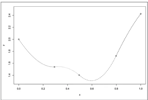
As an illustration, Figure 1 shows the results from a hypothetical PSA in which we plot the net benefit function, NBðx1;x2;x3Þ, against a single parameter of

interest,x1. The scatter of points suggests some kind

of U-shaped function. The dashed line shows a non-parametric regression of NBðx1;x2;x3Þ on x1. This

regression provides an estimate of the expected value EX2;X3jX15x1NBðx1;X2;X3Þas a function ofx1, that is,

it provides the gðd;xiÞ from Equation 8. In this

particular illustrative model, the expectation EX2;X3jX15x1NBðx1;X2;X3Þ can be obtained

analyti-cally (solid line), showing that the true expectation is very well estimated by the nonparametric regression.

Once we have obtained the regression function estimate,g^ðd;xÞ, for each decision option in our eco-nomic model, we can proceed to calculating the par-tial EVPI. Evaluating g^ðd;xÞat fx_ið1Þ;. . .;xð_iNÞg gives usfg^ðd;xð_i1ÞÞ;. . .;g^ðd;xð_iNÞÞg, which are the estimates of the conditional expectations that we require, and hence we can compute the partial EVPI by

d EVPIðXiÞ5

1

N XN

n51

max

d g^ðd;x ðnÞ i Þ max_d

1

N XN

n51

^ gðd;xðnÞ_i Þ:

ð9Þ

Note that we use maxd_N1PNn51g^ðd;x

ðnÞ

i Þ as our

Monte Carlo estimator of the second term in Equation 4 rather than maxd_N1PNn51NBðd;xðnÞÞ. By choosing

this as our estimator, we exploit the positive correla-tion between the 2 terms in Equacorrela-tion 9 and hence esti-mate the partial EVPI with increased precision.

We also note at this point that EVPI (calculated by any method) is invariant to the reexpression of net

benefits as incremental net benefits, relative to some chosen baseline option (which is therefore defined as having an absolute net benefit of zero). This reduces the number of regression problems fromDtoD1.

In the next sections, we give an overview of 2 partic-ular nonparametric regression methods that are suitable in this context, Gaussian process regression and regres-sion based on a Generalized Additive Model (GAM).

GAM Regression

When we adopt a GAM, we represent the unknown functiongðd;xiÞas the sum of a set of smooth functions

of the inputs. In the simplest form of GAM, we have

NBðd;xÞ5gðd;xiÞ1e;

gðd;xiÞ5s1ðx1Þ1. . .1spðxpÞ; ð10Þ where each smoothing functionsjðxjÞis a function of

one of the j51;. . .;p model input parameters of interest, and eis a mean-zero Normally distributed error with constant variance. For an introduction to GAM models, see Hastie and Tibshirani12or Wood.13 The usual choice for the smoothing functions is some form of spline, a common choice being the cubic spline. A cubic spline represents an arbitrary smooth function as a series of short cubic polyno-mials joined piecewise, as shown in Figure 2.

The cubic spline shown in Figure 2 can also be expressed as the weighted sum of a series of polyno-mial basis functions,blðxÞ, that take values ofxacross

the whole range ofx, rather than values in short seg-ments of the range ofx(this builds up the spline func-tion in a manner similar to the way in which an arbitrary sound wave can be built up from sine waves of increasing frequency). This allows us to write

y5sðxÞ5X L

l51

b_lblðxÞ; ð11Þ

for some basis dimensionL. The basis dimension con-trols the degree to which the spline can be ‘‘wiggly’’ (we can loosely think of this as akin to determining the number of segments in Figure 2). The basis functions themselves tend to be cumbersome to write out, and the reader is referred to Wood for further details.13

By expressing our unknown function (Equation 10) in the same way, we get

gðd;xiÞ5 XL1

l151

b_l1bl1ðx1Þ1. . .1 XLp

l51p

b_lpblpðxpÞ: ð12Þ

Estimation of the model coefficients is typically via penalized maximum likelihood, in which the penalties are designed to suppress overly wiggly esti-mates that would result in overfitting. The choice of basis dimension for each spline is usually not impor-tant as long as it is sufficiently large to avoid con-straining the spline to be overly inflexible (we found any any dimension greater than 3 to be suffi-cient). In practice, the software in which GAM is implemented makes the choice of basis dimension for each spline automatically.

Although the simple additive model in Equation 10 performs well in many situations, it will not ade-quately capture interactions between the input parameters of interest that may be a feature of the health economic model. To model interactions, we must include multivariate smoothing functions in our GAM model specification. So, for example, if we expect there to be interactions between inputsx1

andx2, then we would specify the model

gdðxiÞ5s1ðx1;x2Þ1s2ðx3Þ;. . .;sp1ðxpÞ: ð13Þ The multivariate smoothing functions1is built up

using a tensor product construction, which results in the spline’s being the sum of all multiplicative combi-nations of the basis functions for each variable,

s1ðx1;x2Þ5 XL1

l151 XL2

l251

b_l1l2bl1ðx1Þbl2ðx2Þ: ð14Þ

Modeling a large number of potential interactions does therefore have a cost. Given m inputs that are expected to interact in the economic model, and assuming the same basis dimension,n, for each input variable, the GAM model must estimate nm

coeffi-cients. Ifnm _{approaches the size of the PSA sample,}

then the GAM method will break down. This is one motivation for the more flexible Gaussian process regression approach described in the next section.

After estimating the GAM model parameters and hence obtaining g^ðd;xÞ, we can evaluate g^ðd;xÞ at the PSA inputs to givefgðd;xð_i1ÞÞ;. . .;gðd;xð_iNÞÞgand therefore the partial EVPI via Equation 9. The code in Box 1 illustrates the simplicity of the GAM regres-sion approach using the mgcv package in R.14In the example, there are 2 decision options, with the vector object INB holding the incremental net benefits from the PSA. The PSA samples from the 2 parameters of interest are held in vector objects x5 and x14. We assume the parameters do not interact in the model. If they did, we would simply replace the model for-mula INB ; s(x5)1s(x14) with the tensor product multivariate specification INB;te(x5,x14).

Box 1 Example R Code for Estimating Partial Expected Value of Perfect Information via

Generalized Additive Model Regression

library (mgcv)

model\- gam(INB ~ s(x5)1s(x14)) g.hat\- model$fitted

partial.evpi\ mean(pmax(0,g.hat)) -max(0,mean(g.hat))

A method for estimating the standard error of the GAM-based approximation of the partial EVPI is given in Appendix A. R functions for computing the partial EVPI via GAM and its standard error are avail-able at http://www.shef.ac.uk/scharr/sections/ph/ staff/profiles/mark.

Gaussian Process Regression

The Gaussian process is a highly flexible represen-tation of an unknown function, in our casegðd;xiÞ,

that again requires no parametric assumptions regarding functional form.15 When we model the function gðd;xiÞas a Gaussian process, we assume

that we can represent the unknown values of the function evaluated at the PSA inputs,

fgðd;xð_i1ÞÞ;. . .;gðd;xð_iNÞÞg, via a multivariate Normal distribution. To be more precise, we are representing our beliefs about the function using the multivariate Normal distribution. The function itself is unknown. We will therefore require a method for specifying the mean, variance, and covariance of the distribution that specifies our beliefs about the unknown function gðd;xiÞ given the PSA values fxð1Þ;. . .;xðNÞg and fNBðd;xð1Þ_{Þ;. . .;NBðd;x}ðNÞ_{Þgthat we have observed}

(sampled).

It is very important to note that by representing the unknown functiongðd;xiÞas a Gaussian process, we

do not require that the model input parametersxiare

Normally distributed (Gaussian) or that the net bene-fits NBðd;xÞ are Gaussian. In practice, the main requirement is thatgðd;xiÞ is a smooth function of

its inputs in the sense that for anyxð_inÞ andxð_imÞ that are close,gðd;xð_inÞÞandgðd;xð_imÞ) are also close. This is a weak requirement and likely to hold in most health economic models because costs and health benefits (e.g., quality-adjusted life-years [QALYs]) are usually continuous functions of the uncertain model input parameters.

Until now, the use of the Gaussian process in health economics has been rare and restricted to the modeling of the net benefit function in the context of a computationally expensive model.16–18 For a practical introduction to building Gaussian process models, see the Managing Uncertainty in Complex Models toolkit at mucm.aston.ac.uk/MUCM/MUCM-Toolkit/.

Gaussian Process Regression Model Specification. Recall that our PSA sample consists ofNinput vec-torsfxð1Þ_{;. . .;x}ðNÞ_{g and N corresponding net}

bene-fits fNBðd;xð1Þ_{Þ;. . .;NBðd;x}ðNÞ_{Þg for each decision}

option d. For each model run n51;. . .;N, we

have NBðd;xðnÞ_Þ5gðd;xðnÞ

i Þ1e

ðnÞ _{from Equation 8.}

We assume that the vector of unknown values of the functiongðd;xiÞevaluated at the PSA input

val-ues,fgðd;xð_i1ÞÞ;. . .;gðd;xð_iNÞÞg, jointly follows a mul-tivariate Normal distribution,

fgðd;x_ið1ÞÞ;. . .;gðd;xðNÞ_i Þg;NðHb;s2SÞ: ð15Þ The mean of the distribution Hb is a vector of lengthNand is the matrix product of a design matrix

H5

1 xð₁1Þ . . . xðp1Þ

1 xð₁2Þ . . . xðp2Þ .. . .. . .. . .. .

1 xðNÞ₁ . . . xðNÞp 0 B B B B @ 1 C C C C

A ð16Þ

of sizeN3q, (whereq5p11Þ, and a vector of regres-sorsb5ðb1;. . .;bqÞ. The covariance matrix is a

prod-uct of a scalar variance term s2 and a correlation matrixSof sizeN3N.

We require that the correlation matrixSdescribes the smoothness of the functiongðd;xiÞwith respect to

each input parameter of interest in the set ofpinputs that makes upxi. We therefore define thefn;mgth

ele-ment ofSto be a function of thepinput parameters of interest in the following way,

Sðn;mÞ5exp X

p

j51

fðxðnÞ_j xðmÞ_j Þ=djg 2

" #

: ð17Þ

The superscriptsðnÞandðmÞdenote arbitrary runs in the PSA sample, andjindexes thepparameters of interest that make up xi. The correlation length

hyperparameters dj describe the smoothness of

gðd;xiÞ with respect to each parameter of interest

and are estimated from the PSA sample as described below.

Note that the form of the correlation function ensures that diagonal entries in the matrixSare equal to 1 as they should be for a valid correlation matrix. To see why, observe that on the diagonal, we have

Sðn;nÞ5exp Pp_j51fðxð_jnÞxð_jnÞÞ=djg 2

h i

5expð0Þ51. The value of Sðn;mÞ, and therefore the correlation between gðxð_inÞÞ and gðxð_imÞÞ, decreases toward zero as the distance between xð_inÞ and xð_imÞ increases, with the values ofdjcontrolling how fast this decay

to zero occurs.

Finally, we require a method for learning aboutb,

s2_{, andd}

jfrom the net benefits, NBðd;xÞ. To do this,

we must link the Gaussian process model forgðd;xiÞ

net benefit obtained on the nth _{PSA model run,}

NBðd;xðnÞ_{Þ, is considered to be the sum of gðd;x}ðnÞ

i Þ

and a noise term eðnÞ_{, which implies that we can}

write

fNBðd;xð1Þ_Þ

;. . .;NBðd;xðNÞÞg;NfHb;s2ðS1nIÞg; ð18Þ where I is the identity matrix of sizeN and n is a ‘‘nugget’’ term that controls the variance of a Normally distributed mean zero, constant variance noise term e.19,20 For compactness of notation in the remainder of the article, we write S5S1nI and define the vectors nbd5fNBðd;xð1ÞÞ;. . .;NB ðd;xðNÞ_{Þg, g}

d5fgðd;x

ð1Þ

i Þ;. . .;gðd;x

ðNÞ

i Þg, and ^gd5 fg^ðd;xð_i1ÞÞ;. . .;g^ðd;xð_iNÞÞg.

Estimation of Hyperparameters b, s2, dj, and n.

The first step is to estimate the correlation lengths

dj and the nugget term nfrom the PSA sample. The

most straightforward approach is to find the values

b

dj and bn that maximize the joint posterior density

ofdj andngiven the net benefitsnbd. This requires numerical methods, and details are given in Appen-dix B. An R function is available at http://www.shef .ac.uk/scharr/sections/ph/staff/profiles/mark. Given

b

dj and bn (and hence S), the posterior mean of b,

which can be derived analytically, is

^

b5ðHTS1HÞ1HTS1nbd ð19Þ and the posterior mean ofs2is

b

s25ðnbdH

^

bÞTS1ðnbdHb^Þ

nq2 : ð20Þ

Estimation ofgðd;xiÞ.Once we have determinedS

andb^, we can use the properties of the Normal dis-tribution to obtain the expected value of g_d condi-tional on the net benefitsnbd,

^

gd5Hb^1SS 1

ðnbdHb^Þ: ð21Þ The components of g^d are fg^ðd;x

ð1Þ

i Þ;. . .;

^

gðd;xð_iNÞÞg and hence can be plugged into Equation 9 to give the partial EVPI. A method for estimating the standard error of the Gaussian process regression approximation for the partial EVPI is given in Appen-dix A. The R code for computing the Gaussian process regression-based partial EVPI and its standard error is available at http://www.shef.ac.uk/scharr/sections/ ph/staff/profiles/mark.

Implementation Issues and Regression Diagnostics

We recommended above that net benefits are expressed as incremental net benefits, relative to a chosen baseline option. This not only reduces the number of regression problems fromDtoD1but also improves numerical stability, particularly for the Gaussian process method. For the same reason, we also suggest that, for the Gaussian process method, the input parameters of interest are each scaled to lie in the ½0;1 interval. This ensures that the smoothness parametersdjare estimated on a

com-mon scale. EVPI is invariant to linear rescaling of the input parameters.

For both Gaussian process and GAM models, examination of the residuals is useful for assessing the robustness of assumptions. A plot of residuals (i.e.,y_d^gd) against fitted values (^gd) allows

assess-ment of the mean-variance relationship and will highlight deviation from the assumption of constant variance. A Normal quantile-quantile plot of resid-uals will show deviation from the assumption of Nor-mality of the residuals.

CASE STUDIES

Case Study 1: A Simple Decision Tree Model with Correlated Inputs

Case study 1 is based on a hypothetical decision tree model previously used for illustrative purpo-ses.5,7,9,10 The model predicts net benefit, NBðd;xÞ, under 2 decision options (d51;2) and can be written in sum product form as

NBð1;xÞ5lðx5x6x71x8x9x10Þ ðx11x2x3x4Þ; ð22Þ

NBð2;xÞ5lðx14x15x161x17x18x19Þ ðx111x12x13x4Þ;

ð23Þ

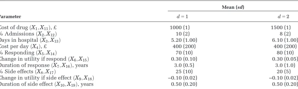
where x1;. . .;x19 are sampled realizations of the

uncertain input parameters X1;. . .;X19 listed in

Table 1, and the willingness to pay for 1 unit of health output in QALYs is l510;000=QALY. Note that some components of x5ðx1;. . .;x19Þare redundant

in NBðd;xÞfor eachd.

We assume that our uncertainty about the inputs can be represented by a multivariate Normal distribu-tion, withX5,X7,X14, andX16all pairwise correlated

with a correlation coefficient of 0.6, and withX6and

x15correlated with a correlation coefficient of 0.6. All

sum product form model, the assumption of multi-variate Normality allows us to compute the inner con-ditional expectation analytically.

We define 3 parameter sets of interest: set 1 com-prising effectiveness parameters X5 and X14,

repre-senting information that could be gained from a trial; set 2 comprising effectiveness and utility parametersX5;X6;X14andX15, representing

informa-tion that could be gained from a trial that also col-lected utility data; and set 3 comprising duration of response parametersX7andX16, representing

infor-mation that could be gained from the long-term fol-low-up of trial participants.

Although the case study model is computationally cheap to evaluate, we assume that we are in a position of being able to evaluate the model only 10 000 times. Given this limitation, we calculated partial EVPI using 3 methods. First, we calculated the partial EVPI for each parameter set using a single-loop Monte Carlo approximation for the outer expectation in the first term of the right-hand side of Equation 4 with 10 000 samples from the distribution of the parame-ters of interest, an analytic solution to the inner con-ditional expectation, and hence 10 000 model runs. Next, we calculated the partial EVPI values using the standard 2-level Monte Carlo approach with 3 dif-ferent sets ofJinner loop samples andK outer loop samples, where J3K = 10 000 model runs in total (see Table 2 for values ofJ andK). Third, we com-puted the partial EVPI values using the GAM regres-sion method with a total of 10 000 PSA samples. Finally, we computed the partial EVPI values using the Gaussian process regression method with the same 10 000 PSA samples.

We compared values with a gold standard measure of partial EVPI calculated using the analytic solution to the inner conditional expectation, and 107 outer

loop samples. Standard errors for the 2-level Monte Carlo partial EVPI estimates were obtained using the method given in Appendix A. Estimates of partial EVPI using the 2-level Monte Carlo method are upwardly biased for small values ofJ, due to the max-imization step. The estimates of upward bias were obtained using the method presented in Oakley and others9(see Appendix A).

For each method, we report the mean time taken to compute the partial EVPI for the 3 parameter sets of interest.

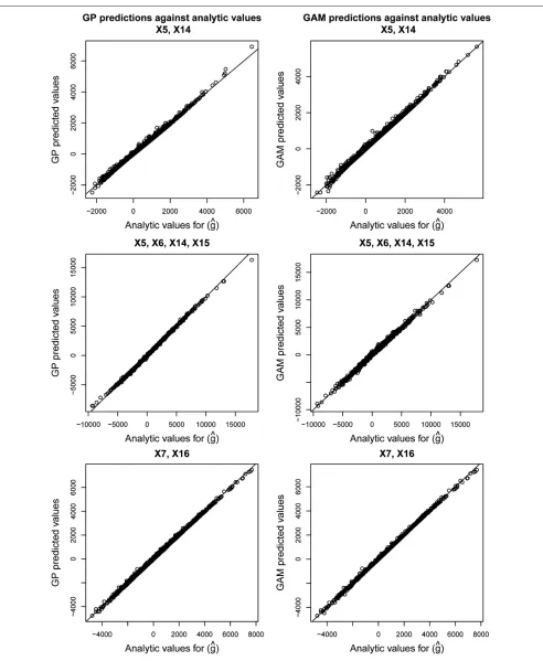
Results for Case Study 1. Regression diagnostic plots for the Gaussian process and GAM models are shown in Figure 3. A random subset of 500 points is shown on each plot. First of note is, for each parameter set, the similarity in the pattern of residuals between the Gaussian process model and the GAM model (reflecting the similarity in esti-mates of g). In each case, the plots of residuals against fitted values show no worrying heterosce-dasticity, and the residual Normal Q-Q plots show no gross deviation from Normality.

Figure 4 shows the values of g^ obtained via the regression methods against the analytically calcu-lated values of g. Good agreement is seen over the whole range.

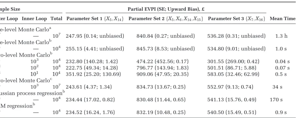
Table 2 shows the estimated partial EVPI values for the 3 sets of parameters of interest. The overall EVPI for all 19 parameters is £1047. The top line shows the gold standard estimates, obtained by generating 107samples from the joint distribution of the inputs of interest and then analytically calculating the expected net benefits for each decision option, condi-tional on these sampled values. The standard errors of the gold standard estimates are small. When we restrict ourselves to only 10 000 model evaluations,

Table 1 Summary of Means and Standard Deviations for Case Study Model Parameters

Mean (sd)

Parameter d51 d52

Cost of drugðX1;X11Þ, £ 1000 (1) 1500 (1)

% AdmissionsðX2;X12Þ 10 (2) 8 (2)

Days in hospitalðX3;X13Þ 5.20 (1.00) 6.10 (1.00)

Cost per dayðX4Þ, £ 400 (200) 400 (200)

% RespondingðX5;X14Þ 70 (10) 80 (10)

Change in utility if respondðX6;X15Þ 0.30 (0.10) 0.30 (0.05)

Duration of responseðX7;X16Þ, years 3.0 (0.5) 3.0 (1.0)

% Side effectsðX8;X17Þ 25 (10) 20 (5)

Change in utility if side effectðX9;X18Þ –0.10 (0.02) –0.10 (0.02)

but again use the analytic solution to the conditional expectation, the standard errors are unsurprisingly larger. The estimates are still unbiased. In contrast, estimates obtained via the 2-level Monte Carlo approach are biased due to the maximization over quantities that are subject to sampling variabil-ity.9When restricted to 10 000 model evaluations, there is a clear tradeoff between bias and variance when using the 2-level method, with small values of the inner loop resulting in considerable upward bias.

In comparison, the regression-based estimates all have lower variance than any of the 2-level Monte Carlo estimates when model runs are restricted to 10 000. The upward bias due to the max-imization in the first term of Equation 9 is small in each case and comparable with that obtained by the 2-level Monte Carlo method with 1000 inner loop samples. To achieve a similar level of bias and variance to that obtained using the regression method with 104 PSA samples, the 2-level Monte Carlo would require approximately 107 model runs.

The computational cost of obtaining the gold stan-dard estimate is greatest, because of the large sample size. The 2-level Monte Carlo method is fast in this example because of the simplicity of the model but will typically be slower and will increase as the com-putational complexity of the model increases. In con-trast, the speeds of the Gaussian process and GAM methods are independent of the computational

complexity of the model because the model itself is not evaluated during the regression fitting process. The GAM method takes less than 1 s with a PSA sam-ple size of 104, whereas the Gaussian process method takes approximately 3 min.

Case Study 2: Three State Markov Model

Case study 2 is an extension of the case study 1 model that incorporates a 20-time cycle Markov model for the response to each intervention. The parameters for mean duration of response (x7 and

x16) are replaced with Markov models of natural

his-tory of response to each drug with health states ‘‘responding,’’ ‘‘not responding,’’ and ‘‘dead.’’ The model is

NBð1;xÞ5l X

20

n51

ST₁Mn₁U1

1x8x9x10

( )

ðx11x2x3x4Þ;

ð24Þ

NBð2;xÞ5l X

20

n51

ST₂Mn₂U2

1x17x18x19

( )

ðx111x12x13x4Þ;

ð25Þ

where the vectors Sd and Ud are defined as

S15ðx5;1x5;0ÞT, S25ðx14;1x14;0ÞT, U15ðx6;

0;0ÞT, and U25ðx15;0;0ÞTand where the transition

matrices are defined as

Table 2 Partial Expected Value of Perfect Information (EVPI) Values and Timings for Case Study 1

Sample Size Partial EVPI (SE; Upward Bias), £

Outer Loop Inner Loop Total Parameter Set 1fX5;X14g Parameter Set 2fX5;X6;X14;X15g Parameter Set 3fX7;X16g Mean Time

One-level Monte Carloa

107 — 107 247.95 (0.14; unbiased) 840.84 (0.27; unbiased) 536.28 (0.31; unbiased) 1.3 h One-level Monte Carlob

104 — 104 255.15 (4.41; unbiased) 845.73 (8.53; unbiased) 534.80 (9.01; unbiased) 1.0 s Two-level Monte Carlob

101 ₁₀3 ₁₀4 _{232.80 (140.28; 1.42) 474.22 (452.56; 0.17) 301.55 (269.00; 0.42) 0.04 s}

102 102 104 222.75 (49.34; 14.28) 796.77 (143.94; 1.83) 501.51 (86.71; 5.88) 0.07 s 103 ₁₀1 ₁₀4 _{351.92 (25.20; 130.69) 909.06 (47.95; 20.35) 583.05 (32.46; 62.99) 0.5 s}

Two-level Monte Carloc

104 ₁₀3 ₁₀7 _{243.61 (4.37; 1.34) 834.73 (13.67; 0.25) 552.97 (9.13; 0.74) 34 s}

Gaussian process regressionb

104 — 104 234.44 (17.02, 0.82) 830.48 (11.44, 0.65) 541.13 (15.76, 0.49) 170 s GAM regressionb

104 — 104 234.52 (16.24, 1.76) 832.19 (10.48, 0.25) 540.50 (15.49, 0.51) 0.9 s

a. Reference gold standard. b. Model runs restricted to 104_.

M15

x20 x21 x22 x23 x24 x25

0 0 1

0 @

1

AandM25

x26 x27 x28 x29 x30 x31

0 0 1

0 @

1 A: ð26Þ

Uncertainty regarding the transition matrix param-eters (X20toX31) was expressed using Dirichlet

distri-butions with ðX20;X21;X22Þ; Dirichlet(70,40,10); ðX23;X24;X25Þ; Dirichlet(10,100,20); ðX26;X27;

X28Þ; Dirichlet(70,40,10); and ðX29;X30;X31Þ;

Dirichlet(10,100,20). Means and standard deviations for the remaining input parameters are as for case study 1 (Table 1), but now instead of assuming Nor-mality for all parameters, we expressed our uncer-tainty about X2;X5;X8;X12;X14 and X17 using Beta

distributions and our uncertainty about X3;X4;X10;X13 and X19 using Gamma distributions.

In contrast with case study 1, it is assumed that each input parameterX1toX19is independent of all

other parameters in the model.

We again defined 3 parameter sets of interest: set 1 comprising effectiveness parameters X5 and X14,

representing information that could be gained from a trial; set 2 comprising effectiveness and utility parametersX5;X6;X14andX15, representing

informa-tion that could be gained from a trial that also col-lected utility data; and set 3 comprising the transition matrix parametersX20toX31, representing

information that could be gained from the long-term follow-up of trial participants.

Results for Case Study 2. A similar pattern of results is seen for case study 2 as for case study 1.

Regression diagnostic plots shown in Figure 5 are similar in character to the those obtained in the first case study, and again, no worrying departures from the model assumptions are indicated.

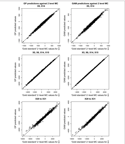
Figure 6 shows the values ofg^ calculated by the regression methods against the corresponding values obtained by the 2-level Monte Carlo method with 108 model runs (defined as our gold standard in this case). Very good agreement is seen over the whole range ofgin each case.

Table 3 shows the estimated partial EVPI values. The overall EVPI is £775. Standard errors for the gold standard 2-level Monte Carlo estimates with 108 model runs are small, as are the values of the upward bias. When the number of model evaluations is restricted to 104, the regression methods perform considerably better than the 2-level Monte Carlo method, resulting in estimates that have both mini-mal upward bias and substantially greater precision. To achieve a similar level of bias and variance to that obtained using the regression method with 104PSA samples, the 2-level Monte Carlo would require approximately 107model runs.

With a PSA sample size of 104, the GAM takes approximately 1 s and the Gaussian process takes approximately 3 min. In contrast, the 2-level Monte Carlo method with 107model runs takes 1.8 h.

DISCUSSION

Main Result and Implications

The regression-based approach we propose requires only the single set of model evaluations that is generated in a standard probabilistic sensitiv-ity analysis to calculate partial EVPI for any set of inputs. It leads to a considerable gain in precision over the 2-level Monte Carlo method with the same number of model runs while retaining an acceptably small upward bias. The GAM method in particular is straightforward to implement in the freely available software R, thus allowing an analyst to compute par-tial EVPI for any subset of input parameters quickly and with relative ease.

The regression method allows the complete sepa-ration of the EVPI calculation step from the model evaluation step, which may be particularly useful when the model has been built using specialist soft-ware (e.g., for discrete event simulation) that does not allow easy implementation of the EVPI step or where those who wish to compute the EVPI do not own (and therefore cannot directly evaluate) the

model. The method has the particular advantage that, even in the case of correlated inputs, only the joint distribution of inputs is required. This is in con-trast to the 2-level Monte Carlo approach in which we are required to sample values frompðXijXi5xiÞ, the

conditional distribution of the remaining parameters given some sampled parameter vector of interest, a process that an analyst could find challenging with-out the necessary statistical training.

In terms of computational speed, the regression methods are fast. We see 2 particular scenarios in which this will be useful: when the analyst is faced with a slow patient-level simulation model and in the case in which the partial EVPI calculation would require computationally demanding MCMC sam-pling under the 2-level scheme.

For health economic decision analysts, the key implication of the nonparametric regression approach is that the computation of partial EVPI has become tractable for any decision problem. We hope that the computation of partial EVPI values now becomes standard practice, and we urge those who write guidance on good modeling practice to promote the routine reporting of EVPI values.

Limitations

There are some limitations of the regression approaches. In general, the GAM method will be more straightforward to implement because of the easy availability of software (e.g., the mgcv package in R). However, if the set of input parameters for which we wish to calculate partial EVPI is moderately large (greater than 6 or so), and if it is expected that those parameters will jointly interact (nonadditively) within the economic model, then it is likely that the number of GAM model parameters that need to be estimated will exceed the number of data points, causing the method to fail. In this case, we would recommend using the Gaussian process approach.

places a practical limit on the size ofN(currently of the order of tens of thousands), which in turn limits the precision that can be achieved with the Gaussian process method. Finally, the use of the Gaussian pro-cess currently requires somewhat more work on the part of the analyst than the GAM approach, even with the functions that we have made available.

Using the Method in Patient-Level Models

In our introduction, we presented a typical sce-nario in which obtaining partial EVPI via 2-level Monte Carlo was likely to be computationally prohib-itive due to the requirement to sample many thou-sands of patients within each evaluation of the inner loop.

Partial EVPI via the regression method is calcu-lated for a patient-level model in the same manner as it is for a cohort model (i.e., by regressing the PSA sample net benefits on the parameters of inter-est). We briefly recap here the computation of a PSA for a patient-level model. This is a 2-level process whereby samples are drawn from the PSA level (i.e., population level) parameters in an outer loop, and then, conditional on these samples, individual patients are sampled in an inner loop. The purpose of sampling individual patients is to average over het-erogeneity (and/or uncertainty) at the patient level for each sample of population-level input parameters. Convergence is achieved when the patient-level sam-ple size is large enough that, given some arbitrary sample from the PSA (population)–level parameters,

the estimated net benefit is stable. Nonconvergence will introduce additional noise in the estimation of the net benefit for each sample from the PSAlevel parameters.

Now, recall that in our approach, we treat all vari-ability in the net benefit that is not due to the param-eters of interest as noise (Equation 8). Any residual variability due to nonconvergence of the patient-level simulation will be treated as noise in the regression and averaged out. Because the regression estimation occurs before the maximization step, the residual first-order uncertainty will not cause an upward bias in the partial EVPI estimate.

Other Uses of the Gaussian Process in Health Economic Decision Modeling

In our method, we modeled the target conditional net benefit as an unknown smooth function of the parameters of interest. The observed net benefits in the PSA sample were treated as noisy data from which to learn about the unknown function. This use of a nonparametric regression method to approx-imate the (conditional) output of a health economic decision model is subtly different from the use of the Gaussian process in previous work by Stevenson and others,16 Tappenden and others,17 and Rojnik and Naversnik.18In these previous applications, the Gaussian process was used to model the net benefit itself as an unknown function of all the unknown input parameters, rather than to model the

conditional net benefit as a function of the parameters of interest only. The primary purpose for using the Gaussian process was to construct a meta-model or emulator for the health economic decision model to allow a slow model to be replaced by a fast surrogate. Although this approach reduces computation time, the calculation of partial EVPI will typically still require a nested 2-level Monte Carlo approach. More importantly, this use of the Gaussian process does not address the problem of sampling from poten-tially difficult conditional distributions if input parameters are correlated.

Further Research

Although partial EVPI is useful in highlighting the sensitivity of the decision to any particular subset of input parameters, it represents only an upper bound on the expected value of undertaking research to reduce decision uncertainty. More useful is the expected value of sample information (EVSI), which represents the expected value of undertaking a partic-ular data collection exercise.11 We are currently working on extending the regression method described above to the computation of EVSI.

Conclusion

In conclusion, the regression-based approach to computing partial EVPI is likely to be of considerable benefit over the traditional 2-level Monte Carlo approach, except perhaps in models that are

Table 3 Partial Expected Value of Perfect Information (EVPI) Values and Timings for Case Study 2

Sample Size Partial EVPI (SE; upward bias), £

Mean Time Outer Loop

Inner

Loop Total

Parameter Set 1fX5;X14g

Parameter Set 2fX5;X6;X14;X15g

Parameter Set 3fX20toX31g

Two-level Monte Carloa

104 104 108 67.95 (1.43; 0.22) 587.14 (9.38; 0.03) 416.80 (6.50; 0.05) 17.7 h Two-level Monte Carlob

101 ₁₀3 ₁₀4 _{5.77 (50.66; 2.01) 389.93 (296.6; 0.29) 178.93 (223.02; 0.39) 3.7 s}

102 102 104 77.07 (21.96; 19.98) 661.75 (94.34; 2.40) 362.82 (71.78; 4.41) 2.9 s 103 101 104 228.32 (15.11; 148.24) 623.70 (31.43; 21.63) 467.61 (26.06; 42.32) 2.8 s Two-level Monte Carloc

104 103 107 68.84 (4.47; 0.22) 595.14 (9.39; 0.13) 426.67 (6.51; 0.30) 1.8 h GP regressionb

104 _{— 10}4 _{62.36 (10.35; 0.64) 582.32 (8.85; 0.13) 408.17 (10.30; 2.01) 198 s}

GAM regressionb

104 — 104 62.53 (9.98; 0.47) 582.03 (8.23; 0.49) 409.80 (10.37; 1.03) 0.9 s

a. Reference gold standard. b. Model runs restricted to 104_.

computationally very cheap to evaluate and in which there are no correlations in the inputs. With the increasing use of patient-level micro-simulation models, we envisage that obtaining partial EVPI via the traditional 2-level Monte Carlo approach will be considered just too time-consuming (in fact, experi-ence suggests that the 2-level Monte Carlo procedure is considered too difficult for even moderately simple cohort models). In contrast, the regression methods we have presented provide a mechanism for rapidly estimating partial EVPI for any set of parameters in a model of any complexity.

REFERENCES

1. Raiffa H. Decision Analysis: Introductory Lectures on Choices Under Uncertainty. Reading, MA: Addison-Wesley; 1968. 2. Claxton K, Posnett J. An economic approach to clinical trial design and research priority-setting. Health Econ. 1996;5(6): 513–24.

3. Felli JC, Hazen GB. Sensitivity analysis and the expected value of perfect information. Med Decis Making. 1998;18(1):95–109. 4. Felli JC, Hazen GB. Erratum: Correction: sensitivity analysis and the expected value of perfect information. Med Decis Making. 2003;23(1):97.

5. Brennan A, Kharroubi S, O’Hagan A, Chilcott J. Calculating par-tial expected value of perfect information via Monte Carlo sam-pling algorithms. Med Decis Making. 2007;27(4):448–70. 6. Koerkamp BG, Myriam Hunink MG, Stijnen T, Weinstein MC. Identifying key parameters in cost-effectiveness analysis using value of information: a comparison of methods. Health Econ. 2006;15(4):383–92.

7. Strong M, Oakley JE. An efficient method for computing single-parameter partial expected value of perfect information. Med Decis Making. 2012;33(6):755–66.

8. Sadatsafavi M, Bansback N, Zafari Z, Najafzadeh M, Marra C. Need for speed: an efficient algorithm for calculation of

single-parameter expected value of partial perfect information. Value Health. 2013;16(2):438–48.

9. Oakley JE, Brennan A, Tappenden P, Chilcott J. Simulation sam-ple sizes for Monte Carlo partial EVPI calculations. J Health Econ. 2010;29(3):468–77.

10. Kharroubi SA, Brennan A, Strong M. Estimating expected value of sample information for incomplete data models using Bayesian approximation. Med Decis Making. 2011;31(6):839–52. 11. Ades AE, Lu G, Claxton K. Expected value of sample informa-tion calculainforma-tions in medical decision modeling. Med Decis Mak-ing. 2004;24(2):207–27.

12. Hastie T, Tibshirani R. Generalized additive models. Stat Sci. 1986;1(3):297–318.

13. Wood SN. Generalized Additive Models: An Introduction with R. Boca Raton, FL: Chapman and Hall/CRC; 2006.

14. R Development Core Team. R: A Language and Environment for Statistical Computing. Vienna, Austria; 2012. Available from: URL: http://www.R-project.org/

15. Rasmussen CE, Williams CKI. Gaussian Processes for Machine Learning. Cambridge, MA: MIT Press; 2006.

16. Stevenson MD, Oakley J, Chilcott JB. Gaussian process model-ing in conjunction with individual patient simulation modelmodel-ing: a case study describing the calculation of cost-effectiveness ratios for the treatment of established osteoporosis. Med Decis Making. 2004;24(1):89–100.

17. Tappenden P, Chilcott JB, Eggington S, Oakley J, McCabe C. Methods for expected value of information analysis in complex health economic models: developments on the health economics of interferon-beta and glatiramer acetate for multiple sclerosis. Health Technol Assess. 2004;8(27):1–78.

18. Rojnik K, Naversnik K. Gaussian process metamodeling in Bayesian value of information analysis: a case of the complex health economic model for breast cancer screening. Value Health. 2008;11(2):240–50.

19. Andrianakis I, Challenor PG. The effect of the nugget on Gauss-ian process emulators of computer models. Comput Stat Data Anal. 2012;56(12):4215–28.