Automatic feature detection and interpretation in borehole data

(1)

Automatic Feature Detection and Interpretation

in Borehole Data

Thesis submitted in accordance with the requirements of

the University of Liverpool for the degree of Doctor in Philosophy

by

Waleed Tayseer Al-Sit

June 2015

c

(2)

Abstract

Detailed characterisation of the structure of subsurface fractures is greatly facilitated by digital borehole logging instruments, however, the interpretation of which is typi-cally time-consuming and labour-intensive. Despite recent advances towards autonomy and automation, the final interpretation remains heavily dependent on the skill, expe-rience, alertness and consistency of a human operator. Existing computational tools fail to detect layers between rocks that do not exhibit distinct fracture boundaries, and often struggle characterising cross-cutting layers and partial fractures. This research proposes a novel approach to the characterisation of planar rock discontinuities from digital images of borehole logs by using visual texture segmentation and pattern recog-nition techniques with an iterative adaptation of the Hough transform. This approach has successfully detected non-distinct, partial, distorted and steep fractures and layers in a fully automated fashion and at a relatively low computational cost.

Borehole geometry or breakouts (e.g.borehole wall elongation or compression) and imaging tool decentralisation problem affect fracture characterisation and the quality of extracted geological parameters. This research presents a novel approach to the char-acterisation of distorted fracture in deformed borehole geometry by using least square ellipse fitting and modified Hough transform. This approach approach has successfully detected distorted fractures in deformed borehole geometry using simulated data.

To increase the fracture detection accuracy, this research uses multi-sensor data combination by combining extracted edges from different borehole data. This approach has successfully increased true positive detection rate.

(3)

To my

Dear father and mother

Lovely wife and son

Great brother

and

(4)

Acknowledgement

Foremost, I owe my sincere and earnest appreciation to my supervisor Dr. Waleed

Al-Nuaimy for the continuous support of my Ph.D study and research, for his

pa-tience, motivation, enthusiasm, and immense knowledge throughout the course

of this work.

Special thanks and appreciation are also extended to all members of my family

for their encouragement and patience, and to anyone who supported me during

the work in this project.

I also express my warmest gratitude to Mu’tah University and Ministry of

Higher Education and Scientific Research, The Hashemite Kingdom of Jordan

for their generous financial support. My thanks extend to Roberson Geologging

(5)

List of Figures

1.1 Borehole top view [1] . . . 2

1.2 Graphical representation of stress-induced borehole breakout [2] . 4 1.3 Illustration showing a planar feature intersecting a borehole and its typical sinusoidal appearance in the unwrapped presentation. (N, E, S, W) are the four directions . . . 5

1.4 Block diagram of the proposed fracture detection method . . . 10

2.1 Optical televiewer probe [3] . . . 16

2.2 Optical televiewer borehole logs sample . . . 17

2.3 Acoustic borehole log [4] . . . 18

2.4 Illustration of acoustic acquisition tool [4] . . . 19

2.5 Resistivity log sample . . . 21

2.6 Contrast-enhancement caused by background removal . . . 23

2.7 Probe decentralisation cases . . . 25

3.1 Processing stages of texture segmentation system . . . 29

3.2 Example of the reflected image border to overcome the difficulty in computing boundary features . . . 34

3.3 Formation of feature vector from feature images . . . 38

3.4 Stages of multi-resolution texture segmentation procedure . . . . 40

3.5 Graphical illustration of the effect of filter frequency (u0), space

(9)

3.6 Plot of MH index versus number of categories showing significant

knee at four classes in Figure 2.2 . . . 49

3.7 Patches selected from borehole image, representative of different visual textures . . . 50

3.8 Four-quadrants image of representative categories . . . 50

3.9 Simple Kohonen competitive learning network [6] . . . 51

3.10 Illustration of winner-take-all weight update [6] . . . 53

3.11 Results of four-quadrant image in Figure 3.8 . . . 54

3.12 Image segmentation . . . 55

3.13 Comparison of the segmentation results using statistical and multi-channel texture features . . . 58

4.1 (a) Segmented image (b) Edge detection result using modified Canny edge detection . . . 63

4.2 (a) Detected edge, (b) Edges after custom skeletonisation . . . 64

4.3 Hough transform accumulator . . . 67

4.4 (a) Multiple layers of volcanic rock not exhibiting visible fractures, (b) Poorly-defined rock layers correctly delineated . . . 70

4.5 (a) Cross-cutting and partial fractures Optical, (b) Cross-cutting and partial fractures detected automatically . . . 71

4.6 (a) High angle fracture, (b) High angle and disjointed fractures characterised . . . 72

4.7 (a) Acoustic borehole image- Amplitude data, (b) Detection result 73 4.8 (a) Resistivity borehole image (b) Detection result . . . 74

(10)

5.3 Example 1: Borehole shape and its fracture shape. The black line

represents distorted borehole while the red line represents in-gauge

borehole . . . 82

5.4 Example 2: Borehole shape and its fracture shape. The black line represents distorted borehole, while the red line represents in-gauge borehole . . . 83

5.5 Fracture detection results in different borehole geometries. The black line represents detected fracture using proposed method, while the red line represents detected fracture using conventional Hough transform . . . 84

5.6 Edge detection in acoustic amplitude borehole data . . . 88

5.7 Edge detection in optical borehole data . . . 89

5.8 Combined extracted edges of optical and acoustic borehole data . 89 5.9 Comparison of fracture detection between using data fusion and single borehole data . . . 90

A.1 Acoustic borehole data detection result . . . 109

A.2 Resistivity borehole data detection result . . . 111

C.1 GUI tool main menu . . . 117

C.2 Edge detection processing window . . . 118

C.3 Synthetic result window . . . 118

(11)

Chapter 1 Introduction

1.1 Background

Borehole imaging enables geophysicists to characterise subsurface conditions in

considerable detail, detailing lithologic and groundwater flow conditions and

iden-tifying fractures, faults, layers and veins within the subsurface rock strata,

facili-tating the characterisation of intrusions for mining and geotechnical assessments.

Such subsurface surveys require multi-sensor logging instrumentation to measure

the fracture and bedding-plane dip and dip angle [9].

Borehole imaging tools provide an image for the borehole wall based on

phys-ical property contrast for the rock as shown in Figure 1.1. Nowadays, there is a

wide range of imaging tools, these fall into three categories: optical, acoustic and

resistivity. In mining geology, image logs are digital images acquired by a

log-ging tool within a borehole. They represent measurements of the rock formation

taken to the wellbore surface. Borehole imaging provides a high resolution images

of borehole wall that contain information about layer properties, fractures and

sedimentary structures. Interpretation of borehole data provides geologists with

(12)

[image:12.612.148.493.71.299.2]

Figure 1.1: Borehole top view [1]

i.e, exploration for oil and gas, water mining.

Data processing is intensively performed after each logging acquisition, even

integrating information from other tools, to characterise the features in terms of

type, shape, dip and dip direction. This process is usually done manually by the

experts, and it is an intensely time consuming task, depending heavily on the

skill, experience, alertness and consistency of the operator, and the

interpreta-tion of the large volumes of borehole data are extremely challenging and often

presents as implementation bottleneck.

The recent methods that have been developed to facilitate data interpretation

typically involve mathematical model or image processing resulting in an

awk-ward and computational intensive system inapplicable for online processing and

large volume of data.

This research proposes algorithms to automatically detect and characterise

(13)

(optical, ultrasonic and resistivity). In order to achieve this, a number of novel

data manipulation and processing methods have been deployed to extract

infor-mation from different logs type, and several visual texture approaches employing

the wavelet and texture analysis have been used for fracture detection. In

addi-tion, it proposes algorithms to detect, characterise and correct a distorted fracture

in non-circular borehole shape.

1.2 Borehole Fractures

Breakout theory was originally proposed by Bell [10] and Gough [7], based on

the equations in [11, 12]. The borehole breakout method is an important

indica-tor of horizontal stress orientation, particularly in seismic regions and at small

and intermediate depths. Borehole breakouts are stress-induced elongations that

commonly appear over large sections along a borehole. As a result, borehole

breakouts may provide continuous information on the state of stress, and

there-fore reveal important information on the continuity of the stress field in the rock

mass [13]. Borehole breakouts can be detected using standard geophysical logging

tools that map the geometry of the borehole wall.

Borehole fractures are stress caused by the enlargements of the borehole

cross-section [14,15]. When the material are removed form the subsurface after borehole

drilling, it is no longer supporting the surrounding rock, this causes the stress

be-come concentrated around borehole wall as shown in Figure 1.2, where σH and σh are the maximum and minimum horizontal stresses. Borehole fractures

hap-pen when the stresses around borehole exceed that required to cause compressive

failure of the borehole wall [16, 17].

(14)

[image:14.612.150.485.73.363.2]

Figure 1.2: Graphical representation of stress-induced borehole breakout [2]

from geophysical point of view, it can help geologists to understand the stress

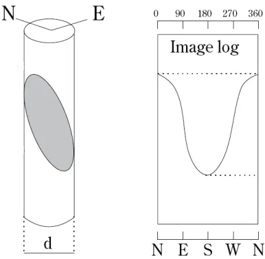
sit-uation around borehole wall and borehole stability. Fractures appear as sinusoids

assuming the borehole to be cylindrical and are cutting by a planar fracture, as

a result, the unwrapping image will show sinusoid as shown in Figure 1.3.

With reference to Figure 1.3, the dip direction with a cylindrical borehole is

defined as the direction of the line formed by the intersection of a planar feature

and a horizontal plane, while the dip angle gives the steepest angle of descent of

a tilted bed or feature relative to a horizontal plane:

dip angle = arctan( ˆA/r) (1.1)

(15)

ra-Figure 1.3: Illustration showing a planar feature intersecting a borehole and its typical sinusoidal appearance in the unwrapped presentation. (N, E, S, W) are

the four directions

dius [18].

Borehole stability is weighted by fracture density (number of fractures in the

well per unit well length). Failure in detecting the fracture correctly leads to [19]:

(i) increases the risk of drilling through fractured rock.

(ii) increases the probability of borehole collapse.

1.3 Previous Work

The standard approach for automated geological feature detection, i.e. computing

an edge map and searching for sinusoids, has been widely applied in commercial

borehole processing software. Thapa et al [18] proposed a semi-automated

bore-hole log interpretation system based on the Hough transform. A 3D accumulator

was constructed in parameter space to find the amplitude, phase and offset. The

edge pixel candidates were selected according to the assumption that the

[image:15.612.226.419.72.261.2]

(16)

of this method is the time consumption and the amount of memory needed for

the three dimensional Hough transform to find the amplitude, phase and offset of

sinusoidal waves. Taking the darkest 10% of the pixels to be geological features

excludes a large category of geological features and this is a limitation. Glossop

et al [20] used an algorithm similar to that by Thapa [18], the difference lies in

the highlighting, which Glossop does using a Laplace-of-Gaussian filter.

Changchun [21] suggests an approach to reduce the complexity of Hough

trans-form and decompose the problem of finding sinusoidal waves from 3D into 2D,

thus reducing computational time and storage space. His algorithm is based

on searching the midpoint that matched every pair of points in a fixed period.

However, no experiments were conducted on real borehole images to verify this

method.

Malone et al [22] proposed a system called the Borehole and Ice Feature

An-notation (BIFA), providing the users with automatic or manual glacier borehole

image annotation options. The automatic annotation algorithm is based on a

modified version of the Canny edge detector to find edges based on intensity

changes in the image; the user has the ability to customise Canny edge

param-eters, and after edges have been detected, the method of least squares is used

to fit sinusoids onto edges in borehole images. For manual detection, the user

has to select the highest and the lowest point of the edge, and the sinusoid is

automatically detected.

He and Wang [23] proposed a method for rock fracture detection only using

edge detection based on pulse coupled neural network (PCNN). The method was

compared with well-known edge detection methods such as Canny edge detection

(17)

false edges but still contains noise and was only applied to one example, and the

detected fractures were not characterised.

Wanget al [24] proposed a method based on edge detection and support

vec-tor machines (SVM). The proposed method is based on the concept of region

detection using Canny edge detection to obtain a segmented image, then from

the segmented image, 11 geometrical and statistical parameters were extracted

to form the input vector to the classifier. The authors acknowledged that the

proposed method did not achieve a good performance and without fracture

char-acterisation results.

Johansson [25] proposed a method to extract and characterise fractures. The

method is based on iterative intensity thresholding by extracting the darkest

pix-els in the image then the immediate neighbour pixpix-els are included, this process is

repeated until the fracture trace is filled. The fitting process is made as a method

of least square fitting (LSF). The results showed that this method traces some

fractures successfully but without fracture characterization results.

Ginkel et al [26] used a 3D generalised Radon transform to transform edge

map into parameter space followed by post-processing to reduce the amount of

incorrect picks by recomputing the Radon integral at all local maxima in

param-eter space and erase all points that support the curve from the orientation space.

Their method was applied to resistivity borehole data and the authors

acknowl-edged that the performance is at the expense of a considerable computational

burden.

Assous et al [27] proposed a method to extract and characterise fractures in

(18)

de-tection and phase congruency implemented using Log Gabor wavelets to validate

detected edges followed by sinusoid detection and 2D accumulator for sinusoid

estimation. The authors claimed a false positive rate between 2% and 5% for

resistivity data, with a computationally-efficient algorithm.

The borehole images suffer from a number of distortions, most of which can

be identified as follows:

(a) Imperfect sinusoids due to:

(i) Variations in the speed of the tool.

(ii) The borehole is not perfectly cylindrical.

(iii) The fracture is not perfectly planar.

(b) Partial sinusoids due to:

(i) Missing data due to the partial coverage.

(ii) True partial fractures (either through cementation or drilling induced

fractures).

(c) Structures other than fractures introduced by some of the effects above,

especially the partial coverage and the speed variations.

Most published experiments have been performed in boreholes with very well

defined features and low levels of noise, which are not always representative of real

geological data when related, for example, to complex depositional environment

and field of stress or even dealing with rough borehole walls, impurities in the

fluid or drilling-induced scratches. The existing algorithms are generally unable

(19)

Fracture shape and parameters are directly related to the actual borehole

geometries, it appears as an ideal sinusoid if it is assumed that the borehole is

cylindrical and is cutting by a planar fracture. However, when the imaging tool

is decentralised, or the borehole wall is elongated or compressed, the fracture

ap-pears as a distorted sinusoid, and provides non-meaningful geological parameters

(i.e. dip and dip direction). Knowing the borehole geometry and dimensions will

help to detect the fractures accurately.

In order to overcome the limitations of the current borehole image

interpre-tation and annointerpre-tation systems, a new scheme for geological features detection

in borehole images based on multi-resolution texture segmentation and pattern

recognition techniques is proposed to reduce human interaction with the

inter-pretation process so as to be fully automated. The combination of visual texture

segmentation and iterative use of the modified 2D Hough transform results in

reducing the false peak detection, as well as enhancing the overall method

ac-curacy. Enhancing automated detection accuracy reduces human involvement in

the final result. The proposed method provides a non-subjective and accurate

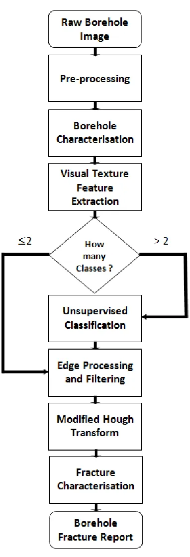
computer-based detection system for eminent borehole fractures. The block

dia-gram of the proposed method is summarised in Figure 1.4.

The proposed method consists of the following steps:

(i) Borehole data is pre-processed in order to remove noise and clutters

(ii) Borehole characterisation using travel-time acoustic data.

(iii) Features extraction based on visual texture.

(iv) Modified Hubert (MH) index for number of cluster determination.

(20)

[image:20.612.221.412.106.666.2]

(21)

(vi) Edge detection based on modified Canny edge detection.

(vii) Fracture detection and characterisation using modified Hough Transform(HT).

Moreover, to solve the problem of detecting distorted fracture shape form

decentralised borehole data or breakout borehole, a new method based on

non-linear least squares ellipse fitting to find the actual borehole geometry is proposed,

followed by a modified version of Hough transform to detect and characterise

the distorted fracture in deformed borehole. The proposed method successfully

obtains accurate fracture parameters from non-circular borehole shape.

1.4 Aims and Research Objectives

This study addresses some of the issues outlined above, by adopting and

devel-oping a range of signal and image processing techniques from other disciplines

into a comprehensive automated geological features that can be used effectively

by untrained operator. The goal is to develop and apply the techniques necessary

to provide automated borehole interpretation report without the requirement for

extensive processing by the human operator. The particular anomaly types that

this research is considering are:

(i) Rock layers that separated two different rock types.

(ii) Fractures and cross-layer that represent faults and breaks in the borehole

wall.

The completed system processes different borehole log types, i.e; optical,

acoustic and resistivity, to detect and characterise geological features

indicat-ing its dip and direction information. This information is required to be accurate

and prompt. The requirements need a high degree of automation, and robustness

(22)

1.5 Thesis Structure

This thesis is structured as follows: Chapter 2 describes the operation of various

types of borehole imaging system and the data acquisition process and the

pre-processing stages that prepare data for interpretation. Chapter 3 presents visual

textures analysis to discriminate the geological features, while Chapter 4 presents

edge detection techniques and fractures characterisation. Chapter 5 presents

distorted fracture detection in deformed borehole shape, and multi-sensor data

combination techniques that used to aggregate different borehole logs in order to

enhance the overall system detection accuracy. Chapter 6 concludes the research

by highlighting the achievements made to meet the objectives, pointing out the

shortcomings and discussing the future research.

1.6 Contribution

The main contributions of the research work described in this thesis are:

(i) Proposed method to detect and characterise non-distinct, cross-cutting,

partial fractures, high angle and disjointed fractures and layers from

dif-ferent types of borehole data, based on visual texture segmentation. The

method proves to be accurate and non-subjective.

(ii) Proposed method for borehole shape modelling and automatic distorted

fracture detection in deformed borehole geometry using acoustic borehole

data. The proposed method is based on non-linear ellipse fitting and

adap-tive Hough transform, and detects distorted fracture shape and parameters

(23)

(iii) Proposed method for fracture detection result enhancement by using

multi-sensor data combination techniques.

1.7 Published Work

W. Al-Sit, W. Al-Nuaimy, M. Marelli, and A. Al-Ataby, ”Visual texture for

automated characterisation of geological features in borehole televiewer imagery,”

(24)

Chapter 2 Data Acquisition and

Pre-Processing

2.1 Introduction

Borehole scanner tools which measure physical properties in different directions

in a borehole allow to derive the directional dependence of rock properties in the

case of anisotropic formations (e.g., crystals, cracks, pores, layers or inclusions).

Among the scanner tools, borehole image tools produce images of the borehole

wall which are influenced by the surface of the borehole wall or a very small

depth of penetration of only a few millimetres. One fascinating aspect of these

image tools is that the data obtained can be presented on a computer like a core.

Then, it is possible to display and interpret on screen these virtual core images

with the associated virtual optical images of real cores created by an optical core

scanner [28].

Borehole Imaging tools provide an image for the borehole wall based on

phys-ical property contrast for the rock. Nowadays, there are a wide range of imaging

(25)

illustration of each method will be presented in the next sections. All

meth-ods utilise a built-in flux-gate magnetometer to orient the image with respect to

magnetic north. The resulting data offers a unique ability to present the core

as unwrapped image. Further analysis allows data to be presented in terms of

depth, dip and direction of dip (with respect to North).

This chapter presents the data acquisition operation of various type of

bore-hole imaging tools, particularly, optical, acoustic and resistivity. In addition, the

various stages of pre-processing techniques to prepare the data for subsequent

fracture detection and characterisation.

2.1.1 Optical Imaging

The optical televiewer offers a big advantage and attraction for geologists since

it images the natural rock colours, it is like seeing the actual core. The optical

televiewer requires clear fluid, or an empty, clean borehole.

The probe (as shown in Figure 2.1) uses a high resolution downward-looking

camera with specific optic (a conical mirror with a ring of bulbs) with just one shot

needed to capture the entire borehole circumference as a 360◦ panoramic view.

Settings similar to traditional cameras (exposure, quality, light, frame rate,

num-ber of pixels) make it effective in almost clear type of borehole fluid. After each

shot, a series of horizontal strings of pixels are acquired giving a rasterized RGB

picture in real-time as transmitted to the console and finally to a PC monitor [3].

Optical borehole images represent the unfolded picture of borehole side walls,

with the horizontal axis representing the bearing and the vertical axis the depth.

Any intersection between dipping plane and a borehole is represented as different

(26)

Figure 2.1: Optical televiewer probe [3]

from those of the surrounding formation [29, 30].

The orientation device embedded in the tool, made of 3 inclinometers and 3

magnetometers, allows inclination and azimuth of the borehole to be computed

in real-time, thus automatically orientated images are rendered at convenient

log-ging speed (typically in the 1-10 meters/minute range) [3].

Different borehole optical images were analysed and recorded using the HiOPTV

probe from Robertson Geologging Ltd in 10-15 cm diameter boreholes. Mainly,

volcanic formations were logged, with typically 1-2 mm vertical resolution (rows of

pixels) and comparable horizontal detail (televiewer specifications are presented

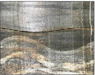
in Appendix B). An example section is presented in Figures 2.2 where the

verti-cal axis is depth and horizontally is the borehole circumference always oriented

starting from Magnetic North (left side of the image). Fracture and layer are

appearing in Figure 2.2.

2.1.2 Acoustic Imaging

High-resolution Acoustic Televiewer (HiRAT) provides high-resolution, oriented

(27)

[image:27.612.157.485.68.328.2]

Figure 2.2: Optical televiewer borehole logs sample

acoustic transducer and a rotating acoustic mirror to scan the borehole walls with

a focused ultrasound beam. The amplitude and travel time of the reflected

acous-tic signal are recorded simultaneously as separate image logs. Features such as

fractures reduce the reflected amplitude and often appear as dark sinusoid traces

on the log. The travel-time log is equivalent to a high-precision 360-arm calliper

and shows diameter changes within open fractures and break-outs. Directional

information is also recorded and used to orient the images in real time [4]. An

example section of acoustic borehole log is shown in Figure 2.3.

High resolution acoustic pulses -1.5 MHz frequency- are generated by a fixed piezo-electric resonator and then transmitted along the tool axis to be reflected

by a rotating planar mirror as shown in Figure 2.4. The beam is ultra-focused

to achieve highest resolution. After mirror reflection, the pulses propagate

or-thogonally to the probe body through the acoustic window (nylon construction

(28)

[image:28.612.148.493.66.329.2]

Figure 2.3: Acoustic borehole log [4]

wall of the borehole following an almost normal incidence. The reflected energy

is automatically picked up by the same transducer, in a reverse path, from which

the amplitude of the returned first reflections and the related elapsed two-way

travel time are recorded.

Typical logging speed is in the 1.5−5 m/minute range (to be constant). High vertical and horizontal resolution (i.e. 360 samples per rev) requires slow logging

speed. Logging too fast will result in incomplete borehole wall imaging (lack of

vertical resolution) with the resulting plots appearing compressed in the

acquisi-tion software. On the other side, logging excessively slowly does not result in a

better image, it only increases redundancy in the data stream and hence the

stor-age requirement. This is because any horizontal point might be imstor-aged by more

than one sweep of the acoustic beam (according to head speed and baud rate [4]).

(29)

[image:29.612.237.407.67.337.2]

Figure 2.4: Illustration of acoustic acquisition tool [4]

and opaque mud. The acoustic televiewer is more reliable for a wider variety of

applications, because it is often easier to use mud to keep fluid in the hole than to

either flush the hole clean, or empty it, or wait until the fluid clears up. Further,

the HiRAT can more easily detect the fine fractures [4].

2.1.3 Resistivity Imaging

The resistivity borehole imager, also called (Formation Micro Imaging FMI), was

developed for the oil market and is still mainly used there [31]. The resistivity

imaging have developed gradually from dip-meter tools and typically consist of

four to six arms with one or two conductivity pads attached that contain a

num-ber of resistivity buttons at the end of each arm. The pads are pressed against

borehole wall to measure the formation micro-conductivity [31] producing an

elec-trical image of the borehole.

(30)

sim-plicity, low cost of equipments and ease of use. FMI provides detailed information

of layers formations, identification of structural geology, fractures and rock

tex-tures [32].

The resistive FMI tool takes continuous circumferential micro-conductivity

measurements in the borehole, producing an electrical image of the borehole,

ori-ented with respect to North by means of a gyroscopic compass [31, 32]. Data are

processed and displayed as either a static (data equalised over the entire depth

range of the logging run) or dynamic equalisation (data equalised over a much

shorter window, usually 510 m), unrolled inside wall image, clockwise from 0◦

(North) to 360◦.

In this research a resistivity imaging tool form Roberson Geologging Ltd is

used. The tool includes 4 pads each containing twelve button electrodes mounted

on 2 pairs of powered arms [33]. Resistivity borehole data sample is shown in

Figure 2.5. In general yellow colours in resistivity log represents more resistive

rock type.

2.2 Data Pre-Processing

Pre-processing is an essential step in order to prepare collected borehole data for

subsequent processing. It is found that data pre-processing has a key role when

trying to build an automated interpretation system using computer algorithm.

The environment of drilled borehole (e.g. when borehole is flushed by a clear

fluid or it is full of mud) and the configuration of data acquisition system may

introduce a host of errors that can’t be accounted by manual interpretation. This

leading to degradation of the quality of the acquired borehole data, influencing the

(31)

[image:31.612.206.437.198.590.2]

(32)

with non-masked fracture. A series of pre-processing techniques including median

filtering, sub-sampling, decentralisation compensation and histogram equalisation

are performed in order to enhance the image quality. Due to the length of the

borehole image that varies from a few meters to hundreds of meters, the image

is partitioned into smaller parts in order to ease the processing.

2.2.1 Background Removal

Borehole image noise and clutter can be caused by the probe decentralisation

problem, the well is not cleaned very well after drilling process or the tool has a

stick/slip behaviour which is often due to varying well diameter. The clutter

ap-pears as vertical stripes or affect contrast quality of borehole data, and thus it will

affect the feature extraction and characterisation. Figure 2.6(a) shows an

exam-ple a poorly centralised acoustic sensor that appear as two parallel vertical strips.

It is possible to remove background or clutter by subtracting from the

bore-hole data an ensemble average of the borebore-hole data image over the region of

interest. Here it is assumed that the target indication are present in a relatively

small number of measurements and the mean of borehole data can be considered

to be a measure of system clutter. The image is divided into horizontal lines and

then the ensemble mean of each column of pixels intensities across each strip is

subtracted. Assume the unprocessed image y and win the size of strip starting from point jbg, the processed image ˆy(i) is calculated using

ˆ

y(i) = y(i)− 1

win

jbg+win−1

X

j=jbg

y(j) (2.1)

Image clutter may be removed by specifying the corresponding values of jbg

(33)

(a) Acoustic amplitude image, before background removal

(b) Acoustic amplitude image, after background removal

(34)

technique is particularly suited for instances where the fractures are

well-separated from system clutter, and affects on thin fractures detection accuracy.

2.2.2 Probe Decentralisation Correction

Detailed information about the borehole shape can be derived from the acoustic

travel-time image. As discussed in Section 2.1.2, the acoustic tool does not really

measure borehole calliper (continuous measurement of the size and shape of a

borehole along its depth) rather it measures multiple distances from the tool to

the borehole wall. Calliper is only defined with respect to the centre of a regular

shaped borehole.

Probe centralisation is fundamental to have high quality images, Robertson

Geologging Ltd brass centralisers work on the bowstring principle, with three or

four arms (depending upon the diameter and centralisation force required).

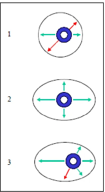
However, probe decentralisation affect on collected data. In Figure 2.7 three

different situation are schematically presented. In case 1, the tool is decentralised

in a circular borehole. The two green arrows indicate the two directions where

the acoustic beam hits the borehole wall perpendicularly. Only at these two

di-rections give maximum reflection amplitudes and the addition of the two opposite

travel-times gives the true borehole calliper. In the direction of the two red

ar-rows we measure a secant. The length of the secant depends on tool position. in

case 2, the beam is perpendicular to the borehole wall in four directions. Calliper

values can be calculated in all directions, because the tool is in the centre of the

borehole cross-section. In case 3, the tool is decentralised in an elliptical

bore-hole. The borehole wall is hit perpendicularly in four directions. But it is quite

obvious that the addition of the distance given by the red arrows and distance in

(35)

[image:35.612.236.407.94.405.2]

Figure 2.7: Probe decentralisation cases

To overcome probe decentralisation problem, the borehole shape should be

detected by mapping the travel-time data into distance data (y,x) relative to

the centre of the borehole in terms of radius (r) and angle (φ). This gives the possibility to accurately detect the movement of the tool from its actual position

to the centre of the borehole. Then proposed ellipse fitting process is performed

by using non-linear least squares function to find the borehole dimension. This

will be discussed in detail in Section 5.1.

2.3 Summary

This chapter has described different method for borehole data acquisition, these

(36)

acquisi-tion parameters, environment and data sample were presented.

Moreover, the pre-processing methods were presented to prepare the borehole

data in a format suitable for subsequent processing. The pre-processing include

background removal which enhances borehole data contrast, and solving of probe

decentralisation problem which affects borehole data readability. This prepares

(37)

Chapter 3 Visual Texture and Image

Segmentation

3.1 Introduction

In previous chapter borehole data is pre-processed and prepared for further

pro-cessing and feature detection. Due to the noisy nature of borehole data, the main

challenge is to find the texture boundaries even if the textured surface cannot

be classified, this problem can be solved using texture segmentation to obtain

a map of boundaries of similarity-textured regions. Defining texture boundaries

helps in extracting smooth edges in the next step of the proposed method (edge

detection) as shown in Figure 1.4.

Texture analysis methods have been utilised in a variety of application

do-mains. In some of the similar domains (such as remote sensing) texture already

has played a major role. In order to segment an image, it is important to extract

meaningful features that represent each segment accurately to enable

segrega-tion of the distinctive regions contained in the image. Visual texture is one of

(38)

surfaces with similar shape or colour. Texture, although recognised when seen,

is very difficult to define. This difficulty means that a single, unambiguous and

widely accepted definition does not exist. A reason for this is the strong intuitive

concepts of texture, which are hard to encompass fully in a formal definition.

3.2 Texture Properties

Texture can be recognised when seen but it is very difficult to define. This

dif-ficulty is demonstrated by the number of different texture definitions attempted

by vision researchers [34, 35]. Coggins [36] has compiled a catalogue of texture

definitions in the computer vision literature as listed below [37]:

“A region in an image has a constant texture if a set of local statistics or

other local properties of the picture function are constant, or approximately

pe-riodic.” [38]

“The image texture we consider is non-figurative and cellular... An image

tex-ture is described by the number and types of its (tonal) primitives and the spatial

organisation or layout of its (tonal) primitives... A fundamental characteristic of

texture: it cannot be analysed without a frame of reference of tonal primitive

being stated or implied. For any smooth gray-tone surface, there exists a scale

such that when the surface is examined, it has no texture. Then as resolution

increases, it takes on a fine texture and then a coarse texture.” [39, 40]

This collection of definitions demonstrates that the definition of texture is

for-mulated by different people depending upon the particular application and that

there is no generally agreed upon definition. Image texture, defined as a function

(39)

Figure 3.1: Processing stages of texture segmentation system

applications. Defining homogeneous regions in an image is the most important

application in visual texture and is called texture classification. The goal of

tex-ture classification is to produce a classification map of the input image where each

uniform textured region is identified with the texture class it belongs to [34, 41].

The second type of problems that texture analysis research attempts to solve is to

find the texture boundaries even if we could not classify these textured surfaces

and its calledtexture segmentation, the goal of texture segmentation is to obtain

the boundary map of homogeneous regions.

The stages of the segmentation technique adopted here are outlined in

Fig-ure 3.1. A segmentation is produced by integrating different textFig-ure featFig-ures. If

the texture features (to be described below) are capable of discriminating these

categories then the patterns belonging to each category will form a cluster in the

feature space which is compact and isolated from clusters corresponding to other

texture categories. The recovery, discrimination and labelling of such clusters is

performed by neural networks [5].

3.3 Texture Analysis Techniques

As there are a wide range of definitions, applications and concepts relating to

(40)

inter-preting texture. These methods can be broadly categorised into four classes:

1. Structural methods: they consider textures to have two fundamental components: a basic primitive (called a texel) that comprises the texture

and the spatial organisation of these primitives. Since this only allows the

description of very regular textures, the rules are often extended to become

statistical, which offers more freedom in the description [42]. The advantage

of the structural approach is that it provides a good symbolic description of

the image; however, this feature is more useful for synthesis than analysis

tasks.

2. Statistical methods: they do not attempt to understand explicitly the hierarchical structure of the texture. Instead, they represent the texture

indirectly by the non-deterministic properties that govern the distributions

and relationships between the grey levels of an image. These can be

first-order statistics (e.g. mean and histogram) and higher first-order statistics mostly

second-order. Gray-level-co-occurrence matrix is the most popular

statisti-cal method which proposed by Haralick [43].

3. Model-based methods: they attempt to characterise textures by con-structing a stochastic model, this can be done by fitting some analytical

function to the texture. In practice, the computational complexity arising

in the estimation of stochastic model parameters is the primary problem.

Gibs-Markov, Random filed and auto-regressive models are typical

exam-ples of these methods [44, 45].

4. Transform methods: represent the image into something more meaning-ful or in a new form in which textures can be detected more easily.

Mul-tiresolution methods are typical of these that transform images into a new

representation which separates features of different scale and resolution, and

(41)

According to the need of finding homogeneous regions in borehole data, and

extract non-distinct fracture and layers, which are located between different

re-gions at acceptable computational complexity. This research concentrate on

sta-tistical and multi-resolution methods, and investigate their applications in

bore-hole data characterisation.

3.4 Statistical Texture

Statistical texture analysis computes local features at each point in a textured

image, and derives a set of statistics from the distributions of the local features.

The local feature is defined by the combinations of intensities at specified

posi-tions relative to each point in the image. According to the number of points which

define the local feature, statistics are classified into first-order, second-order, and

higher order statistics [46]. The pioneering work of Julesz [47] concentrated on

these spatial statistic properties of the image gray levels [48].

The basic difference between first-order statistics and higher-order statistics

is that first-order statistics estimate properties (e.g.average and variance) of

in-dividual pixel values, ignoring the spatial interaction between image pixels, while

second and higher-order statistics estimate properties of two or more pixel values

occurring at specific locations relative to each other.

3.4.1 First-order Statistics

First-order statistics measure the likelihood of observing a gray value at a

ran-domly chosen location in the image. First-order statistics can be computed from

the histogram of pixel intensities in the image, these depend only on

individ-ual pixel values and not on the interaction or co-occurrence of neighbouring pixel

(42)

Assume a two-dimensional image function discretised into gray levels. The

occurrence probability of intensity iin the image is given by:

h(i) = θ(i)

A (3.1)

where θ(i) (i = 1,2, . . . , g) is the number of points whose intensity is i in the image and A is the area of the image (the total number of pixels in the image).

This distribution takes the form of a histogram. The histogram function is

computed for small, overlapping region and resulting distribution associated with

the centre pixel of the region because different image partition may have different

textures.

The following are the simple seven first-order texture measures that are

of-ten used to characterise the histogram: mean, variance, skewness, kurtosis,

fifth moment, histogram entropyand relative smoothness, are calculated as follows:

1. Mean:

µh = g

X

i=1

ih(i) (3.2)

2. Variance (second moment)

σ2_h =

g

X

i=1

(i−µh)2h(i) (3.3)

(43)

g

X

i=1

(i−µh)3h(i) (3.4)

4. Kurtosis (fourth moment):

g

X

i=1

(i−µh)4h(i) (3.5)

5. Fifth moment:

g

X

i=1

(i−µh)5h(i) (3.6)

6. Histogram entropy:

−

g

X

i=1

h(i) logh(i) (3.7)

7. Relative smoothness:

1− 1

1 +σ2

h

(3.8)

The distribution mean µh is not considered as an independent feature, as

there is no observed correlation between it and the different texture categories,

it is computed in order to compute the further features.

Each measure is a function of the pixel intensity distribution h(i) within any (N ×N) region centred at any arbitrary point (x, y). These square windows are shifted across the image in a small increment of size, where (≥1). This finite increment makes it necessary to associate the texture feature value with an×

square centred around (x, y). The result of features matrices represent points that have some relationship to the probability distribution function of pixel intensities

(44)

(a) Image of a fingerprint

(b) After addition of border

Figure 3.2: Example of the reflected image border to overcome the difficulty in computing boundary features

boundaries so these point will not be mapped. To overcome this problem, the

image is surrounded with a reflected replica of the image border, of thickness

N/2, as shown in Figure 3.2. A value of N = 20 was chosen in order to capture the variations in fracture amplitude, and a value of 5 was assigned to, resulting in 75% adjacent window overlap.

Although first-order statistics provide features descriptions, it might not be

enough for the discrimination process. As demonstrated by Julesz [47], two

tex-tures could have identical first-order statistics, because these measures may not

carry any information regarding the relative positions of pixels with respect to

each other. This limitation can be overcome by using of of second-order

statis-tics [48–50].

3.4.2 Second-order Statistics

Second-order co-occurrence texture features are defined as the likelihood of

ob-serving a pair of gray values occurring at the endpoints of a dipole (or needle) of

(45)

are properties of pairs of pixel values. It was first introduced by Haralick [39, 43]

in the seventies, and it was found that the co-occurrence features is the best with

regards to texture classification performance for the experimental results that

were presented in [51, 52].

Co-occurrence textural features are computed based on gray-tone spatial

de-pendencies. Assuming a position operator ∆ = (∆x,∆y), joint probability

ma-trixP∆ and joint probability of the existence of a pair of pixels with intensities i

and j existing at separation ∆ is denoted by P∆(i, j). P∆ is calledgray level

co-occurrence matrix or simply(GLCM), This matrix depends both on the angular relationship between pixels and the distance between them. Matrix manipulation

allows the co-occurrence matrix to be computed in a fast and efficient manner.

For any particular position operator ∆ one can define a large number of

de-scriptors or features that characterise the or features that characterise the content

of P∆. From the abundance of features available, previous studies(e.g. [51, 53])

recommend to use the following eight features [54]:

1. The maximum probability gives an indication of the strongest response

to ∆:

maxi,jP∆(i, j) (3.9)

2. The element-difference third-order moment:

g

X

i=1

g

X

j=1

(46)

3. The inverse element-difference second-order moment: g X i=1 g X j=1

P∆(i, j)

(i−j)2 (i6=j) (3.11)

4. Energy or the angular second moment, which is a measure of uniformity,

and is alternatively referred to as inertia:

X

P∆(i, j)2 (3.12)

5. The correlation is a measure of linearity:

Pg

i=1

Pg

j=1ijP∆(i, j)2−µxµy σxσy

(3.13)

where:

µx = g X i=1 i g X j=1

P∆(i, j) (3.14)

µy = g X j=1 j g X i=1

P∆(i, j) (3.15)

σx = g

X

i=1

(i−µx)2 g

X

j=1

P∆(i, j) (3.16)

σy = g

X

j=1

(j −µy)2 g

X

i=1

P∆(i, j) (3.17)

6. Entropy is a measure of randomness:

− g X i=1 g X j=1

(47)

7. Homogeneity is defined as: g X i=1 g X j=1

P∆(i, j)

1 +|i−j|2 (i6=j) (3.19)

8. Contrast is a measure of the amount of local variations present in the image

window: g X i=1 g X j=1

(i−j)2P∆(i, j) (3.20)

The above eight features when multiplied by the number of possible values

of ∆ for which the co-occurrence matrix can be computed leads to a potentially

large number of dependent features. As there have been no clearly-established

guidelines for the selection of ∆, the correct choice for this operator is usually

achieved on a trial-and-error basis. A value of (3,3) has been used in this study and has achieved satisfactory results with the borehole images in question. In

addition to the eight features calculated above, a two-dimensional entropy

mea-sure has been utilised, because it has proven to be effective as texture feature as

proposed in [55, 56].

The proposed histogram is a (gray-level/local average gray-level)g×g scatter-plot, each bin of which is related to the frequency of occurrence of the particular

(gray-level/average) pair within the 5×5 pixel window. The a priori-probability

h2(i, j) of an intensity pair (i, j) is given by the total number of occurrences of

the pair divided by the total number of pixels. The total entropy for this 2−d

(48)

−

g

X

i=1

g

X

j=1

h2(i, j) logh2(i, j) (3.21)

The result are in a total of 15 statistical texture features images, these images

are normalised to have zero mean and unity standard deviation. This avoids

system bias to the large numerical range, then the images are stacked together in

3-dimensional matrix as in Figure 3.3. Each pixel in the original image is mapped

into 15-element feature vector.

Figure 3.3: Formation of feature vector from feature images

The list below summarise the 15 statistical texture features image:

1. Histogram variance

2. Histogram skewness

3. Histogram kurtosis

(49)

5. Histogram relative smoothness

6. Histogram entropy

7. Co-occurrence correlation

8. Co-occurrence maximum probability

9. Co-occurrence third-order difference moment

10. Co-occurrence second-order inverse difference moment

11. Co-occurrence entropy

12. Co-occurrence uniformity

13. Co-occurrence contrast

14. Co-occurrence homogeneity

15. Two-dimensional entropy

3.5 Mutiresolution Texture

The approach adopted here is multi-channel filtering, and it is a more recent

approach to texture analysis, inspired by multi-channel filtering theory for

pro-cessing of visual information in the early stages of human visual system [57, 58].

Various cells within the visual cortex can perform different types of processing

on the incoming signal. It has also been proven that the human visual system

decomposes the retinal image into a number of filtered images, each image

con-tains intensity variations over a narrow range of frequency and orientation [5].

A multi-channel filtering technique projects the image onto a set of

(50)

Figure 3.4: Stages of multi-resolution texture segmentation procedure

Wavelet transform. This generates a descriptor for each image pixel. Neural

net-works techniques are then used to segment the image as shown in Figure 3.4.

3.5.1 Gabor Filter

In their simplest form, Gabor functions are harmonic oscillations modulated by a

Gaussian probability pulse. These elementary signals are localised in time and in

frequency and possess the important property of minimising the combined

effec-tive spread in both time and frequency. Gabor signals have been proven [59] to

provide dual space/spatial-frequency dependence simultaneously and model very

well the spatially localised receptive field of visual cells [60].

A two-dimensional symmetric Gabor filter can be defined as a sinusoidal plane

wave of some frequency and orientation modulated by a 2-D Gaussian envelope.

The impulse response of a complex canonical Gabor filter in the spatial domain

is given by:

g(˘x,y˘) = _p1 2πσg

exp −1 2 ˘ x2 σ2 x

+ y˘

2

σ2

y

.cos (−2πu0x˘+ρ) (3.22)

(51)

and σy are the space constants of the Gaussian envelope along the x and y-axes

respectively [61–63], and σg is equal toσx,σy and ˘xand ˘y are the oriented xand y co-ordinates after undergoing a rotation by an arbitrary angle α using Equa-tion 3.24.

Selection of σx and σy determines the resolution in both spatial and

spatial-frequency domains. Low values of σx and σy favour spatial resolution, and high values favour spatial-frequency resolution. When segmenting an image, short

spatial intervals are preferable because one wishes to approximate the boundary

between textures. However smaller frequency bandwidths are preferable to make

better distinctions between different textures. The main challenge is the inverse

relation between spatial-frequency and the spatial extent, this known by the

un-certainty principle.

The Fourier spectrum of a Gabor function of radial frequencyu0 and

orienta-tion α is a pair of real-valued Gaussian, centred in the spatial-frequency domain at radial distances (proportional to)u0 and −u0 from the origin, and oriented at

(an angle proportional to) the filter orientation α. When the phase is zero, the Fourier transform of the real component of the even-symmetric Gabor function

g(x, y) above is given by:

G(u, v) = 2πσxσy

exp−1 2

(u−u0)2

σ2 u + v 2 σ2 v

+ exp−1 2

(u+u0)2

σ2 u + v 2 σ2 v (3.23)

whereσu = ₂_πσ1_x and σv = ₂_πσ1_y, and ˘u and ˘v correspond to the spatial frequency

(52)

Table 3.1: Filter parameters for Gabor filter bank

Filter number

Parameter 1 2 3 4 5 6 7 8 9 10 11 12

σx/x size 1 1 1 1 1 1 1 1 1 1 1 1

σy/y size 1 1 1 1 1 1 1 1 1 1 1 1

u0 1 1 1 1.5 1.5 2 2 2.5 2.5 3.5 3.5 3.5

α(◦) 10 90 170 60 140 50 130 20 100 10 90 170

ρ(◦) 0 0 0 0 0 0 0 0 0 0 0 0

   ˘ x ˘ y   =   

cosα sinα

−sinα cosα

  ·    x y    (3.24) Hence, ˘

x=xcosα+ysinα (3.25)

and

˘

y =−xsinα+ycosα (3.26)

The illustration of the effects of varying the orientation of the filter on the

corresponding spectra, radial frequency and Gaussian space constants are shown

in Figure 3.5.

Various of filters are constructed and the configurations are summarised in

Table 3.1, with the aim of a uniform coverage of the spatial-frequency plane.

Filters were selected with orientations varying from 10◦ to 170◦ in steps of 20◦,

and with radial frequencies one octave apart from 1 to 8 cycles/image-width.

Although this filter set comprising 9×4 = 36 filters gave satisfactory results,

experimental variations were made on this initial set in order to reduce the number

of filters and thus reduce the data and the processing time. It was observed

that the low-frequency filters were more effective in distinguishing the required

textures, and a modified filter set was composed, comprising of only 12 filters,

(53)

(a )

( b )

( c )

( d )

( e )

g ( x )

g ( x )

x

u

G ( u ) G ( u )

g ( x )

x _u

G ( u )

1

- 1

1

- 1

- ½ ½

s = 1 / ( 2 p )

s _u = 1 / ( 2 p )

u 0 = 1

s = 1

u 0 = 1

s _x = ½ s u = 1 /p

u 0 = ½

s _x = 1

u 0 = 1

s _x = 1

s _y = 1 a = 0

u 0 = 1

s _x = 1

s _y = 1

a = 4 5 o

4 5 o

g ( x , y )

G ( u , v )

(54)

3.5.2 Filtering

The filtering operation is performed in the spatial domain, by convolving each

filter functiongi(x, y) with the image f(x, y) as follows:

hi(x, y) = |gi(x, y)∗f(x, y)| (i= 1,2, . . . ,12) (3.27)

Each pixels magnitude reveals the relative strength of the variations

charac-terised by the filter attributes in its neighbourhood in the original image. Since

these filters have the property of achieving the optimum localisation in both

domains, each filtered image shows the best possible distribution of the spatial

signals within the given bandwidths of the corresponding filter.

The filtering operation results in a set of 12 independent 256×256 filtered

images, stored in a 3-dimensional matrix. In order to keep the intensities of

the outputs from all the filters within a common range, each image was then

normalised to have zero mean and unity standard deviation.

3.5.3 Feature Computation

Before segmentation can be performed, a set of texture measures or features must

be developed from these filtered images. As suggested in [64], attributes of blobs

in these images can be captured by applying a non-linear transformation in order

to transform the sinusoidal modulations to square modulations. The non-linearity

employed is the hyperbolic tangent as suggested in [65]. This blob image can then

be analysed and local measures computed and used as features. The local energy

is used as a texture feature as suggested in [5], generating one feature image per

(55)

intensity variations in the image, which is in turn related to the Gabor filter

centre frequencyu0 as in [66]:

σω = κω u0

(3.28)

where the constant κω is chosen (empirically) as 0.5 image-widths/cycle.

Al-though the choice of parameters above was adopted, it has been noted that

vari-ations in the values of bothα andκω of up to 50% produced a little effect on the

overall performance of the segmentation.

The resulting 12 images are the multi-channel feature set, they are used for

the formation of a 12× (M ×N) feature matrix, where [M, N] are equal to the input image dimensions, with each column representing a feature vector.

The statistical and multi-channel features are then combined to form a set of

12 + 15 = 27 texture stacked images.

3.6 Number of Clusters

Depending on how descriptive the input features are of the underlying data, they

contain inherent clusters corresponding to the different categories, ideally each

cluster is compact and isolated from clusters corresponding to other categories.

Clustering algorithms identify densely populated regions in feature space and

as-sign class membership labels to each data point. The success of a classifier is

directly related to the degree of clustering and the separation between clusters.

In order to segment the image into regions representing different clusters with

different visual texture, it is important to be able to determine automatically

(without a priori knowledge) the number of clusters depicting each image

(56)

the most venerable problems in cluster analysis, and several indices have been

proposed to provide such an estimate [67, 68]. An internal index of partition

adequacy compares the given proximity matrix with the partition of the objects

obtained from a cluster analysis without reference to category labels or other

external information.

The modified Hubert (MH) index proposed by Dubes [67, 69] has proven to

perform significantly better than other such indices, and with higher reliability.

This index was thus adopted to determine the number of clusters in the borehole

data. Adapted from the Hubert gamma statistic [70, 71], this index is the point

serial correlation coefficient between the matrix of inter-pattern distances and the

distances recovered from the clustering solution.

A clustering solution is a partition {C1, C2, . . . , Ck} of the integers from 1 to msuch that i∈Ck if ini is in the kthcluster. The centre of Ckis denoted by the

d−place vector:

mk =

1

mk

X

i∈Ck

ini (3.29)

where mk is the cardinality of Ck and

m=

d

X

k=1

mk (3.30)

The Euclidean distance d−place vectors in and y is defined as:

kin−yk=p(in−y)T₍_in₋_y₎ _(3.31)

(57)

L(i) =k if i∈Ck (3.32)

with M =m(m−1)/2,

r = 1

M m−1

X

i=1

m

X

j=i+1

kini−injk ·m_L₍_i₎−m_L₍_j₎

(3.33)

Mp =

1

M m−1

X

i=1

m

X

j=i+1

kini−injk (3.34)

Mc =

1

M m−1

X

i=1

m

X

j=i+1

m_L₍_i₎−m_L₍_j₎

(3.35)

σ_p2 = 1

M m−1

X

i=1

m

X

j=i+1

kini−injk2−M_p2 (3.36)

σ2_c = 1

M m−1

X

i=1

m

X

j=i+1

mL(i)−mL(j)

2

−M_c2 (3.37)

The MH measure for clustering{C1, C2, . . . , Ck} is:

M H(k) = r−MPMc

σpσc

(3.38)

As observed by Dubes [67], when the data contains a strong clustering, the

MH index statistic increases monotonically as the number of clusters increases,

and then levels off with “significant knee” formed at the true number of clusters.

The index will be 1 for the trivial clustering in which each pattern is an

individ-ual cluster, and is not defined for a one-cluster clustering. A decision rule is thus

(58)

from 2 tokmax, where kmax is the maximum estimated number of clusters in the

data.

Suppose the true number of cluster is ktrue. The clusterings with k > ktrue

will be formed by breaking the true clusters into smaller ones, and as a result

the correlation between kini−injk and

m_L₍_i₎−m_L₍_j₎

matrices will be high.

The clusterings with k < ktrue clusters, however will be formed by merging the true clusters, hence reducing the correlation. Therefore, assuming that the

tex-ture featex-tures provide strong discrimination between different textex-ture categories,

a significant knee should be observed in the plot of MH(k) at the true value ofk.

The knee function atkclusters,S(k) is the tangent of the acute angle between the lines defined byM H(k+ 2),M H(k+ 1) andM H(k). The larger this tangent, the more significant the knee at k clusters. Although the first significant knee

can be detected by setting a threshold of significance, it may also be sought by

eye. Figure 3.6 demonstrates this knee at four categories for the borehole visual

texture features.

3.7 Representative Categories for Image Data

As discussed in Section 3.6, and Figure 3.6 shows image data (Figure 3.7)

con-tains four different textures or visual properties. Hence in all subsequent analysis

and investigation, the data is considered to consist of four categories of texture.

Typical patches that represent four categories are selected to perform

quanti-tative analysis of borehole data. Patches of (32×32) pixels were selected

manu-ally from borehole image (e.g Figure 3.7), and compiled together in the form of

(59)

Figure 3.6: Plot of MH index versus number of categories showing significant knee at four classes in Figure 2.2

composite image which correspond to the four selected image categories will be

used for classifier training and for performance estimation.

3.8 Competitive Learning

In competitive learning, an input vectors is classified into one of K categories based on detected cluster in training set in. The network weights are organised during rejected dissimilar vectors, and the most similar or called winner is

ac-tivated for weight building. When the network is trained correctly, all cluster

members ini will have the same winner. Kohonen network is called on the net-work to be trained and as shown in Figure 3.9.

The process of dividing the input space into a number of adjacent subspaces

(60)

Figure 3.7: Patches selected from borehole image, representative of different visual textures

Automatic feature detection and interpretation in borehole data