Effects of turbulence modelling on prediction of flow characteristics in a bench-scale anaerobic gas-lift digester

(1)

Effects of turbulence modelling on prediction of ﬂow characteristics

in a bench-scale anaerobic gas-lift digester

A.R. Coughtrie

⇑

, D.J. Borman, P.A. Sleigh

School of Civil Engineering, University of Leeds, Leeds LS2 9JT, UK

h i g h l i g h t s

Flow in a gas-lift digester is investigated using computational ﬂuid dynamics. The effect of four RANS turbulence models on the ﬂow characteristics is shown. The Transition SST turbulence model is determined to be most accurate for this case. ANSYS Fluent and OpenFOAM are used to show solver independence.

The accuracy of a singlephase approximation is examined using a multiphase model.

a r t i c l e

i n f o

Article history:

Received 21 December 2012

Received in revised form 21 March 2013 Accepted 24 March 2013

Available online 6 April 2013

Keywords:

Anaerobic digestion CFD

Turbulence modeling Gas-lift

Multiphase

a b s t r a c t

Flow in a gas-lift digester with a central draft-tube was investigated using computational ﬂuid dynamics (CFD) and different turbulence closure models. The k-xShear-Stress-Transport (SST), Renormalization-Group (RNG) k-

, Linear Reynolds-Stress-Model (RSM) and Transition-SST models were tested for a gas-lift loop reactor under Newtonian flow conditions validated against published experimental work. The results identify that flow predictions within the reactor (where flow is transitional) are particularly sensitive to the turbulence model implemented; the Transition-SST model was found to be the most robust for capturing mixing behaviour and predicting separation reliably. Therefore, Transition-SST is recommended over k-

models for use in comparable mixing problems. A comparison of results obtained using multiphase Euler–Lagrange and singlephase approaches are presented. The results support the validity of the singlephase modelling assumptions in obtaining reliable predictions of the reactor flow. Solver independence of results was verified by comparing two independent finite-volume solvers (Flu-ent-13.0sp2 and OpenFOAM-2.0.1).

1. Introduction

The desire to extract the embodied energy from within what are currently waste products has driven the increased use of anaerobic biogas digesters. As a result the stability and efﬁciency of the digesters has become of greater concern. The process of anaerobic digestion turns organic wastes into methane, carbon dioxide (biog-ases) and an organic waste product of reduced volume, with a low-er pathogen load than the original matlow-erial. The biogas produced from a fully operational stable digester is expected to be approxi-mately 65% methane and 35% carbon dioxide by volume, this gas can then be used as fuel to heat the digester and other parts of the biogas plant or in the generation of electricity (Taricska et al., 2009). A number of different factors affect the stability of anaerobic digesters (AD’s) including the temperature, substrate content and

mixing of the slurry during digestion. For example, how well mixed the slurry is will affect the pH distribution throughout the digester; methane producing bacteria are highly sensitive to pH and even small variations can have a substantial effect. Mixing is also useful in preventing settling of suspended biomass and the build-up of a scum layer on the slurry surface which can inhibit the escape of the biogas. As such, a well-mixed homogenous slurry is necessary for stable, controlled anaerobic digestion (Turovskiy and Mathai, 2006).

Due to the nature of the slurries used in the digesters and the size of full scale industrial plants, experimental methods of deter-mining the flow characteristics are expensive and complicated. Computational fluid dynamics (CFD) provides an excellent method of assessing the flow characteristics and mixing effectiveness un-der different digester configurations without the time and expense of experimental studies. Over the past 20 years, research work describing numerical modelling of anaerobic digesters has been undertaken widely; with CFD being used to assess the mixing in

http://dx.doi.org/10.1016/j.biortech.2013.03.162

⁄ Corresponding author. Tel.: +44 1133433292.

E-mail address:[email protected](A.R. Coughtrie).

Contents lists available atSciVerse ScienceDirect

Bioresource Technology

(2)

anaerobic digesters of different types. This includes assessment and development of CFD procedures for use with mechanically mixed digesters (Wu, 2010a; Joshi et al., 2011; Bridgeman, 2012). Modelling of mechanically mixed digesters has shown that the type of impeller and flow direction effects the mixing efficiency, with up mixing being found to be more efficient than down (Wu, 2010b; Aubin et al., 2004). Yu et al. (2011) also investigated mechanically mixed AD’s and showed the potential of helical rib-bon impellers in the mixing of high solids digesters and provided insight into the minimum power requirements. Additionally high solids AD’s typically contain slurries of a non-Newtonian nature which have been shown to produce significantly different flow pat-terns to Newtonian fluids when modelled (Wu and Chen, 2008). Numerical modelling has also been used to investigate flow and mixing in gas lift digesters, using tracers in full scale AD’s to mon-itor mixing time and showing that for internal loop gas lift AD’s transient oscillatory behaviour can sometimes be found ( Terashi-ma et al., 2009). Oey et al. (2003) showed that CFD modelling can be used to predict flow patterns in gas lift AD’s.Mudde and Van Den Akker (2001)described how such modelling can be used to design and tune gas lift AD’s andKarim et al. (2007)used CFD to alter the flow characteristics and reduce the stagnation region, by modifying the geometry of a bench scale anaerobic gas lift digester. There has however been no definitive methodology produced defining the most appropriate models and approach to use in pre-dicting the complex flow in anaerobic digesters. One of the signif-icant factors is that slurry being mixed in many bioreactors, including bench scale reactors from where experimental data is of-ten obtained, has Reynolds numbers indicating flow to be in the transitional turbulent region. This type of flow is known to be difficult to model and many common turbulence models fail to correctly resolve the flow field. This is compounded by the non-Newtonian nature of many slurries which can significantly alter Reynolds numbers throughout the digester where internal shear stresses vary. Published literature has not fully addressed the issue of which turbulence models are appropriate, nor what criteria should be adopted in selecting one for slurries of particular

rheology. Failure to simulate turbulence correctly in non-Newto-nian, transitional ﬂow regimes may result in an inability to capture the important ﬂow characteristics responsible for mixing reliably. There have been a small number of studies into the effects of tur-bulence modelling on the CFD results for anaerobic digesters (Wu, 2010b, 2011; Joshi et al., 2011; Bridgeman, 2012). The majority of CFD modelling of anaerobic digesters tend to rely on the standard k-

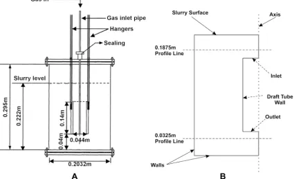
turbulence model with wall functions (Vesvikar and Al-Dah-han, 2005; Meroney, 2009; Mudde and Van Den Akker, 2001; Oey et al., 2003). Often little justification for this choice is given and may be due to it being a good general purpose turbulence model which has been found suitable for a wide range of flows. This is not however the case where transitional flows occur, a fac-tor which has been overlooked in previous studies. This approach impacts on the reliability of solutions as there is potential for sig-nificant variability in predictions for key phenomena, such as sep-aration points, and thus stagnation zone size. Reduced accuracy in solutions may result, with the k-

being shown to delay or fail in predicting wall separation resulting from adverse pressure gradi-ents (Menter, 2011). As such, the first part of this study was fo-cused on determining the factors affecting the choice of turbulence model in gas recirculation digesters; particularly in re-gard to low Reynolds number (Re) flow, transitional flows and boundary layer separation. Additionally, a comparison was made between results for two alternative, finite volume based, CFD solv-ers (ANSYS Fluent 13.0sp2 and OpenFOAM 2.0.1) in order to assess the solver independence of the predictions.

[image:2.595.81.507.478.738.2]

There are a number of options available when simplifying the multiphase gas driven digester problem for CFD to reduce the com-putational expense.Karim et al. (2007)used an empirical approx-imation for the flow at the top and bottom of the draft tube of their digester reducing the model to a singlephase problem by neglect-ing the flow in the draft tube. This assumes that the gas hold up (i.e. the dispersed gas volume fraction (Sieblist and Lübbert, 2010)) is not significant in the main annular section of the digester (seeFig. 2.1), allowing for the gas-phase to be neglected and an empirical fluid velocity formulation applied at the top of the draft

(3)

tube. The results of which were shown to have reasonable qualita-tive agreement with a comprehensive experimental study under-taken by the same authors (Karim et al., 2004). The same reactor geometry and modelling assumptions were used in this work, with the objective of providing comparison of turbulence models for a case where reliable experimental data exists for validation. Finally, a multiphase Euler–Lagrange model was implemented to more completely model the reactor physics. This more computationally intensive method allows the gas to be accounted for directly and attempts to eliminate inaccuracies that may be found in the single-phase approach.

All computational results were verified through comparison with the experimental results ofKarim et al. (2004). Axial velocity profiles at 0.1875 and 0.0325 m as well as visual qualitative com-parison between flow fields were used to assess accuracy of the model solutions.

2. Methods

2.1. Geometry

The digester geometry (Fig. 2.1) consists of a main annular sec-tion with a central draft tube suspended above the base of the tank. The gas passes down a central tube and is released as bubbles at the bottom of the draft tube, these bubble then rises to the slurry surface driving the ﬂow circulation.

2.2. Governing equations

The equations governing the flow of singlephase fluids are the well-known Navier–Stokes equations. For low speed flows (Mach < 0.3), where compressibility effects can be ignored, the density can be considered constant and the full continuity and momentum equations simplify for Newtonian fluids to the incom-pressible Navier–Stokes equations (Eqs.(2.1) and (2.2)).

r

v

¼0 ð2:1Þ

q

ð @

v

@t

|{z}

unsteadyacceleration

þ

v

_{|fflfflffl{zfflfflffl}}r

v

convectiveacceleration

[image:3.595.312.561.700.753.2]

Þ ¼ rp

|fflffl{zfflffl}

pressuregradient þ

l

r2

v

|fflfflffl{zfflfflffl} viscosity þ f |{z} otherbodyforces ð2:2Þ

where

q

is density,

v

the velocity vector,pthe pressure and

l

the dynamic viscosity. Additionally, in order to resolve the effect of tur-bulence ﬂuctuations at the very small scales without incurring pro-hibitive computational expense, time averaging of the equations can be performed, resulting in the Reynolds Averaged Navier– Stokes (RANS) equations (Blazek, 2005).

2.3. Turbulence modelling

The RANS equations contain additional Reynolds stress terms which mean the equations are not fully closed (there are more unknowns than equations) and require a turbulence closure mod-el to provide these extra equations (Menter, 2011). Through the use of the Boussinesq approximation relating the Reynolds stresses to the mean ﬂow the commonly used two equation eddy viscosity models are formed. The k-

and k-

x

are two such mod-els which provide a good compromise between performance and accuracy.

From the work performed byKarim et al. (2004)it can be seen that there is separation of the boundary layer at the outer wall of the digester and reattachment at the draft tube wall. Boundary layer separation is a common feature in many reactors and is prob-ably the most complex and important flow characteristic in this di-gester. The point of separation in the flow predicted at the outer wall, has a significant effect on the size of the recirculation zone.

The prediction of ﬂow separation and Laminar-Turbulent transition has for a long time been difﬁcult to capture using turbu-lence models which have a tendency to over or under predict these points in the majority of situations. The standard k-

model has been consistently found unsuitable for use in accurately modelling low-Re turbulent ﬂows or the separation of turbulent boundary layers effectively; this resulted in attempts to develop more accu-rate formulations such as the k-

x

SST model (Menter et al., 2003). These RANS turbulence models are particularly sensitive when close to walls and the effect of the approach taken when modelling near these boundaries can be significant. The no-slip condition used on solid walls creates a boundary layer that has a significant effect on the flow characteristics close by. There are several meth-ods that can be used to take this effect into account; the simplest and cheapest in terms of computational expense is the use of wall functions. Wall functions use empirical formulations to model the near wall flow where the k-

model is known to fail. They are how-ever only valid for mesh densities where theY+_{(a dimensionless} wall distance dependent on the distance to and friction velocity at the nearest wall and the local kinematic viscosity) falls within certain values. As such it is desirable to use a near wall treatment that is independent of theY+_{value. The SST k-}

_x

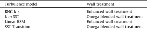
_{model uses a near} wall treatment that shifts between a viscous sublayer model (VSM) at smallY+_{values and wall functions at}_Y+_{values where the VSM is} invalid (Menter et al., 2003). A variation on this blended near wall treatment is also available for epsilon based two-equation turbu-lence models in the form of the enhanced wall treatment in Fluent 13.0sp2. ThisY+_{independent wall treatment is more attractive in} terms of mesh refinement studies, posing no restrictions on the refinement near walls and also allows the same turbulence model to be used when scaling up digesters where it is difficult to obtain lowY+_values.

In the work presented here four RANS turbulence models were applied to the problem being studied (Table 2.1). The k-

x

SST mod-el was chosen due to its ability to predict boundary layer separa-tion more accurately than the k-

models. A modiﬁcation to the standard k-

model was also applied; the RNG (Re-Normalisation Group) k-

has been found to predict streamline curvature with greater accuracy than other k-

models and may therefore be able to pick up on the complex ﬂow characteristics of the reactor. Addi-tionally a Reynolds Stress Model (RSM) model and the recently for-mulated Transition SST model (Menter et al., 2006) a ﬁve and four equation model respectively were used to see whether the addi-tional complexity of the models provides a comparable increase in the solution accuracy.

2.4. Euler–Lagrange multiphase modelling

Karim et al. (2007)made the assumption that the gas holdup in the annular section of the digester was negligible and so reduced their model to a singlephase approximation of the experimental di-gester. This simpliﬁcation although reducing the complexity and computational expense of the model does not take into account any of the more localised effects of the bubbles, particularly, di-rectly above and below the draft tube. Additionally, the approxi-mation used at the top of the draft tube for the ﬂuid velocity

Table 2.1

Turbulence models and respective wall treatments.

(4)

does not in any way account for the flow at the bottom of the draft tube. In order to account for any localised flow features formed by the bubbles a mathematical model that can simulate the multi-phase nature of the bubble driven flow is needed.

Euler–Lagrange multiphase modelling assumes one ﬂuid phase is solved using the Navier–Stokes equations with additional dis-persed phases (e.g. sand particles, bubbles, etc.) being modelled as particle packets. These dispersed particles are modelled by inte-grating the force balance on the particles in the Lagrangian refer-ence frame (Brebbia and Mammol, 2011). Eq. (2.3) is the force balance equation for the CartesianX coordinate, where the drag force (FD) is described by Eq.(2.4).

dub

dt ¼FDðuubÞ þ

gxð

q

b

q

Þ

q

b

þFvmþFp ð2:3Þ

FD¼

18

l

q

bd

2

b

CDRe

24 ð2:4Þ

where subscriptbrepresents the bubble and no subscript the ﬂuid phase,uis the velocity,gxgravity,

q

the density,

l

dynamic viscos-ity, d the diameter, CD the bubble drag coefficient and Re the Reynolds number. The last two terms in Eq.(2.3),FvmandFp, are additional force terms specific to bubble driven flow. Fvm is a virtual mass force which accelerates the fluid surrounding the particles according to Eq. (2.5) and is applicable where

q

b. Fp, represents the effect of pressure gradients and described by Eq.(2.6).

Fvm¼

1 2

q

b

d

dtðuubÞ ð2:5Þ

Fp¼ ð

q

b

Þubi @u

@xi ð

2:6Þ

2.5. Computational domain and boundary conditions

The computational domain used to approximate the fluid in the digester consists of an axisymmetric section taken as a slice through the digester. There are five separate distinct boundary conditions that can be applied to the numerical model. As dis-cussed (Section2.4),Karim et al. (2007)simplified the model by neglecting the gas phase and assuming a velocity inlet at the top of the draft tube with a uniform velocity profile. As the bubble col-umn in the draft tube is not being modelled, an approximation to its driving force effect is needed. The equation describing fluid velocity (U) developed byKojima et al. (1999)for short size draft tubes Eq.(2.7)is used.

U¼0:401

v

G

DT

DiD

!2

8 < :

9 = ;

0:564 ðD2

TD o2

DÞ

DiD2

( )0:182

L0:283

H0:0688

ð2:7Þ

Simpliﬁed byKarim et al., (2007) for this case to:

U¼0:401

v

G

DT

Di D

!2

8 < :

9 = ;

0:564

ðD2TD o2

DÞ

Di2

D

( )0:182

ð2:8Þ

where

v

Gis the superﬁcial gas velocity,DTis the tank diameter,DiD the tube inner diameter,Do

[image:4.595.44.544.68.358.2]

(5)

this case the central boundary condition was the axis. The walls of the digester are modelled with a no slip condition.

The most complex of the boundaries to specify is that repre-senting the free-surface of the slurry where it meets the collected methane gas. Under realistic physical conditions this interface can be considered to have some movement in all three axes. As we are assuming no angular flow no movement into the plane is allowed; further simplification can be made by assuming the surface as hav-ing a constant level. In such a case it is simple to model the bound-ary as having a zero shear and so allow the fluid to flow freely along the surface as would generally be the case at the slurry/gas interface. The impact of this is expected to have negligible effect on the overall flow field.

The spatial discretization scheme used for all the equations being solved (continuity, momentum and turbulence equations) was the third order MUSCL scheme and was run as a steady state simulation. Two widely used ﬁnite volume based CFD codes were used to determine the solver independence. The majority of the solutions presented were obtained using ANSYS Fluent 13.0sp2 while OpenFOAM 2.0.1 was used to check for and demonstrate independence. As far as is possible both solvers use the same set-tings for boundary conditions, turbulence model and discretization scheme.

3. Results and discussion

3.1. Mesh independence

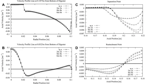
Fig. 3.1shows the mesh independence of the solutions where ‘m’ and ‘n’ are the horizontal and vertical cell counts. The meshes for all solutions shown were fully structured using square ele-ments. Four different mesh densities were based on scaled values of ‘m’ and ‘n’.Table 3.1 shows the mesh statistics including the average wallY+_{values for the mesh with the k-}

_x

_{SST turbulence} model.

When using the k-

x

based turbulence models aYþ_{1 is}

desir-able (though not essential), keeping the node of the ﬁrst element fully within the laminar layer so that the solution can be integrated to the wall. A standard method of determining whether a solution is mesh independent is the Grid Convergence Index (GCI), detailed methodology can be found inCelik et al. (2008). The GCI is used to report the discretization error and the apparent orderpof the solu-tion method. The calculasolu-tions were performed using the area aver-aged velocity magnitude of the solution domain. The apparent orderp of the solution method was calculated as 2.304. Three GCI values were determined for the four meshes, GCI21

fine¼0:19%;GCI 32

medium¼0:49%;and GCI 43

coarse¼0:83%. The small value of GCI shown for the 160200, 71200 and 17800 ele-ment meshes indicates that mesh independence is achieved with the 17800 element mesh.Fig. 3.1show axial velocity proﬁles at locations just above the inlet (A) and just below the outlet (B) (in a similar way toKarim et al. (2007)). These plots show agreement with the GCI indicating that the solution may be deemed mesh independent on the mesh of 17800 elements. However, the point where the solution separates from the outer wall and reattaches at the draft tube wall, as shown in the plots ofFig. 3.1(C) and (D)

shows that the solution is more sensitive at the wall and that inde-pendence can only be reasonably assumed with a mesh of 71200 elements. This increase in mesh density also has the advantageous effect of reducing the averageY+_{value to less than 1 which is} pref-erable for near wall accuracy. As it is not possible in this case to ob-tain a Y+_{value of 30 (without significantly compromising mesh} independence) as would be recommended when using wall func-tions, it is more appropriate to aim for unity where the VSM is most applicable. This may not however be the case in a full scale digester where Re numbers can be significantly higher and compu-tations on a mesh fine enough to achieve aYþ

[image:5.595.314.557.232.735.2]

1 are expensive. Taking all these factors into account it was decided that the 71200 cell mesh was most suitable for use in all subsequent calculations.

Table 3.1

Mesh independence densities andY+_{average values.}

Mesh number m n No. of elements AverageY+

N4 80 160 4450 2.07

N3 160 320 17800 1.07

N2 320 640 71200 0.55

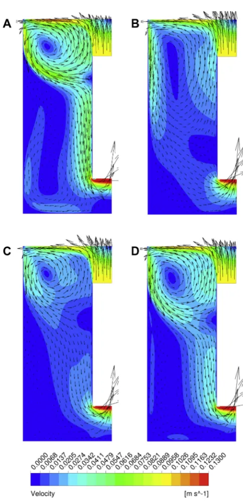
N1 480 960 160200 0.37 Figure 3.2.Velocity contour and vector plots for k-xSST (A), RNG k-(B), Linear

[image:5.595.42.293.700.754.2]

(6)

3.2. Turbulence model comparison

In order to choose the most appropriate turbulence model for the flow in this gas-lift digester, the applicability of the turbulence models available was assessed based on the flow characteristics that needed to be captured. As was stated previously the flow sep-aration from the outer wall is important to the overall flow pattern in the digester and so needs to be accurately predicted. Therefore, the turbulence models applied were chosen based on their histor-ical ability to capture these flow features.Fig. 3.2shows contour and velocity plots of the flow fields for each of the turbulence mod-els implemented.Fig. 3.5(E) shows the respective experimental re-sults for the comparable setup and operating conditions as reported by Karim et al. (2004) which was used for validation purposes.

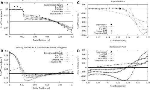
The axial velocity profiles produced by each simulation are compared to the experimental results of Karim et al. (2004) in Fig. 3.3(A) and (B) at 0.0325 and 0.1875 m from the bottom of the digester. The profiles predicted by all three turbulence models at the outlet are significantly different to those observed in exper-iment. This is likely due to the boundary condition applied (lower end of draft tube), the use of a pressure outlet with a gauge pres-sure of 0 Pa appears to be drawing the fluid through the lower end of the draft tube significantly faster than the experimental work indicates should be happening. This indicates the need for more detailed modelling of the outlet boundary condition if the singlephase approximation is to be used. The numerical solutions for the profile at the top of the draft tube are much more in line with the experimental; the velocity profile at the top of the draft tube however is constant in the modelled solutions where the experimental work shows a varied profile which is in keeping with the bubble flow. The effect of this profile shape would require more

testing to determine its effect on the solution in the main annular section. This is likely to only have noticeable qualitative effect on the ﬂow pattern in the area directly above the draft tube and not alter the solution in the main annular section signiﬁcantly. The comparison between the multiphase and singlephase shown in Section 3.4 gives some preliminary evidence to support this.

A comparison between the separation and reattachment points for each of the turbulence models shows a more significant varia-tion than for the axial velocity profiles (Fig. 3.3(C) and (D)). It is much more obvious that the Linear RSM and Transition SST models better predict the points at which the flow separates and reat-taches at the wall. The RNG k-

model under predicts the separa-tion and reattachment points most obviously with a signiﬁcant delay in the separation location. This inability to predict separation point is a known issue with

e

based turbulence models (Menter, 1993). Conversely the k-

x

SST model predicts the separation point too early.

[image:6.595.43.545.430.732.2]

The use of a turbulence model that is capable of predicting large streamline curvature, boundary layer separation and Laminar-Turbulent transition is necessary to accurately capture the flow features of this digester. Of the turbulence models applied the re-sults that appear to most closely follow the experimental rere-sults ofKarim et al. (2004)are those of the Linear RSM and Transition SST models (Fig. 3.2(C) and (D) respectively). Both models seem to give a similar result for the separation and reattachment points as well as the velocity profiles near the inlet and outlet. Both also manage to pick up the stagnation zone, although the RSM model appears to have less recirculation in the region than the Transition SST. The RNG and SST models however, significantly over or under predict the point at which the separation and reattachment occurs having and adverse effect on the prediction of the stagnation re-gion and giving rise to higher velocities near the draft tube wall;

Figure 3.3.Axial velocity proﬁles at 0.1875 m (A) and 0.0325 m (B) from base of digester for different turbulence models compared with experimental results obtained by

(7)

thus, more recirculation is seen in the stagnation zone. Overall there is significant difference in the flow patterns of the digester for each of the results showing how significant the choice of turbu-lence model is to the accuracy of the solution. The two-equation

[image:7.595.83.519.86.236.2]

models showed poor results when compared to the experimental data, particularly with regard to the ﬂow separation. The two more computationally expensive models showed signiﬁcant improve-ment in this region and in capturing the stagnation zone. This Table 3.2

Fluent and OpenFOAM settings comparison.

Setting Fluent 13.0sp2 OpenFOAM-2.0.1

Solver Coupled Simple

Turbulence model k-xSST k-xSST Wall treatment Blended VSM Blended VSM

Boundary conditions

Inlet Velocity normal inlet 0.09804 ms1

Velocity normal inlet 0.09804 ms1

Outlet 0 Pa gauge pressure 0 Pa ﬁxed value

Walls No slip No slip

Surface Zero shear Zero shear

Discretization schemes

Gradient scheme Least squares cell based Least squares Pressure second order Least squares

Momentum Third order MUSCL r:Gauss MUSCL,r2_{:Gauss Linear Corrected}

Turbulent kinetic energy (k) Third order MUSCL r:Gauss MUSCL,r2

:Gauss Linear Corrected Speciﬁc dissipation rate (x) Third order MUSCL r:Gauss MUSCL,r2

:Gauss Linear Corrected

[image:7.595.55.552.270.682.2]

(8)

indicates that for digesters that are of a similar type where transi-tional flow is likely to occur or flow separation is possible the choice of turbulence model should be considered carefully. In cases where low Reynolds number flows are likely to be found (e.g. bench-scale and pilot-scale digesters) the use of two equation k-

models with standard wall functions is inappropriate and should be avoided. If due to computational expense a two equation model is preferred the k-

x

SST with blended wall treatment is rec-ommended or for flow with boundary layer separation the Transi-tion-SST model can be used to more accurately capture the separation location. More careful selection of a turbulence model when simulating mixing in anaerobic digesters particularly in bench scale digesters with low Reynolds number flow should help improve digester design predictions when these complex flow fields are involved. The prediction of flow separation has been shown to have a significant effect on the size of stagnation region and on the velocities in the digester. Accurate prediction of such features is important when designing digesters to perform reliably and efficiently.

3.3. Solver independence study

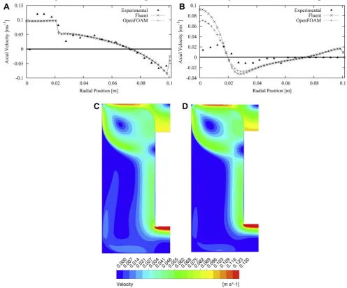
In order to be assured the results being obtained were solver independent a comparison between results from Fluent 13.0sp2 and OpenFOAM 2.0.1 was made.Table 3.2shows the settings used in both the solvers including boundary conditions and discretiza-tion schemes.

OpenFOAM is an open source CFD code and like Fluent it is Fi-nite Volume based. It would be expected that both solvers should produce very similar results when using the same (in principal) settings. The k-

x

SST turbulence model was used as its application and the near wall treatment available in OpenFOAM is produced from the work ofMenter and Esch (2001)as in Fluent. The avail-ability of the VSM for near wall treatment when using the k-

x

SST in OpenFOAM allows the solver settings to be kept as similar as possible to those used in Fluent.Fig. 3.4(C) and (D) shows con-tours of velocity magnitude for the two solvers, as can be seen there is qualitatively little difference in the solutions in regards to the general flow field. However, the velocity profiles shown in Fig. 3.4(A) and (B) do highlight some very minor differences. The profiles at 0.1875 m show little difference, whereas the solution at 0.0325 m shows a slight divergence between the results below the outlet. This is likely due to the formulation of the pressure out-let boundary condition being different in the two solvers. This strong agreement of the two solvers confirms that the study results are solver independent.

3.4. Euler–Lagrange multiphase modelling

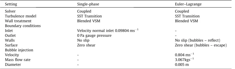
[image:8.595.51.543.366.723.2]

This section details the results obtained from the more complex multiphase modelling described in Section2.3when used to model the digester. The Euler–Lagrange method was used to assess the ef-fect of the assumptions made at the top and bottom of the draft tube in the singlephase model. Of particular interest is the effect

(9)

the different methods have on the area above and below the draft tube where the singlephase inlet and outlet conditions will have greatest influence.Table 3.3shows the solver settings for the mul-tiphase model compared to the singlephase setup used previously. In order to keep the model as simple as possible without unduly affecting the solution several assumptions were made with regard to the bubbles. The first assumption was to release the bubble half way between the draft tube wall and the gas inlet pipe (location 0.011, 0.04). This allows the bubble to rise unhindered by the walls which would not be the case if the bubbles were released from the bottom of the gas inlet pipe. By injecting the bubbles in this way the inclusion of thin film models for the walls is unnecessary as the bubbles rise without coming into contact with the walls. Axi-symmetry was also assumed as with the singlephase model, which for the Lagrangian phase results in a continuous bubble ring.

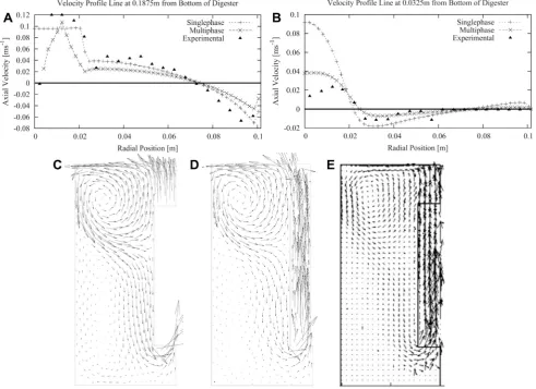
From the results of the singlephase model the turbulence model that produced the most satisfactory results was the SST Transition model, as such this was chosen for use in the multiphase models. Fig. 3.5shows the velocities for both models and experimental re-sults at the previously mentioned profile heights and for the full flow fields respectively. They illustrate that the results for the sin-glephase solution, with a calculated value for the slurry flow rate at the top of the draft tube, give a good approximation to the solution of the multiphase simulation. The calculated inlet however is a flat constant profile as opposed to the varied profile of the Euler– Lagrange model. This has some effect on the velocity of the solu-tions and particularly on the solution between the top of the draft tube and the slurry surface. It may be possible to approximate this using a non-uniform inlet profile at the inlet. The other main differ-ence between the Euler–Lagrange and singlephase solutions is at the bottom of the draft tube. It can be seen fromFig. 3.4(B) that the solution for the singlephase has an average velocity at the draft tube outlet more than twice that of the Euler–Lagrange model. This is likely due to the outlet boundary condition used in the single-phase model. The 0 Pa pressure outlet is likely causing the fluid to be drawn out in an artificial manner not found in the real digester.

The vector plots inFig. 3.4(C)–(E) show that both the single-phase and multisingle-phase solutions give good approximations to the experimental results. However, the ﬂow ﬁeld for the multiphase solution appears to give a slightly better approximation for the stagnation region and at the bottom of the draft tube. This is due to the locally high velocities produced by the pressure drop at the 0 Pa pressure outlet boundary condition used in the single-phase model.

With results of the multiphase model being comparable to those of the singlephase solution a degree of conﬁdence in using singlephase models for this type of digester is appropriate. Such a reduction in model complexity without signiﬁcant change in re-sults is a desirable feature in a CFD model. The reduction in com-putational expense is important in reducing the design

turnaround time and will help in the development of more efﬁcient digesters of this type.

4. Conclusions

This numerical study into the effects of turbulence model selec-tion for ﬂow predicselec-tions in a gas-lift anaerobic digester concludes:

The Transition-SST turbulence model provides the most accu-rate predictions for velocity, separation/reattachment and over-all ﬂow-ﬁeld.

The RNG k-

model is shown to be unsuitable for modelling the low-Renumber ﬂows found in the model digester and signiﬁ-cantly under predicts separation/reattachment points and the size of stagnation regions.

The k-

x

SST and RSM provide more accurate results; however exhibit some inaccuracies with velocity and separation/reat-tachment prediction.

Euler–Lagrange multiphase and singlephase predictions provide comparable solutions in the main reactor.

Acknowledgements

This research was partially funded by the EPSRC (Engineering and Physical Sciences Research Council).

References

Aubin, J., Fletcher, D.F., Xuereb, C., 2004. Modeling turbulent ﬂow in stirred tanks with CFD: the inﬂuence of the modeling approach, turbulence model and numerical scheme. Experimental, Thermal and Fluid Science 28, 431–445.

Blazek, J., 2005. Computational Fluid Dynamics: Principles and Applications, second ed. Elsevier.

Brebbia, C.A., Mammol, A.A., 2011. Computational Methods in Multiphase Flow VI.

Bridgeman, J., 2012. Computational ﬂuid dynamics modelling of sewage sludge mixing in an anaerobic digester. Advances in Engineering Software 44, 54–62.

Celik, I.B., Ghia, U., Roache, P.J., Freitas, C.J., Coleman, H., Raad, P.E., 2008. Procedure for estimation and reporting of uncertainty due to discretization in CFD applications. Journal of Fluids Engineering 130.

Joshi, J.B., Nere, N.K., Rane, C.V., Murthy, B.N., Mathpati, C.S., Patwardhan, A.W., Ranade, V.V., 2011. CFD simulation of stirred tanks: comparison of turbulence models. Part I: Radial ﬂow impellers. The Canadian Journal of Chemical Engineering 89, 23–82.

Karim, K., Thoma, G.J., Al-Dahhan, M., 2007. Gas-lift digester conﬁguration effects on mixing effectiveness. Water Research 41, 3051–3060.

Karim, K., Varma, R., Vesvikar, M., Al-Dahhan, M., 2004. Flow pattern visualization of a simulated digester. Water Research 38, 3659–3670.

Kojima, H., Sawai, J., Uchino, H., Ichige, T., 1999. Liquid circulation and critical gas velocity in slurry bubble column with short size draft tube. Chemical Engineering Science 54, 5181–5185.

Menter, F.R., 1993. Zonal two equation k-w turbulence models for aerodynamic ﬂows. In: AIAA Paper 93-2906, 24th Fluid Dynamics Conference, July 6–9, Orlando, Florida, USA, p. 21.

Menter, F.R., 2011. Turbulence Modeling for Engineering Flows. ANSYS Inc. (Technical Paper 25).

[image:9.595.99.512.86.208.2]

Menter, F.R., Esch, T., 2001. Elements of industrial heat transfer prediction. In: 16th Brazilian Congress of Mechanical Engineering (COBEM).

Table 3.3

Comparison of solver settings for singlephase and multiphase models.

Setting Single-phase Euler–Lagrange

Solver Coupled Coupled

Turbulence model SST Transition SST Transition Wall treatment Blended VSM Blended VSM Boundary conditions

Inlet Velocity normal inlet 0.09804 ms1

-Outlet 0 Pa gauge pressure

-Walls No slip No slip (bubbles – reﬂect) Surface Zero shear Zero shear (bubbles – escape) Bubble injection

Velocity - 0.804 ms1

Mass ﬂow rate - 3.067kgs1

(10)

Menter, F.R., Kuntz, M., Langtry, R., 2003. Ten years of industrial experience with the SST turbulence model. In: Hanjalic, K., Nagano, Y., Tummers, M. (Eds.), Proceedings of the Fourth International Symposium on Turbulence, Heat and Mass Transfer, Antalya, Turkey.

Menter, F.R., Langtry, R.B., Likki, S.R., Suzen, Y.B., Huang, P.G., Völker, S., 2006. A correlation-based transition model using local variables—Part I: Model formulation. Journal of Turbomachinery 128, 413.

Meroney, R.N., 2009. CFD simulation of mechanical draft tube mixing in anaerobic digester tanks. Water Research 43, 1040–1050.

Mudde, R.F., Van Den Akker, H.E.A., 2001. 2D and 3D simulations of an internal airlift loop reactor on the basis of a two-ﬂuid model. Chemical Engineering Science 56, 6351–6358.

Oey, R.S., Mudde, R.F., Van Den Akker, H.E.A., 2003. Numerical simulations of an oscillating internal-loop airlift reactor. The Canadian Journal of Chemical Engineering 81, 684–691.

Sieblist, C. Lübbert, A. 2010. Gas Holdup in Bioreactors. Encyclopedia of Industrial Biotechnology: Bioprocess, Bioseparation, and Cell Technology. John Wiley & Sons, Inc., pp. 1–8.

Taricska, J.R., Long, D.A., Chen, P., Hung, Y.-T., Zou, S.-W., 2009. Anaerobic Digestion, in: Biological Treatment Processes - Handbook of Environmental Engineering. vols. 8. Springer, pp. 589–634.

Terashima, M., Goel, R., Komatsu, K., Yasui, H., Takahashi, H., Li, Y.Y., Noike, T., 2009. Bioresource technology CFD simulation of mixing in anaerobic digesters. Bioresource Technology 100, 2228–2233.

Turovskiy, I.S., Mathai, P.K., 2006. Wastewater Sludge Processing. John Wiley & Sons, Inc., New Jersey.

Vesvikar, M.S., Al-Dahhan, M., 2005. Flow pattern visualization in a mimic anaerobic digester using CFD. Biotechnology and Bioengineering 89, 719–732.

Wu, B., 2010a. CFD simulation of mixing in egg-shaped anaerobic digesters. Water Research 44, 1507–1519.

Wu, B., 2010b. CFD simulation of gas and non-Newtonian ﬂuid two-phase ﬂow in anaerobic digesters. Water Research 44, 3861–3874.

Wu, B., 2011. CFD investigation of turbulence models for mechanical agitation of non-Newtonian ﬂuids in anaerobic digesters. Water Research 45, 2082–2094.

Wu, B., Chen, S., 2008. CFD simulation of Non-Newtonian ﬂuid ﬂow in anaerobic digesters. Biotechnology and Bioengineering 99, 700–711.