This is a repository copy of A comparison of methods for converting DCE values onto the
full health-dead QALY scale.
White Rose Research Online URL for this paper:
http://eprints.whiterose.ac.uk/74892/
Article:
Rowen, Donna, Brazier, John and Hout, Ben, Van (2011) A comparison of methods for
converting DCE values onto the full health-dead QALY scale. HEDS Discussion Paper
11/15. (Unpublished)
[email protected] https://eprints.whiterose.ac.uk/ Reuse
Unless indicated otherwise, fulltext items are protected by copyright with all rights reserved. The copyright exception in section 29 of the Copyright, Designs and Patents Act 1988 allows the making of a single copy solely for the purpose of non-commercial research or private study within the limits of fair dealing. The publisher or other rights-holder may allow further reproduction and re-use of this version - refer to the White Rose Research Online record for this item. Where records identify the publisher as the copyright holder, users can verify any specific terms of use on the publisher’s website.
Takedown
If you consider content in White Rose Research Online to be in breach of UK law, please notify us by
- 1 -
HEDS Discussion Paper
11/15
A comparison of methods for converting DCE values
onto the full health-dead QALY scale
Donna Rowena, John Braziera, Ben Van Houta
Disclaimer:
This series is intended to promote discussion and to provide information about work in progress. The views expressed in this series are those of the authors, and should not be quoted without their permission. Comments are welcome, and should be sent to the corresponding author.
White Rose Repository URL for this paper: http://eprints.whiterose.ac.uk/74892
A comparison of methods for converting DCE values onto
the full health-dead QALY scale
Donna Rowena, John Braziera, Ben Van Houta
a
School of Health and Related Research (ScHARR), University of Sheffield
* Correspondence to: Donna Rowen, Health Economics and Decision Science, University of Sheffield, Regent Court, 30 Regent Street, Sheffield, S1 4DA, UK.
Telephone: +44114 222 0728. Fax: +44114 272 4095.
Email: [email protected]
Key words: Preference-based measures of health; quality of life; Discrete Choice
Experiment; Pairwise comparisons
Funding source: Data collection was funded by Novartis.
1
A comparison of methods for converting DCE values onto
the full health-dead QALY scale
Abstract
Cardinal preference elicitation techniques such as time trade-off (TTO) and Standard
Gamble (SG) receive criticism for their complexity and difficulties in using them in more
vulnerable populations. Ordinal techniques such as discrete choice experiment (DCE) and
Best Worst Scaling (BWS) are easier, but values generated by them are not anchored onto
the full health-dead 1-0 QALY scale required for use in economic evaluation. This paper
explores new methods for converting modelled DCE latent values onto the full health-dead
QALY scale: (1) anchoring assuming worst state is equal to being dead; (2) anchoring DCE
values using dead as valued in the DCE; (3) anchoring DCE values using TTO value for
worst state; (4) mapping DCE values onto TTO; (5) combining DCE and TTO data in a
hybrid model. We use postal DCE data (n=263) and TTO data (n=307) collected by interview
in a general population valuation study of an asthma condition-specific measure (AQL-5D).
Methods (4) and (5) using mapping and hybrid models perform best; the anchor-based
methods perform relatively poorly. These new methods have a useful role for producing
values on the QALY scale from ordinal techniques such as DCE and BWS for use in cost
2
INTRODUCTION
Economic evaluation measuring outcomes using quality-adjusted life years (QALYs) has
increasingly informed resource allocation in recent years. The QALY is a measure of health
outcome that combines quality of life with length of life. Quality of life is measured on a full
health-dead 1-0 scale, where one equals full health and zero is equal to being dead, with
negative values where quality of life is regarded as worse than being dead. For the complex
decision problems faced by agencies such as the National Institute for Health and Clinical
Excellence (NICE) this has been extremely useful for informing decision making of resource
allocation for health care programmes using incremental cost per QALY analyses. The
QALY enables comparisons across interventions that impact on mortality, morbidity and
both. These comparisons cannot be avoided, and the QALY provides a useful summary
measure that enables the full rigours of modern cost effectiveness analysis to be applied.
However there remains much debate surrounding the elicitation of utilities to produce the ‘Q’ quality adjustment weight of the QALY.
Standard cardinal techniques for eliciting preferences for health states have been time
trade-off (TTO), standard gamble (SG) TTO, SG and visual analogue scale (VAS). There has been
much debate in the literature regarding the best technique. TTO and SG have been
regarded by many as superior to VAS for eliciting preferences since they are based on
choices that involve sacrificing (i.e. some notion of opportunity costs), although there is often
little agreement in values elicited using these two techniques. On the other hand, SG and
TTO have been criticised for being too complex for many respondents and effectively
disenfranchising important groups in society such as the very elderly and the young, and
some cultures. This has led to increasing interest in the use of ordinal techniques, such as
pairwise discrete choice experiment (DCE) where respondents choose between two health
states and best-worst scaling (BWS) where respondents choose the best and worst
attributes of a health state, including application of BWS to measures of capabilities (Coast
et al. 2008) and social care outcomes (Netten et al. 2012).
DCE has been used for eliciting utility values for different health care programmes, but has
had limited use for eliciting utility values for health states to inform the scoring systems for
preference-based measures of health. A small number of studies have used DCE to value
health states (Brazier et al. 2011;Burr et al. 2007;Hakim and Pathak 1999;Osman et al.
2001;Ratcliffe et al. 2009;Ryan et al. 2006) but the majority of these have not anchored
values on the full health-dead QALY scale. DCE values can be modelled using regression
3
severity level of each dimension in the classification system, but these coefficients are
expressed on a modelled latent utility value that has arbitrary anchors. Some studies anchor
values onto a 1-0 best state-worst state scale (Burr, Kilonzo, Vale, & Ryan 2007;Ryan,
Netten, Skatun, & Smith 2006) but this is an arbitrary assumption dependent on the specific
dimensions and severity levels included in the classification system. Three published DCE
studies have attempted to anchor the modelled latent utility values onto the full-health QALY
scale. The first study anchors modelled DCE values using the TTO value for the worst health
state defined by the classification system (Ratcliffe, Brazier, Tsuchiya, Symonds, & Brown
2009). This represents a rather crude attempt to anchor DCE values onto a full health-dead
scale using just one data point. The second study incorporates a dead state into pair wise
DCE tasks and estimates an additive regression model that includes a dummy variable for
dead (Brazier, Rowen, Tsuchiya, & Yang 2011). The regression coefficients are normalised
onto the full health-dead scale by dividing the coefficient on each level by the coefficient on
the dead dummy variable. This method has been criticised (Flynn et al. 2008) as many
respondents do not see any states described by the classification system as worse than
being dead. While the proportion who do regard any state as worse than dead is as small as
15% in the case of EQ-5D, it is usually higher than this (e.g. 66% for SF-6D) and for these
respondents the appropriateness of this method is questioned. The third study incorporated
duration into the DCE task. This presents design and modelling challenges that have been
addressed (Bansback et al. 2010), since the relationship between quality of life and survival
is not additive. However, the incorporation of duration into the DCE task increases the
complexity of the task, and does not offer a solution to the increasingly used BWS technique.
This paper explores these methods for anchoring DCE and BWS values onto the full
health-dead QALY scale and two new ones. It uses a data set from a general population valuation
study of an asthma condition-specific measure (AQL-5D) using TTO and DCE. Alternative
methods for anchoring the DCE data onto the full health-dead scale are explored: (1)
anchoring assuming worst state is equal to being dead; (2) anchoring the modelled DCE
latent variable using dead as valued in the DCE; (3) anchoring the modelled DCE latent
variable using the TTO value for the worst state; (4) mapping the modelled DCE latent
variable onto TTO; (5) combining DCE and a sample of TTO data in a hybrid model. The
comparison of methods will inform researchers about the relative merits of using each
4
METHODS
Health state description
Health states are described using an asthma-specific preference-based measure, AQL-5D,
(Young et al. 2011) derived from the Asthma Quality of Life Questionnaire, AQLQ (Juniper
EF et al. 1993). AQL-5D has 5 dimensions: concern about asthma, shortness of breath,
weather and pollution stimuli, sleep impact and activity limitations each with 5 levels of
severity to define a total of 3125 health states (see Table 1).
Valuation surveys
Interview
Interviews were undertaken to elicit health state utility values for a selection of AQL-5D
states using TTO from a representative sample of the general population. Respondents were
interviewed in their own home by trained and experienced interviewers. At the start of the
interview respondents were informed about asthma using an information sheet. To
familiarise respondents with the system respondents who had asthma were asked to
complete the health state classification system for themselves; respondents who did not
have asthma were asked to complete the health state classification system for someone
they knew who had asthma or to imagine somebody with asthma. Respondents were then
asked to rank 7 intermediate states, full health (health state 11111), worst state defined by
the health state classification (health state 55555), and immediate death.
Respondents then valued a practice state using TTO, and this was followed by valuation of
the 7 intermediate states and the worst state using TTO, with an upper anchor of full health
(health state 11111). The survey used the used the Measurement and Valuation of Health
(MVH) study version of TTO, including a visual prop designed by the MVH group (University
of York) (Dolan 1997;Gudex 1994). Respondents were then asked questions about their
socio-economic characteristics and health service use, how difficult they found the rank and
TTO tasks and finally whether they were willing to participate in a postal survey (described
below).
The classification system describes too many states for valuation, and a sample of states
were selected for valuation using TTO using the specification of a regression model
estimated on TTO data to estimate preference weights for all severity levels of each
dimension in the classification system, using level 1 as the baseline. Health states were
selected using a balanced design, which ensured that every level of every dimension had an
5
design selected 98 health states which were then randomly stratified into mixed severity
groups of 7 states based on their summed severity score (summing the scores on all 5
dimensions e.g. 22222 has a severity score of 10). These combinations of 7 states made up
the card blocks used in the interviews, to ensure each intermediate state was valued an
equal number of times and that respondents valued states with a wide range of severity. The
worst state is valued by all respondents to increase accuracy for this value and enable
responses to be compared across groups of respondents valuing different intermediate
states.
Postal survey
Interviewees who had stated in the interview that they were willing to complete a postal
survey were mailed a postal DCE questionnaire approximately four weeks after the
interviews. The questionnaire was also mailed to a sample of the general public who had not
been previously interviewed. At the start of the survey respondents were asked to complete
the health state classification system for themselves to help familiarise them with the
classification. Respondents were then asked a practice pairwise comparison question
followed by a series of 8 pairwise comparisons, where for each comparison respondents
were asked to indicate which health state they preferred. Finally respondents were asked
questions about their socio-demographic characteristics. Reminders were sent to all
non-responders approximately four weeks after the initial questionnaire was sent.
Combinations of health states for the pairwise comparisons were selected using the
D-efficiency approach using a specially developed programme (Huber and Zweina 1996) in
statistical software SAS. The programme obtained an optimal statistical design based on
level balance, orthogonality, minimal overlap and utility balance which reduced the number
of pairwise comparisons required for valuation. The programme selected 24 pairwise
comparisons which were randomly allocated to four questionnaire versions each with 6
comparisons. Each questionnaire also included two identical pairwise comparisons
comparing a severe health state (state 44355) and the worst health state to ‘immediate
death’.
Modelling health state values
Time trade-off
TTO data was analysed using a one-way error components random effects model via
generalised least squares (GLS). This takes account of the structure of the data as each
6
ij i ij f
U (X )
(1)Where Uijrepresents TTO disvalue (1–TTO value) for health state i=1,2 …n valued by respondent j=1,2…m, Xi represents a vector of dummy variables for each level of
dimension ∂ of the health state classification system where level = 1 is the baseline for
each dimension and
ij is the error term. The error term is subdivided
ij ujeij, where ujis the individual random effect and eij is the usual random error term for the ith health state
valuation of the jth individual. Other models estimated using this data are reported elsewhere (Yang et al. 2011).
DCE and TTO
DCE data was modelled to produce cardinal utility estimates on a latent utility scale. The
DCE data was modelled using a random effects probit model which takes account of the
structure of the data where each respondent valued multiple states, using an additive
specification as outlined in equation (1) (Ratcliffe, Brazier, Tsuchiya, Symonds, & Brown
2009). This model produced coefficients on a latent utility scale with arbitrary anchors. This
model excluded data collected for the pairwise comparisons involving the state ‘dead’.
Translating DCE scores onto the full health-dead scale
Method (1): anchoring using worst state equals zero
The coefficients from the Probit model were normalised using
5
r where r
is the rescaled coefficient for level of dimension ∂, is the coefficient for level of
dimension ∂, and 5is the coefficient for the worst level (level 5) of dimension ∂. The coefficients for the worst level of each dimension sum to -1. This method produces utility
estimates for all health states anchored on a 1-0 best state-worst state scale.
Method (2): anchoring using the coefficient for ‘dead’
Firstly all DCE data including data for the pairwise comparisons involving the state ‘dead’
was modelled using a random effects probit model (Brazier, Rowen, Tsuchiya, & Yang
2011). The model specification was:
ij
ij
f
D
7
Where Uijrepresents utility for health state i=1,2 …n valued by respondent j=1,2…m, Xi
represents a vector of dummy variables for each level of dimension ∂ of the health state
classification system, Drepresents a dummy variable for the state ‘dead’ and
ij is the error term. Secondly coefficients for each level of each dimension were normalised by dividing bythe dead dummy variable;
r where r is the rescaled coefficient for level of dimension ∂, is the coefficient for level of dimension ∂ and is the coefficient for the dead dummy variable (see (Brazier, Rowen, Tsuchiya, & Yang 2011) for use of this
technique in DCE data and (McCabe et al. 2006;Salomon 2003) for use of this technique in
rank data).
Method (3): anchoring the worst state using TTO
The coefficients on a latent utility scale estimated in the first stage of method (1) were
normalised onto the full health-dead scale using the estimated TTO value of the worst state.
This means that the value of the worst state in the DCE model is anchored at the TTO value
of the worst state.
Method (4): mapping DCE onto TTO
Mapping is a method often used to estimate utility values for a trial (or study) when a utility
measure was not included in the trial. This is achieved by predicting utility values for the trial
using the statistical relationship between data included in the trial and the preferred utility
measure (see (Brazier et al. 2010) for a recent review of mapping). This mapping principle
was used here to estimate TTO values for all states using modelled latent DCE values for all
states. By using more than one health state TTO value it should provide a more accurate
method.
The probit model estimated on DCE data generates values on a latent utility scale for all
3125 states. Ninety-nine of these states have mean TTO values collected in the interviews.
The simple mapping function from TTO to DCE was specified as:
i i
i f DCE
TTO ( )
(3)Where TTOi represents mean TTO value of health state i, DCE represents the modelled
latent utility value for health state i and
i is the error term. The first specification assumes alinear relationship with an intercept, and then squared and cubic terms were added to see
8
The interest in this method is in the use of a small TTO study accompanying a larger DCE
survey. One issue is the selection of the potential size of such a TTO survey and so this
study examines the valuation of 10, 19 and 99 states. Method (4a) used 10 health states
selected by ordering latent DCE utility estimates by severity (using the modelled DCE latent
estimate) from mildest to most severe and selecting the states valued 1st, 11th, 22nd, 33rd,
44th, 55th, 66th, 77th, 88th and 99th. Method (4b) used 19 states, the states used in method 4a
were supplemented by states valued 6th, 16th, 27th, 38th, 49th, 60th, 71st, 82nd and 93rd. The
rationale for choosing 10 and 19 states was logistical; these states can be easily valued by
respondents using TTO. The study design for method (4a) requires respondents to value all
10 states using TTO; study design for method (4b) requires respondents to value 10 states,
consisting of 9 states plus the worst state using two different card blocs in the interviews.
More and different states could have been chosen, but these were selected to provide an
indication of how the method performs. Method (4c) used all 99 states in order to examine
the degree of improvement from increasing the number of states valued by TTO up to the
number required to estimate a well specified TTO algorithm.
Method (5): hybrid models
This method combines TTO data with discrete choice data using both a likelihood approach
and a Bayesian approach. The idea behind both approaches has an analogy to survival data
where data are combined on patients who died and patients who have not; patients who
have died offer exact information, and patients who have not yet died offer censored
information. By analogy TTO data give exact information about the utility of a health state
and discrete choice data offer censored data that indicates whether the value of one state is
higher than the value of another state but not the degree to which it is higher. As with
survival analyses, these two sources of data can be brought together using a single
likelihood-function. Methods (5a), (5b) and (5c) use individual level TTO data for the states
selected in method (4) and all DCE data. Technical details are presented in the Appendix.
Comparison of models
The most important aspect of model performance is accuracy of the estimated utility values
anchored onto the full health-dead scale as indicated by the mean observed TTO health
state values. . Model performance was assessed using mean absolute difference between
observed TTO and predicted health state utility values (MAD) at the health state level, root
9
is greater than 0.05 and 0.1 respectively. Predictions from the 5 methods (and their
variations) were plotted alongside mean observed values for the 99 states valued by TTO.
RESULTS
The data
The TTO dataset contains 307 successfully conducted interviews, providing a response rate
of 40% for suitable respondents answering their door at time of interview. Each intermediate
health state was valued 19 to 22 times, and the worst state was valued 307 times. The
distribution of TTO values was negatively skewed and mean TTO value for the 99 health
states ranged from 0.39 to 0.94. Further details are reported elsewhere (Yang, Brazier,
Tsuchiya, & Young 2011).
The DCE dataset contains 263 successfully completed postal surveys. Out of the 307
respondents who were interviewed 168 returned postal DCE questionnaires (55%). Out of
the 400 households receiving the postal questionnaire who were not previously interviewed
95 returned questionnaires (24% return rate). Data from all respondents have been pooled
since previous analyses showed no significant difference between them (Brazier, Rowen,
Tsuchiya, & Yang 2011).
Table 2 reports the socio-demographic composition of the TTO and DCE samples. Both
samples are similar, but the TTO sample is younger and healthier, with a higher proportion
of males. Self-reported health status using EQ-5D (Dolan 1997) was similar for each sample
to the UK EQ-5D norms of 0.85 for females and 0.86 for males (Kind et al. 1999).
TTO model
Table 3 reports the model estimated on TTO data. The majority of coefficients were negative
and the size of coefficients were consistent, where more severe levels of each dimension
had a larger utility decrement. Three coefficients were positive but small and statistically
insignificant.
DCE model
The DCE model producing latent DCE estimates that are unanchored onto a full health-dead
1-0 scale is reported in Table 3. Estimated coefficients for both methods had four
inconsistencies, level 2 of concern, breathlessness and pollution and level 3 of pollution,
10
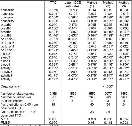
Methods (1) to (3): anchoring
Results for methods (1) and (3) anchor the latent DCE estimates, and have the same
inconsistent coefficients as the latent estimates for level 2 of concern, breathlessness and
pollution and level 3 of pollution (Table 3). Method (1) anchored coefficients of the DCE
model by dividing them by the coefficient for the worst state and method (3) anchored
coefficients of the DCE model by dividing them by TTO value for the worst state. Method (2)
modelled all DCE data including comparisons involving the ‘dead’ state and anchored coefficients using the coefficient for ‘dead’. This method had three of the four positive coefficients of the latent DCE estimates, and the same coefficient (level 2) was significant.
All 3 methods anchored the DCE data similarly and the pattern of the coefficients was
similar. The most noticeable differences were at the lower end of the dimensions for
concern, short of breath, sleep and activities where methods (2) and (1) in particular
produced larger coefficients than method (3) and the TTO model.
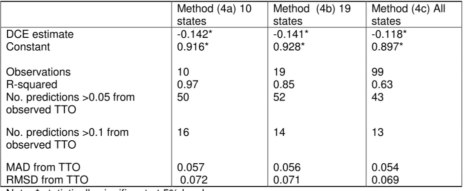
Method 4: mapping
Results for method (4) are reported in Table 4. The DCE coefficient is negative and
significant across all 3 models. The size of the intercept and the gradient associated with the
latent DCE value are similar across models using TTO data collected for 10, 19 and 99
health states (models (4a), (4b) and (4c) respectively). Plots of TTO and DCE data indicated
a linear relationship. The inclusion of squared and cubic terms were explored but these
variables were insignificant and did not improve model performance.
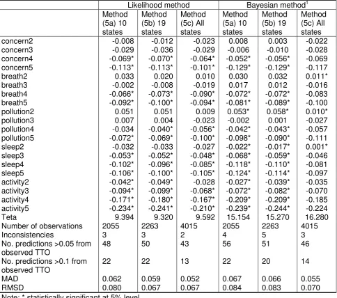
Method 5: hybrid models
Results for method (5) are reported in Table 5. All models for method (5) have been
estimated using both a common likelihood function and a Bayesian method. Overall the
coefficients are similar to the TTO model reported in Table 3. Coefficients were larger for
sleep and activity level 5 than in the TTO model, as also found for the anchor based models.
There was a tendency for the coefficients to move in the direction of the anchor based
models with larger coefficients for concern, sleep and activity levels 5, but this was less
marked and was not the case for breathing. This tendency was greater for the two models
with sub-samples of TTO valued states. For the likelihood model estimates using TTO data
for 10 and 19 states alongside all DCE data there are 3 consistencies, though none are
significant. The comparable models estimated using the Bayesian method have 4 and 5
11
Comparison of methods
The smallest difference between predicted values and observed mean TTO health state
values measured using MAD and RMSD were, as expected, the model estimated on a
dataset containing all TTO data, namely the TTO only model (MAD=0.056, RMSD=0.070).
This was followed by method (4c) mapping function (MAD=0.054, RMSD=0.069) and
method (5c) hybrid model estimated via the likelihood method using all 99 mean TTO health
state values (MAD=0.052, RMSD=0.067). Simple mapping functions using 10 and 19 mean
TTO health state values almost performed as well (MAD=0.057, RMSD=0.072 and MAD
0.056, RMSD=0.071 respectively). Hybrid models estimated using TTO values for 10 and 19
states also performed well with models estimated using the likelihood method (MAD=0.062,
RMSD=0.080 and MAD=0.059, RMSD=0.067) outperforming models estimated using the
Bayesian method (MAD=0.067, RMSD=0.084 and MAD=0.066, RMSD=0.083). The
mapping (4) and hybrid (5) methods had better model performance than the anchor based
methods. Method (3) was the best of the anchor models (MAD=0.075, RMSD=0.093),
followed by method (2) (MAD=0.093, RMSD=0.118) then method (1) (MAD=0.129,
RMSD=0.161).
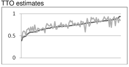
These differences in model performance are demonstrated in Figure 1. Method (4) produced
the utility estimates that best follow the pattern of observed TTO values. Method (1)
consistently under-estimated TTO values, but technically was anchored on a different scale
to TTO. Method (2) had more accurate estimates at the upper end of the scale but
under-estimation at the lower end of the scale. Method (3) over-estimated the value of most states.
Method (5) over-estimated values for the majority of health states, but perhaps to a less
severe extent than method (3).
DISCUSSION
This paper explored new methods for converting modelled DCE and BWS latent values for a
health state classification system onto the full health-dead 1-0 QALY scale and compared
these to methods used in the literature. The first new method mapped modelled DCE latent
values onto TTO values. The second method estimated utility decrements for each severity
level of the classification system by modelling DCE and TTO data together using a hybrid
model. These new methods produce utility estimates that are more similar to TTO estimates
than existing methods, and are more appropriate for anchoring DCE values onto the full
health-dead QALY scale. The analysis further explored whether these methods would
12
large DCE survey. Both methods produced relatively accurate predictions under these
circumstances.
These new methods potentially have a useful role in producing values on the QALY scale
using both ordinal DCE and cardinal TTO data that makes best use of the desirable
properties of each elicitation technique and elicited data. DCE has the advantage that it is a
cognitively simple task and values are not affected by time preference; but faces the
challenge of how to convert values onto the full health-dead scale. TTO encapsulates the
trade-off between quality and quantity of life; but can be cognitively demanding and data can
be expensive to collect. Combining these techniques may also mean that large scale data
collection using DCE can be undertaken inexpensively online, and small scale TTO data can
be collected by interview as its usability in an online environment is questionable. There has
also recently been interest in using DCE and BWS scaling to obtain values from children
(Ratcliffe et al. 2011) and elderly users of social care (Netten, Burge, Malley, Potoglou,
Towers, Brazier, Flynn, Forder, & Wall 2012).
Anchoring methods (1) to (3) used in the literature did not perform well compared to the new
approaches. Method (1) assumed that the worst state equalled zero and required no cardinal
data or pairwise comparisons involving the state ‘dead’, but had no empirical basis. Method (2) involved the use of pairwise comparisons with the state ‘dead’ and was an adaptation of a method successfully applied in rank data for several generic preference-based measures.
Using SF-6D and HUI2 data a regression model with the same specification as equation (2)
estimated on rank data was able to predict mean SG health state values reasonably well
(McCabe, Brazier, Gilks, Tsuchiya, Roberts, O'Hagan, & Stevens 2006). However when
using EQ-5D data the same model substantially over-predicted TTO health state values.
Model (2) estimated here replicated these results. The model has also been criticised since it
violates the assumptions of random utility theory for the large proportion of respondents who
do not value any state as worse than being dead (Flynn, Louviere, Marley, Coast, & Peters
2008). Method (3) anchored the DCE data using a single data point for the TTO value of
worst state. This method systematically over-estimated values due to its reliance on a single
TTO value.
Method (4) used a simple mapping based approach and achieved good predictions of
observed mean TTO health states values. Model performance was not largely affected when
the method was estimated using datasets containing TTO values for only 10 and 19 health
13
mean health state values. This would need further investigation before these results can be
used in economic evaluation, for example using bootstrapping methods to generate
confidence limits around these results.
Method (5) used a hybrid model to combine DCE and TTO data and had good model
performance. This method is more appealing statistically since it makes better use of the
data. Method (5) used individual level data whereas method (4) used mean level data,
meaning that method (5) does not suffer from problems associated with having only 10 or 19
data points. For this reason it is somewhat surprising that method (5) did not overwhelmingly
outperform model (4). The likelihood model performed better than the Bayesian method
across all samples. Further research using these hybrid models is recommended.
One key weakness is the study design of the DCE. The design used a limited number of pair
wise comparisons and was based upon the Huber and Zwerina design criteria which,
although widely used, do not guarantee optimal designs and on occasion cannot be used to
estimate all the main effects of interest (Huber & Zweina 1996). More sophisticated
approaches to DCE study design using optimal and near optimal designs are now being
recognised and applied in a health care context (Street and Burgess 2007;Viney et al. 2005).
It is impossible to completely rule out that the choice of DCE design may have impacted
upon the results achieved and further research is required to assess the replicability of the
comparative results found here in studies using optimal or near optimal DCE study designs.
However, a better DCE design is not likely to alter the results of the comparison of anchoring
methods, except that it may improve them all to some degree.
This study looked at DCE in the content of a condition-specific measure. One important
question is whether it would hold for BWS and for different classification systems. Research
recently completed developing and valuing a generic social care outcome measure (ASCOT)
with BWS has also found the mapping method to work well (though it has not been
compared to other methods (Netten, Burge, Malley, Potoglou, Towers, Brazier, Flynn,
Forder, & Wall 2012).
Ordinal methods such as discrete choice experiment (DCE) are a promising alternative for
valuing health state classification systems as they are cognitively easier than commonly
used cardinal methods of TTO and SG. However ordinal data has not been widely used to
date due to the challenge of anchoring ordinal data onto the 1-0 full health-dead QALY
14
health-dead QALY scale using mapping and estimation of a hybrid DCE and TTO model.
Both approaches required TTO data, but both performed well with TTO observations for only
10 health states. Anchor-based methods used in the literature performed poorly in
comparison to these methods. These new methods potentially have a useful role in
producing values on the QALY scale using both ordinal and cardinal data that makes best
15
Table 1 Classification system of asthma-specific measure AQL-5D
Concern
1. Feel concerned about having asthma none of the time
2. Feel concerned about having asthma a little or hardly any of the time 3. Feel concerned about having asthma some of the time
4. Feel concerned about having asthma most of the time 5. Feel concerned about having asthma all of the time
Short of breath
1. Feel short of breath as a result of asthma none of the time
2. Feel short of breath as a result of asthma a little or hardly any of the time 3. Feel short of breath as a result of asthma some of the time
4. Feel short of breath as a result of asthma most of the time 5. Feel short of breath as a result of asthma all of the time
Weather and pollution
1. Experience asthma symptoms as a result of air pollution none of the time
2. Experience asthma symptoms as a result of air pollution a little or hardly any of the time 3. Experience asthma symptoms as a result of air pollution some of the time
4. Experience asthma symptoms as a result of air pollution most of the time 5. Experience asthma symptoms as a result of air pollution all of the time
Sleep
1. Asthma interferes with getting a good night’s sleep none of the time
2. Asthma interferes with getting a good night’s sleep a little or hardly any of the time 3. Asthma interferes with getting a good night’s sleep some of the time
4. Asthma interferes with getting a good night’s sleep most of the time
5. Asthma interferes with getting a good night’s sleep all of the time
Activities
1. Overall, not at all limited with all the activities done 2. Overall, a little limitation with all the activities done
16
Table 2 Characteristics of respondents in valuation surveys
TTO interview sample (n=307) DCE postal survey (n=263) Age:
18-25 11.1% 3.4%
26-35 18.6% 13.3%
36-45 19.9% 17.1%
46-55 16.3% 21.3%
56-65 14.7% 24.3%
>66 19.5% 20.5%
Female 54.7% 56.3%
Self-reported EQ-5D scores:
17
Table 3 Anchor based methods (1) to (3) – TTO and normalised DCE model estimates
TTO Latent DCE estimates
Method (1)
Method (2)
Method (3)
concern2 -0.028 0.053 0.014 0.012 0.008
concern3 -0.044* -0.104 -0.027 -0.024 -0.015
concern4 -0.054* -0.394* -0.102* -0.099* -0.058*
concern5 -0.081* -0.649* -0.168* -0.139* -0.096*
breath2 0.000 0.173 0.045 0.025 0.025
breath3 -0.036* -0.017 -0.004 -0.008 -0.003
breath4 -0.101* -0.387* -0.100* -0.116* -0.057*
breath5 -0.116* -0.632* -0.164* -0.138* -0.093*
pollution2 -0.019 0.375* 0.097* 0.084* 0.055*
pollution3 -0.050* 0.067 0.017 -0.002 0.010
pollution4 -0.058* -0.153 -0.040 -0.051* -0.023
pollution5 -0.121* -0.427* -0.110* -0.085* -0.063*
sleep2 0.018 -0.182 -0.047 -0.022 -0.027
sleep3 0.010 -0.318* -0.082* -0.072* -0.047*
sleep4 -0.033* -0.636* -0.165* -0.125* -0.094*
sleep5 -0.054* -0.681* -0.176* -0.149* -0.100*
activity2 -0.039* -0.218* -0.056* -0.056* -0.032*
activity3 -0.059* -0.500* -0.129* -0.113* -0.074*
activity4 -0.175* -1.076* -0.278* -0.247* -0.158*
activity5 -0.197* -1.476* -0.382* -0.335* -0.217*
Dead dummy -1.000*
Number of observations 2456 1559 1559 2077 1559
Number of individuals 307 263 263 263 263
Inconsistencies 2 4 4 3 4
No. predictions >0.05 from observed TTO
19 40 34 24
No. predictions >0.1 from observed TTO
9 33 24 11
MAD 0.056 0.129 0.093 0.075
RMSD 0.070 0.161 0.118 0.093
18
Table 4 Method (4) - Mapping DCE onto TTO
Method (4a) 10 states
Method (4b) 19 states
Method (4c) All states
DCE estimate -0.142* -0.141* -0.118*
Constant 0.916* 0.928* 0.897*
Observations 10 19 99
R-squared 0.97 0.85 0.63
No. predictions >0.05 from observed TTO
50 52 43
No. predictions >0.1 from observed TTO
16 14 13
MAD from TTO 0.057 0.056 0.054
RMSD from TTO 0.072 0.071 0.069
19
Table 5 Method (5): DCE and TTO hybrid models
Likelihood method Bayesian method1
Method (5a) 10 states
Method (5b) 19 states
Method (5c) All states
Method (5a) 10 states
Method (5b) 19 states
Method (5c) All states
concern2 -0.008 -0.012 -0.023 0.008 0.003 -0.022
concern3 -0.029 -0.036 -0.029 -0.006 -0.010 -0.028
concern4 -0.069* -0.070* -0.064* -0.052* -0.056* -0.069
concern5 -0.113* -0.113* -0.101* -0.129* -0.129* -0.117
breath2 0.033 0.020 0.010 0.030 0.032 0.011*
breath3 -0.002 -0.008 -0.019 0.017 0.012 -0.016
breath4 -0.066* -0.073* -0.090* -0.072* -0.072* -0.083
breath5 -0.092* -0.100* -0.094* -0.081* -0.089* -0.100
pollution2 0.051 0.051 0.009 0.053* 0.058* 0.010*
pollution3 0.007 0.004 -0.023 -0.002 0.001 -0.027
pollution4 -0.034 -0.040* -0.056* -0.042* -0.043* -0.057
pollution5 -0.072* -0.069* -0.100* -0.098* -0.090* -0.111
sleep2 -0.032 -0.033 -0.027 -0.022* -0.017* 0.001*
sleep3 -0.053* -0.052* -0.048* -0.068* -0.059* -0.046
sleep4 -0.102* -0.096* -0.085* -0.118* -0.110* -0.081
sleep5 -0.106* -0.100* -0.105* -0.124* -0.114* -0.097
activity2 -0.042* -0.049* -0.028 -0.027* -0.039* -0.035
activity3 -0.094* -0.099* -0.068* -0.072* -0.082* -0.070
activity4 -0.171* -0.180* -0.167* -0.209* -0.209* -0.185
activity5 -0.234* -0.241* -0.210* -0.239* -0.244* -0.224
Teta 9.394 9.320 9.592 15.154 15.270 16.280
Number of observations 2055 2263 4015 2055 2263 4015
Inconsistencies 3 3 2 4 5 3
No. predictions >0.05 from observed TTO
48 50 43 56 51 46
No. predictions >0.1 from observed TTO
22 22 13 22 20 14
MAD 0.062 0.059 0.052 0.067 0.066 0.055
RMSD 0.080 0.067 0.067 0.084 0.083 0.070
Note: * statistically significant at 5% level.
1
20
Figure 1 Predicted utility and observed TTO
TTO estimates
Method 2: anchored using dead dummy
Method 4a: mapping using 10 states
Method 5a: DCE-TTO hybrid estimates using likelihood model with 10 states
Method 1: anchored assuming worst state = zero
Method 3: anchored using worst state = TTO value
Method 4b: mapping using 19 states
21
Technical appendix
1) A combined likelihood function
We may combine the data from the TTO and DCE datasets as follows. For the linear regression part we assume a normal distributed error leading to:
)
,
0
(
~
'
2 1
N
e
e
d
e
d
v
i i i nd j ij ji
This can be rewritten as:
22
1
2
exp
2
2
1
)
(
nd j ij j i id
v
v
f
and leading to the log likelihood function:
N i nd j ij j i N i i d v N N v f 1 2 2 1 2 1 2 log 2 2 log 2 ) ( log loglik
For the discrete choice data we may say:
Npa ir i i i i Npa ir i i i nd j rj lj j nd j rj lj j nd j rj lj j r nd j rj j r l nd j lj j l r ld
d
N
d
N
Loglik
d
d
d
d
left
right
P
d
d
right
left
P
e
d
v
e
d
v
v
P
v
P
right
left
P
RGTL LGTR 1 1 1 1 1 1 1'
exp
1
'
exp
log
'
exp
1
1
log
exp
1
exp
)
(
exp
1
1
)
(
;
)
(
)
(
)
(
22
Npa ir i i i i Npa ir i i i N i nd j ij j id
d
N
d
N
d
v
N
N
RGTL LGTR 1 1 1 2 2 1 2'
exp
1
'
exp
log
'
exp
1
1
log
2
log
2
2
log
2
loglik
b) A Bayesian approach
Methods 1-4 in the paper use random effects models and force the constant term to 1 (or zero). To compare these results to the results of hybrid method (5) we have to redefine the likelihoods, and here it is done using a Bayesian approach.
In the logistic model, used for the DCE data, we assume:
subjects i i sta tes subjects j i j i i sta tes subjects j i j iN
i
N
N
j
N
i
d
p
N
j
N
i
p
Bernouilli
c
,..,
1
)
,
(
~
,...,
1
,
,..,
1
'
)
(
logit
,...,
1
,
,..,
1
~
Here,
c
ijis the answer of individual i to a discrete choice j (between two states),
d
jis a vector measuring the difference in the dummy variables that characterise the health states in comparison j.
iis a subject specific vector of parameters weighing the differences between the health states. Finally,
is the vector of average weights which is the main focus here.In the linear model used for the TTO data, where
v
ijis the TTO value given by individual i to state j, we assume:subjects i subjects i i sta tes subjects i j i j i
N
i
g
g
N
i
N
N
j
N
i
d
N
v
,..,
1
)
,
(
~
,..,
1
)
,
(
~
,...,
1
,
,..,
1
)
,
'
(
~
2 1
In the hybrid approach we are using the same formulae as in the state approaches. However, we are saying that the mean beta’s in both approaches are similar except for a constant
. So, the whole model is now:23 References
Bansback, N., Brazier, J., Tsuchiya, A., & Anis, A. 2010. Using a discrete choice experiment to estimate societal health state utility values. Health Economics and Decision Science Discussion Paper 10/03, University of Sheffield
Brazier, J., Rowen, D., Tsuchiya, A., & Yang, Y. 2011. Comparison of health state utility values derived using time trade-off, rank and discrete choice data anchored on the full health-dead scale. European Journal of Health Economics, Forthcoming,
Brazier, J., Roberts, J., & Deverill, M. 2002. The estimation of a preference-based measure of health from the SF-36. Journal of Health Economics, 21, (2) 271-292
Brazier, J.E., Yang, Y., Tsuchiya, A., & Rowen, D.L. 2010. A review of studies mapping (or cross walking) non-preference based measures of health to generic preference-based measures. European Journal of Health Economics, 11, (2) 215-225
Burr, J.M., Kilonzo, M., Vale, L., & Ryan, M. 2007. Developing a Preference-Based
Glaucoma Utility Index Using a Discrete Choice Experiment. Optometry and Vision Science, 84, (8) E797-E809
Coast, J., Flynn, T.N., Natarajan, L., Sproston, K., Lewis, J., Louviere, J.J., & Peters, T.J. 2008. Valuing the ICECAP capability index for older people. Social Science & Medicine, 67, (5) 874-882 available from:
http://www.sciencedirect.com/science/article/pii/S0277953608002542
Dolan, P. 1997. Modeling valuations for EuroQol health states. Medical care, 35, (11) 1095-1108
Flynn, T., Louviere, J.J., Marley, A.A.J., Coast, J., & Peters, T.J. 2008. Rescaling quality of life values from discrete choice experiemtns for use as QALYs: a cautionary tale. Population Health Metrics, 6, 6
Gudex, C. 1994. Time Trade-Off User Manual: Props and Self-Completion Methods
University of York: Centre for Health Economics.
Hakim, Z. & Pathak, D.S. 1999. Modelling the EuroQol data: a comparison of discrete choice conjoint and conditional preference modelling. Health Economics, 8, 103-116
Huber, J. & Zweina, K. 1996. The importance of utility balance in efficient choice designs.
Journal of Marketing Research, 33, 307-317
Juniper EF, Guyatt GH, Ferrie, P., & Griffith, L. 1993. Measuring quality of life in asthma.
American Journal of Respiratory Disease, 147, 832-838
Kind, P., Hardman, G., & Macran, S. 1999. UK population norms for EQ-5D. Centre for Health Economics Discussion Paper Series, University of York
24
Netten, A., Burge, P., Malley, J., Potoglou, D., Towers, A., Brazier, J., Flynn, T., Forder, J., & Wall, B. 2012. Outcomes of social care for adults: developing a preference weighted
measure. Health Technology Assessment, Forthcoming,
Osman, L.M., McKenzie, L., Cairns, J., Friend, J.A.R., Godden, D.J., Legge, J.S., & Douglas, J.G. 2001. Patient weighting of importance of asthma symptoms. Thorax, 56, 138-142
Ratcliffe, J., Brazier, J., Tsuchiya, A., Symonds, T., & Brown, M. 2009. Using DCE and ranking data to estimate cardinal values for health states for deriving a preference-based single index from the sexual quality of life questionnaire. Health Economics, 18, (11) 1261-1276
Ratcliffe, J., Couzner, L., Flynn, T., Sawyer, M., Stevens, K., Brazier, J., & Burgess, L. 2011. Valuing Child Health Utility 9D Health States with a Young Adolescent Sample: A Feasibility Study to Compare Best-Worst Scaling Discrete-Choice Experiment, Standard Gamble and Time Trade-Off Methods. Applied Health Economics and Health Policy, 9, (1) available from: http://adisonline.com/healtheconomics/Fulltext/2011/09010/Valuing_Child_Health_Utility_9D _Health_States_with.2.aspx
Ryan, M., Netten, A., Skatun, D., & Smith, P. 2006. Using discrete choice experiments to estimate a preference-based measure of outcome--an application to social care for older people. Journal of Health Economics, 25, (5) 927-944
Salomon, J.A. 2003. Reconsidering the use of rankings in the valuation of health states: a model for estimating cardinal values from ordinal data. Popul.Health Metr., 1, (1) 12 available from: PM:14687419
Street, D. & Burgess, L. 2007. The Construction of Optimal Stated Choice Experiments: Theory and Methods Hoboken, New Jersey, Wiley.
Viney, R., Savage, E., & Louviere, J.J. 2005. Empirical investigation of experimental design properties of discrete choice experiments in health care. Health Economics, 14, 349-362
Yang, Y., Brazier, J., Tsuchiya, A., & Young, T. 2011. Estimating a Preference-Based Index for a 5-Dimensional Health State Classification for Asthma Derived From the Asthma Quality of Life Questionnaire. Medical Decision Making, 31, (2) 281-291