This is a repository copy of Combining an angle criterion with voxelization and the flying
voxel method in reconstructing building models from LiDAR data.
White Rose Research Online URL for this paper:
http://eprints.whiterose.ac.uk/79317/
Version: Accepted Version
Article:
Truong-Hong, L, Laefer, DF, Hinks, T et al. (1 more author) (2013) Combining an angle
criterion with voxelization and the flying voxel method in reconstructing building models
from LiDAR data. Computer-Aided Civil and Infrastructure Engineering, 28 (2). 112 - 129.
ISSN 1093-9687
https://doi.org/10.1111/j.1467-8667.2012.00761.x
[email protected] https://eprints.whiterose.ac.uk/
Reuse
Unless indicated otherwise, fulltext items are protected by copyright with all rights reserved. The copyright exception in section 29 of the Copyright, Designs and Patents Act 1988 allows the making of a single copy solely for the purpose of non-commercial research or private study within the limits of fair dealing. The publisher or other rights-holder may allow further reproduction and re-use of this version - refer to the White Rose Research Online record for this item. Where records identify the publisher as the copyright holder, users can verify any specific terms of use on the publisher’s website.
Takedown
If you consider content in White Rose Research Online to be in breach of UK law, please notify us by
COMBINING AN ANGLE CRITERION WITH VOXELIZATION AND THE FLYING
VOXEL METHOD IN RECONSTRUCTING BUILDING MODELS FROM LiDAR DATA
Linh Truong-Hong (1), Debra F. Laefer (2)*, Tommy Hinks (3), and Hamish Carr (4)
(1) PhD, Urban Modelling Group (UMG), School of Civil, Structural, and Environmental Engineering (SCSEE), University
College Dublin (UCD), Newstead G67, Belfield, Dublin 4, Ireland. Email: [email protected]
(2)
* Tenured Lecturer, Lead PI, UMG, SCSEE, UCD, Newstead G25, Belfield, Dublin 4, Ireland. Email: [email protected],
corresponding author
(3) PhD, School of Computer Science & Informatics, UCD, CSI/A0.09, Belfield, Dublin 4, Ireland. Email:
(4) Senior Lecturer, School of Computing, Faculty of Engineering, University of Leeds, E C Stoner Building 6.06, UK. Email:
Abstract: Traditional documentation capabilities of laser
scanning technology can be further exploited for urban modelling through the transformation of resulting point clouds into solid models compatible for computational ana-lysis. This paper introduces such a technique through the combination of an angle criterion and voxelization. As part of that, a k-nearest neighbor (kNN) searching algorithm is implemented using a predefined number of kNN points combined with a maximum radius of the neighborhood, something not previously implemented. From this sample points are categorized as boundary or interior points. Façade features are determined based on underlying vertical and horizontal grid voxels of the feature boun-daries by a grid clustering technique. The complete buil-ding model involving all full voxels is generated by em-ploying the Flying Voxel method in order to relabel voxels inside openings or outside the facade as empty voxels. Ex-perimental results on 3 different buildings, using 4 distinct sampling densities show successful detection of all open-ings, reconstruction of all building façades, and automatic filling of all improper holes. The maximum nodal displace-ment divergence was 1.6% compared to manually genera-ted meshes from measured drawings. This fully automagenera-ted approach rivals processing times of other techniques with the distinct advantage of extracting more boundary points, especially in less dense data sets (< 175pts/m2), which may enable its more rapid exploitation of aerial laser scanning data and ultimately preclude needing a priori knowledge.
1 INTRODUCTION
Point clouds from laser scanning technology, known as Light Detection and Ranging (LiDAR), can collect object surface data quickly and accurately. These pointclouds have been used for reconstructing object surfaces in applications from medicine (Weyrich et al., 2004) to product design (Várady et al., 2007). LiDAR is being used in Civil Engi-neering applications most significantly in transportation for road modelling (Cai and Rasdorf, 2008; Tsai, et al. 2009), sign inventorying (Wang et al. 2010), road defect identify-cation (Zhang and Elaksher, 2011), and disaster planning (Laefer and Pradhan 2006). Increasingly, it is also being ap-plied for structural health monitoring (Park et al. 2006 and
Lee and Park, 2011), texture mapping (Zalama et al. 2010), historic documentation (Böhm et al. 2007) and Building In-formation Model generation (Huber et al., 2011). Most re-cently, pointclouds are employed for populating complex computational models for climate modelling (Wenisch et al., 2007) and subsidence prediction (Laefer et al., 2010), for which highly accurate geometries are needed.
Many methods have been developed to extract geometries from LIDAR data [both airborne and terrestrial] and photo-grammetry, but most concentrate on reconstructing models for visualization. To date, the conversion of these models for computational analysis has required significant manual intervention to obtain high geometric accuracy (Laefer et al., 2011a). With Aerial Laser Scanning (ALS) data, city-scale, polyhedral building models are typically generated from boundaries of roof segments (Dorninger & Pfeifer, 2008; Elberink, 2009; Zhou & Neumann, 2009). In such cases, resulting building outlines are of low accuracy, as roof outlines are normally slightly larger than the buildings.
Also, ALS’s traditionally low sampling density (<100 pts/m2 horizontally projected and <35 pts/m2 vertically pro-jected) creates difficulties in generating detailed vertical surfaces. Greater success has been achieved using the sub-stantially denser Terrestrial Laser Scanning (TLS) datasets. A good approach proposed by Pu and Vosselman (2009) in-volves segmenting potential façade features (e.g. windows, doors) and the subsequent fitting of polygons. Many alter-native approaches are based on façade grammars (Becker & Haala, 2007 and 2009; Hohmann et al., 2009; Wonka et al., 2003); see Laefer et al. (2011a,b) for an extensive review of related literature and commercial applications for terrestrial and aerial options, respectively.
(4) may produce degenerate shapes causing difficulty in generating Finite Element Method (FEM) meshes. To sur-mount these shortcomings, a feature detection approach en-titled the FacadeAngle (FA) algorithm is proposed to create highly accurate boundaries of façade features through the combination of an angle criterion, voxelization, and a re-cently introduced voxel location detection approach entitled the Flying Voxel method (Truong-Hong et al. 2012).
2 RELATED WORKS
To identify relevant sample points for detecting building features various algorithms and criteria have been proposed, many of which employ (1) an angle criterion or a half-disc criterion (Becker & Haala, 2007), (2) a Delaunay triangulation [e.g. (Pu & Vosselman, 2007)] and/or (3) proximity-based alternatives.
2.1 Angle and Half-disk Criteria
The general idea of boundary point detection by an angle criterion has been described by several researchers (Bendels et al., 2006; Gumhold et al., 2001; Linsen, & Prautzsch, 2001, 2002). The criterion is based on the distribution of neighboring points consisting of the k-nearest neighbor points (kNNs) to a given point in Euclidean space (Samet, 2008) around a given point. To select appropriate kNNs for
a small portion of an object’s surface, Linsen and Prautzsch (2001) implemented an angle criterion to establish the neighborhood of a given point, where the maximum angular gap between two consecutive points within the k-neighbors projected onto a fitting plane was less than a threshold
angle (e.g. /2). Subsequent work allowed rapid generation of locally triangulated meshes suited for object representa-tion and real-time rendering of three-dimensional (3D) scenes (Linsen, & Prautzsch, 2002). Similarly, an angle criterion was used to enhance a standard kNN during sele-ction of a given point’s neighborhood, where no angles be-tween two consecutive neighboring points were larger than a pre-specified threshold (Moenning & Dodgson, 2004). The given point was classified either as a boundary point or as one lying in an under-sampled region, if no points were detected within a spherical neighborhood (as defined by a user-controlled radius).
Elsewhere, Gumhold et al. (2001) applied an angle criterion
to raw point data to extract the points on an object’s sur -face. There, sample points were classified as surface, crease, corner, or border points based on a penalty function dependent upon the maximum angle between neighboring points on a tangent-fitting plane (Hope et al., 1992). In rela-ted work, Bendels et al. (2006) presenrela-ted a boundary proba-bility by combining various criteria for automatic hole detection. In this, boundary probability was computed from the maximum gap between two consecutive projected neighbor points for an angle criterion. The distance between a given point and the average of its neighbors for the shape criterion was calculated. Then the eigenvector of the given points calculated from its neighbors were compared to the eigenvector of a sample point belonging to standard objects.
2.2 Delaunay Triangulation and Related Approaches
In FEM meshing, Delaunay triangulation is a common approach, in which a circumcircle of any triangle may not contain any sample points of the set (Berg et al., 2000). For feature detection this is useful, as there are no sample points inside openings. The resulting triangles in those areas have longer sides. Using Delaunay triangulation meshes, sample points on the boundaries of a façade and its openings can be identified. These are the end points of the triangle sides that are longer than a predefined length threshold (Boulaassal et al., 2009; Pu & Vosselman 2007). Those points have been used for generating polygons as representations of complete building models by a least-squares fitting approach (Pu & Vosselman 2009) or by transforming them into parametric models (Boulaassal et al., 2010). Some drawbacks involve incomplete window generation, low accuracy of wall outlines, and dependence upon a predefined length threshold (Tang et al., 2009). In related work, Ali et al. (2008) introduced adaptive thresholds to detect contours of a rectangular, bounding window. This was based on the high variability of absolute differences of adjacent laser measured distances that occur in window regions where part of the laser beam falling on a window surface is reflected back when it hits an internal object’s surface. In such cases, windows were segmented by implementing closing morphological operations, from which window positions and global shapes were detected and subsequently retrieved by using contour analysis.
2.3 Proximity-based Alternatives
Furthermore, to date these approaches have not provided sufficiently reliable and accurate boundary and feature de-tection for solid model reconstruction for computational modeling for Civil Engineering. The next section describes a new approach towards integration of these technologies for improved boundary and feature detection.
3 PROPOSED FACADEANGLE ALGORITHMS
While the point-based voxelization technique patented by Hinks et al. (2008) can by itself generate a solid model quickly, it insufficiently defines boundaries of a façade and its openings for computational purposes. Furthermore, other attempts to exploit that technique such as the FacadeDelaunay (FD) algorithm recently proposed by the same research group (Truong-Hong et al. 2012) require data densities that will not be available through aerial LiDAR capture for many years as they are two orders of magnitude greater than current data capture abilities (Hinks et al. 2009). Therefore, the FacadeAngle (FA) algorithm is pro-posed for detection of façade and building features with less dense data sets, as it harvests greater numbers of boundary points for facades and building features, which provide a wider range of subsequent processing opportunities. Herein, the FA algorithm is applied to TLS data of various densities, as these are not yet achievable with ALS.
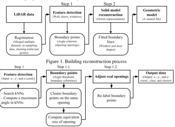
The proposed workflow can be divided (Figure 1): (i) initial feature detection, in which sample points (called boundary
points) lying on the façade and its openings are extracted by using the angle criterion and then unrealistic holes are eliminated by comparing characteristics of detected holes to standard building openings and (ii) geometric model reconstruction, in which a geometric model is produced.
Since the solid models herein are used for structural analy-sis, some non-structural elements (e.g. balconies and win-dow ledges) are not included. Further, this work assumes that buildings are quadrilateral in shape, with structural ele-ments residing within a planar façade, with openings com-prised of primarily rectangular windows and glass-plated doors, and currently only reconstructs two-dimensional (2D) façades but could be extended to 3D models.
3.1 Boundary detection (Step 1)
[image:4.595.120.480.405.666.2]As mentioned above, a pre-processing step classifies input sample points into boundary and interior classifications and discards unrealistic holes (Figure 2). There, each sample point is examined as to whether or not it lies on a boundary using an angle criterion. A boundary coherence technique (as will be discussed subsequently) is then applied to im-prove robustness. Holes are then assessed by comparing their characteristics to those of standard building openings. Their boundary points are finally re-classified as interior points, if they fail to meet the criteria (Figure 2).
Figure 1. Building reconstruction process
Figure 2. Feature detection processes
3.1.1 Angle criterion in boundary point detection (step 1.1)
Point, pi, is an “interior point” if the neighboring points are
distributed around an entity (Figure 3a), or a “boundary point”, if the neighboring points form a partial ball (Figure 3b). Thus, the maximum angle between two consecutive
boundary point, if the maximum angular gap exceeds an angular threshold. Otherwise, it is an interior point.
a) Neighbor points of an interior point, pi
b) Neighbor points of a boundary point, pi
Figure 3. Distribution of the number of nearest neighbor points of a given point
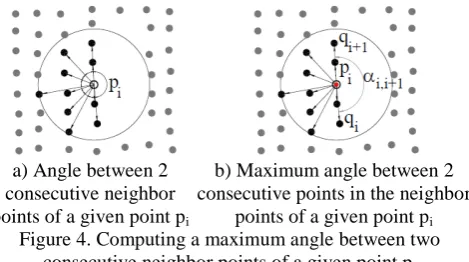
The FA algorithm starts with a randomly selected sample point and searches for a set of neighboring points, q (discussed below). The neighboring points, q, are projected onto a target-fitting plane (Figure 4). Cartesian coordinates of neighboring points are then transformed into relative cy-lindrical coordinates, with the local origin set at a given point pi. An angle between two consecutive neighboring
points, i,i+1 = qiqi+1, is computed as the difference
be-tween their azimuths (Figures 4a). The given point is label-ed as a boundary one, if the angle (i,i+1) exceeds a given
threshold (Figure 4b), and an interior point, otherwise.
a) Angle between 2 consecutive neighbor points of a given point pi
b) Maximum angle between 2 consecutive points in the neighbor
[image:5.595.55.272.93.211.2]points of a given point pi
Figure 4. Computing a maximum angle between two consecutive neighbor points of a given point pi
For selecting neighboring points of a given point, various methods have been used, such as a ball neighborhood (Fig-ure 5a) and kNN (Fig(Fig-ure 5b). Herein, a binary search k-di-mension (k-d) tree was implemented into the FA algorithm for searching kNN points, where each leaf node contains a number of predefined target points (Bentley, 1975) – e.g. the 20 points (as discussed subsequently) adopted in this k-d tree. A number of kNNs, q{q1, q2,…,qn}, the nearest
points of the given point, p, in the Euclidean distance, were extracted by the use of a k-d tree; [see Moore (1990) for more details of the searching].
Selecting am optimal number of kNN points is an important task, because this affects the running time and feature de-tection quality. For example, if the data have a high level of noise or are relatively sparse, selecting a small number of kNN points will lead to large errors in classification (e.g. a sample point in the sparse Figure 6a data set was classified as a boundary point instead of an interior one). Similarly, boundary points are overlooked with excessively large
neighborhoods (Figure 6b). Additionally, as point density varies within a data set, with low densities normally occur-ring in boundary areas, a neighborhood with a predefined number of kNN points can unintentionally contain sample points belonging to surface patches along two boundaries of the same opening (Figure 6b), which causes improper clas-sification. Herein it is proposed, that the problem can be minimized by implementing a radius threshold to constrain the ball of the neighborhood. In this, the ball’s radius must be less than or equal to the selected threshold. This thresh-old is set to a normal minimum window opening size (i.e. 0.4m) based on empirical work by (Pu & Vosselman 2007). The kNN searching algorithm implemented in this study is defined by an input number of kNN points combined with the neighborhood’s maximum radius (something not pre -viously done). Results with and without a radius threshold are illustrated in Figures 7a and 7b, respectively.
a) Ball searching algorithm with a pre-defined radius 0.5m
b) k-nearest neighbor searching for 10 kNNs Figure 5. Searching nearest neighbor point algorithm
a) 8 kNNs causing misclassification of point
pi in a sparse dataset
b) 22 kNNs causing misclassification of point pi due
[image:5.595.314.549.262.704.2]to overly large neighborhood Figure 6. Misclassification of sample points due to either an
overly sparse data or an excessively large neighborhood.
a) 15 kNNs with an upper bound searching radius leads
to only 13 kNNs selected
b) 15 kNNs without an upper bound searching
radius
Figure 7. Selecting 15 kNNs of the given point pi with and
without an upper bound searching radius
[image:5.595.48.283.381.512.2]the given point forming the maximum angle are also boun-dary points. Otherwise, the point is classified as an interior one. In this study, the process is used to check through all boundary points detected in the previous step.
3.1.2 Adjusting openings
To distinguish real from apparent openings, any detected hole is compared to a standard façade opening. A detected hole is presumed false, if its characteristics fail to meet pre-defined opening criteria (as will be discussed later). To make this check, firstly all points on the boundary of a single hole are clustered using a clustering technique with a predefined searching radius (Guha et al., 1999). The radius value must ensure that none of the boundary points of adja-cent openings are unintentionally included, while still cap-turing all the relevant boundary points (Figure 8a). In real buildings, the distance between adjacent rows or columns of openings or an opening and the façade edge is normally larger than 0.2m (Ripperda, 2008) [Figure 8b]. Thus, a pre-defined searching radius equal to 0.2m is adopted.
a) Clustering all boundary points of a selected opening
b) Unintentional selection boundary points from adjacent openings due to an overly large searching radius * Black points are respectively boundary points of windows
1 and 2
Figure 8. Clustering boundary points of the openings
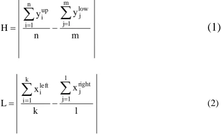
Next, characteristics of each detected hole (height, length, and height/length ratio) are computed using a histogram a-long the horizontal and vertical directions (Figure 9), where the hole is assumed to be rectangular. The possible hori-zontal and vertical boundary lines of a hole can be deter-mined from two peaks of the histogram along the x- and y-directions, respectively (Figure 9b and c), in which a num-ber of bins in each direction is adopted equal to 10. How-ever, for holes (such as doors) at the ground surface, only one peak on the upper side appears on the histogram along the y-direction. Based on this concept, equivalent dimen-sions (height and length) of each hole are consequently de-termined in accordance with equations 1 and 2.
m y
n y H
m
1 j
low j n
1 i
up
i
(1)
l x
k x L
l
1 j
right j k
1 i
left
i
(2)
where n and m, and k and l are a number of boundary points belonging to 2 peaks (“up” and “down”) along the y-histogram, and to 2 peaks (“left” and “right”) along the x -histogram. Notably, for a hole along the ground surface, the down peak is the lowest bin in the y-histogram.
a) Boundary points of the window
b) X-coordinate histogram of boundary points along the x-direction
[image:6.595.313.542.236.376.2]c) Y-coordinate histogram of boundary points along the y-direction Figure 9. Using histograms to determine height and length of a window
Finally, holes are categorized as occlusions, if their charac-teristics differ from a predefined minimum opening dimen-sions greater or equal to 0.4m (as established by Pu & Vosselman 2007) and a height (Ho) to length (Lo) ratio
greater than 0.25 and less than 5.0 (as established by Mayer & Reznik 2005; Ripperda 2008) (Equation 3). Thereafter,
openi ng Non : Ot her wi seOpeni ng : 0 . 5 L / H 25 . 0 ; m 4 . 0 L ; m 4 . 0 H i f L / H , L , H
f o o
o o o o o o (3)
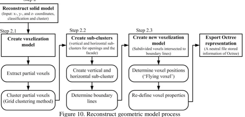
3. 2 Solid model reconstruction (Step 2)
The aim of Step 2 (Figure 10) is to reconstruct a solid mo-del of the building façade from raw data points adding a
[image:7.595.106.498.194.382.2]point classification of either “interior” or “boundary” as de-fined in Step 1. In surface reconstruction from a set of sample point, an object’s surface-based triangulation consists of curved surfaces, instead of the generally planar surface of building façades. Surface-based triangles may cause difficulty in generating FEM meshes or result in distorted FEM meshes leading to unstable numerical solution. For these reasons, voxelization is implemented into the FA algorithm to generate a complete building model.
Figure 10. Reconstruct geometric model process
Initially, a bounding box enclosing the building’s entire fa -çade is established. Often, a bounding box has equal edge lengths but is defined herein by equations (4) and (5) there-by implying the possibility of non-cubic voxels.
m i n m a x
BB x x
L (4)
m i m a x
BB y y
H (5)
where xmax, ymax, xmin, ymin are minimum and maximum
coordinates of input sample points.
In the proposed FA algorithm, a voxel’s size along its short side (either longitudinal or vertical) of the façade is less than half of the minimum feature size (e.g. if the minimum opening dimension is 0.4m, voxel size must be less than 0.2m.). Thus, the required octree depth along x- an y-directions can be given:
ze Mi nVoxel Si
L l og
x _
dept h 2 BB (6)
ze Mi nVoxel Si
H l og
y _
dept h 2 BB (7)
in which MinVoxelSize = 0.2 m and the sign [] means that the value is rounded up toward the nearest integer. As the octree depth is unique, the maximum octree depth for recursively subdividing in this proposed approach can expressed as:
max_Octree_depth = max(depth_x, depth_y) (8)
Subsequently, an initial voxel is subdivided along the x- and y-directions into four smaller voxels. Herein, the voxel
is then categorized as “Empty”, “Full” or ”Partial”. The voxel is “Empty”, if it contains no data points, or “Full” if it
contains exclusively interior points. The last category is
“Partial”, if the voxel contains interior and boundary points or only boundary points. In the three sample buildings to be presented in the experimental section a depth of 8 was found to be ideal for the smaller structures and a depth of 9 for the larger.
Boundary lines of the building façade and its openings are determined based on boundary points underlying partial voxels. To achieve this, a group of empty voxels is assumed to be inside an opening, and then the partial voxels around the opening are clustered using a flood-filling algorithm (Agoston, 2005), in which 8 voxels connected to the se-lected voxel are checked.
im-plementing a constrained condition in the grid clustering technique, incorrect boundary points due to noise in the data can be eliminated, because those boundary points may be stored as partial voxels on fragment girds. Often, the boundary points for reconstructing boundary lines lie in the same grid voxels, which implies a low noise level for these points.
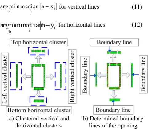
Furthermore, these grid clusters are classified as sub-cluster voxels containing boundary points representing boundary
lines for each opening’s side by comparing coordinates of
the grid cluster voxels to coordinates of the opening’s centre (Figure 11a). For example, a window has four sub-cluster voxels corresponding to the four boundary lines (two vertical, one bottom, and one top), whereas a ground-floor door normally includes only three representing to three boundary lines (no bottom boundary lines). For gene-rating two vertical lines and a bottom boundary line, these line segments were determined based on coordinates of all boundary points contained within the sub-cluster’s voxels by using a least median of squares approach (Pighin & Lewis, 2007, Fleishman et al., 2005). To obtain realistic vertical and horizontal boundary lines, fitting lines were de-termined from a set of boundary points in each sub-cluster S = {pi = (xi,yi, zi)| 1≤ i≤n} as shown in equation 9 and 10.
x = a for vertical lines (9)
y = b for horizontal line (10)
where the parameters a and b were determined by minimizing the median of the residuals:
i i
a
x a m edi an m i n
ar g for vertical lines (11)
i i
b
y
b
med ian
min
arg
for horizontal lines (12)a) Clustered vertical and horizontal clusters
[image:8.595.44.285.438.647.2]b) Determined boundary lines of the opening
Figure 11. A modified grid clustering technique is employed to cluster vertical and horizontal voxels and to
determine boundary lines of the opening
For the detailed process for parameter determination see Pighin & Lewis (2007) and Fleishman et al. (2005). This technique can eliminate 50% of all outlier points (Fleishman et al., 2005). Additionally, as the top boundary lines of real openings may be straight (as in rectangular openings,) bi-linear (as in wedge openings) or curved (as in arched openings), the y-coordinates of the end points of the top line were determined from average y-coordinates of these boundary points, while x-coordinates of the end points were set equal to two outlier boundary points along horizontal direction. A similar process was applied for
determining the façade’s boundary lines.
The full voxels were then stored in a database to describe the geometric model of the solid wall for computational modeling. Thus, the properties of the voxels must be re-classified based on their positions. Namely, the empty
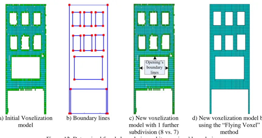
voxels are either “inside” openings (interior to a set of an opening’s boundary lines) or outside the façade (exterior to a set of the façade’s boundary lines). To achieve this, a fur -ther voxelization is created by dividing the initial voxeli-zation model (Figure 12a) by the boundary lines (Figure 12b). For this, the number of child voxels depends on the number of boundary lines intersecting a parent voxel. For example, four child voxels would be created, if two boun-dary lines intersected the parent voxel. Conversely, no sub-division would occur, if no boundary line intersected the parent voxel, or if boundary lines(s) coincided with surface plane(s) of the parent voxel.
In re-voxelization (Figure 12c), voxels inside of openings or outside of the façade are now labeled as empty and all others as full. For that, the “Flying Voxel” method (Truong -Hong et al., 2012) is employed to quickly determine one of three possible positions with respect to various boundary lines: Case 1 - voxel outside of the façade; Case 2 - voxel inside the façade and inside an opening; or Case 3 - voxel in-side the façade but not inside any opening. This approach is summarized in Truong-Hong et al. (2012).
a) Initial Voxelization model
b) Boundary lines c) New voxelization model with 1 further subdivision (8 vs. 7)
d) New voxelization model by
using the “Flying Voxel”
[image:9.595.80.511.65.292.2]method Figure 12. Determined façade boundaries and its openings’ boundaries
4 EXPERIMENTAL RESULTS AND DISCUSSION
To validate the algorithms, four datasets were created for each of three brick buildings in Dublin, Ireland (Figures 13a-15a), which were selected for their proximity to an up-coming metro project and the availability of independent survey measurements. TLS point cloud data were collected using a Trimble GS200 device. Point clouds of each build-ing acquired from multiple scanner stations because of traf-fic, terrain limitations, and footpath space were registered by using RealWork Survey (RWS) V6.3, proprietary soft-ware associated with the Trimble GS200 scanner. In this survey, two scanner stations were set up for each building. A minimum of three reference regions for each scanner sta-tion was acquired at 2 mm resolusta-tions in order to merge pointclouds of the façade, in which the reference regions were chosen at well-defined positions such as window cor-ners or window ledges. A trial and error merge process was manually undertaken by selecting a pair of points from the source and target stations until the average error of each tar-get point expressed in term of distance errors was less than 5mm. Additionally, sampling point clouds were obtained by using a random sampling function built on RWS, in which a required distance between two adjacent sample points was defined.
The first set was the original scans (NS00) after being co-registered and having points +/-20 cm behind the expected building façade removed. The other three were subsets using random re-samplings with expected distances between sampling points of 20mm (S20-2500pts/m2), 50mm (S50-400pts/m2) and 75mm (S75-175pts/m2) [Table 1]. The densities were selected to test algorithm sensitivity.
For extracting only sample points of considered facades, a MATLAB subroutine incorporated with MATLAB libraries
was developed. Point clouds of adjoining building were re-moved. Similar to work of Adan and Huber (2011), the fa-çade surface was determined from a histogram peak along depth direction. For that, points ±20 cm from the facade were considered as sample points of objects behind the fa-çade (e.g. floors, internal walls and objects) or non-func-tional structures in front of the façades and were manually removed. Finally, the ground level was also determined as a peak of a histogram along vertical direction.
Table 1. Dataset Sizes
Building Sampling dataset NS00 S20 S50 S75
B1: 2 Anne St. South 264,931 51,171 9,909 4,643
B2: 5 Anne St. South 190,865 51,884 11,119 5,366
B3: 2 Westmoreland St. 650,306 353,848 71,155 35,468
[image:9.595.316.550.421.512.2]a) Photo Building 1 (4.95m w x12.16m h)
b) Scanning data in the RealWorks Survey program
c) Point cloud after cleaning and resampling
d) Boundary points in red
e) Initial voxel representation
f) Voxel representation subdivided by boundary lines
g) Solid model representation
h) CAD drawing from physical survey(*)
[image:10.595.68.529.72.365.2](*) values in [] are derived from the FA algorithms, while others are the independently measured survey values
Figure 13. Facade reconstruction for Building 1 based on dataset of 2500pts/m2 (S20-distance between adjacent sample points no less than 20mm)
a) Photo Building 2 (4.90m l x 13.28m h)
b) Scanning data in the RealWorks Survey program
c) Point cloud after cleaning and resampling
d) Boundary points in red
e) Initial voxel representation
f) Voxel representation subdivided by boundary lines
g) Solid model representation
h) CAD drawing from physical survey(*)
(*) values in [] are derived from the FA algorithms, while others are the independently measured survey values.
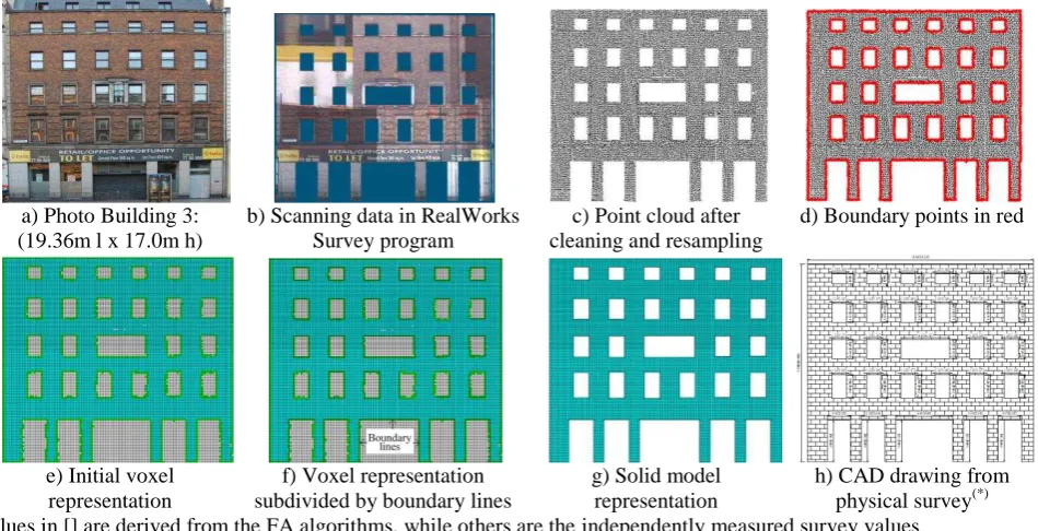
[image:10.595.80.532.393.726.2]a) Photo Building 3: (19.36m l x 17.0m h)
b) Scanning data in RealWorks Survey program
c) Point cloud after cleaning and resampling
d) Boundary points in red
e) Initial voxel representation
f) Voxel representation subdivided by boundary lines
g) Solid model representation
h) CAD drawing from physical survey(*)
(*)
[image:11.595.62.537.74.317.2]values in [] are derived from the FA algorithms, while others are the independently measured survey values Figure 15. Facade reconstruction for Building 3 based on a dataset of 175 pts/m2
(S75-distance between adjacent sample points no less than 75mm)
5 GEOMETRIC VALIDATION
Geometric accuracy of building façades in figures 13a, 14a, and 15a derived from the FA approach was compared to those processed in the commercial program, Kubit (1999). In this comparison, the building facades from on-site survey
are considered for benchmarking quantities. In Kubit, the solid models were created within an AutoCAD program by manually indentifying openings and building boundaries
based on a building’s photograph. Building façades
generated from the Kubit program based on input datasets in Figure 13c, 14c and 15c are shown in Figure 16.
a) Building 1 b) Building 2 c) Building 3
Figure 16. Building façades created by Kubit program based on input datasets in Figure 13c, 14c and 15c
To evaluate accuracy, the geometries of the derived building models were compared to measured drawings from independently produced on-site surveys (Figure 13h, 14h and 15h). In general, length of building models derived from the FA algorithm were slightly underestimated while
[image:11.595.72.528.420.697.2]Kubit program overestimated Building 1 by 3% (Figue 17a). Similarly, the FA algorithm also tended to underestimate the building height, whereas the Kubit program tended to overestimate it. While, the relative errors of the building height from the FA algorithm were slightly
higher than ones from the Kubit program, the maximum relative errors were no more than 1.2% (Building 3) for the FA-based models versus 0.6% for the Kubit-based models (Figure 17b), with the benefit of the FA algorithm being fully automated.
[image:12.595.81.515.135.240.2]a) Lengths b) Heights c) Opening area
Figure 17. Relative errors of building facades reconstructed by FA algorithm and Kubit program compared to independently measured drawings
In terms of opening areas, for the small buildings (Building 1 and 2), the FA algorithm was more accurate (maximum relative error of 3.7% for Building 2) than the Kubit program generated ones (maximum relative error of -7.2% for Building 2), as shown in Figure 17c. However, for the larger Building 3, the opposite trend was found with the FA algorithm overestimating the opening area by 3% and the Kubit program underestimating by 1% (Figure 17c). As the resulting geometry of the building components (e.g. openings) may or may not affect building response depending upon the application, the geometric accuracy of the components was also evaluated.
By considering the most important building components in masonry buildings (e.g. openings), the approach was also shown to be comparable. The average absolute errors of the opening dimensions in the FA-based solid models were generally less than the Kubit-based ones (Table 2), in which the average error was 12.7mm [Standard deviation (SD)=121.1mm] in Building 2or the FA-based models, while 75.6mm (SD=102.7mm) for the Kubit-based ones. However, for the larger Building 3, opening dimensions in the Kubit-based model were more accurate than those from the FAbased models. For that, the average errors were -30.3mm (SD=54.1mm) and 4.5mm (SD=58.6mm) for the FA- and Kubit-based models. In conclusion, the FA algorithm more commonly automatically generated building models of superior accuracy than those created by the operator-assisted Kubit ones. This was likely caused by the fact that the Kubit program depends on visual interpolation by the user, while the FA algorithm generates the boundaries of the façade and its openings strictly from
[image:12.595.316.550.321.399.2]sample points.
Table 2. Geometric differences between CAD drawings against the FA and Kubit-based solid models
Aspects (mm)
Building 1 Building 2 Building 3 FA-S20 Kubit FA-S50 Kubit FA-S75 Kubit Average 8.6 28.8 12.7 75.6 -30.3 4.5 Min. error -109.0 -110.0 -165.0 -40.0 -177.0 -140.0 Max. error 179.0 250.0 359.0 370.0 45.0 70.0 Stand. dev. 111.4 110.0 121.1 102.7 54.1 58.6
5.1 Quality of boundary point detection
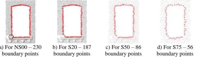
The proposed FA algorithm consistently detected all openings for each of the three building facades (Figure 13-15). Using 20 kNNs, sufficient boundary points were found on the façade boundaries and its openings to reconstruct realistic boundary lines (Figure 13c, 14c and 15c), with improved detection for denser datasets (Figures 18a-b vs. Figures 18c-d). Notably, the FA algorithm can detect all boundary points around openings corners, a shortcoming that occurs in the Delaunay triangulation based FD algorithm (Truong-Hong et. al, 2011) [Figure 19] or with use of a shape criterion (Becker & Haala, 2007). Additionally, the FA algorithm also detected approximately
twice the number of boundary points on building’s features
than the FD algorithm (Figure 18 vs. Figure 19), even in the presence of occlusions (Figure 18a black circle). This opens the way for further processing options or further density reductions, which may soon enable use of existing ALS data for solid model generation of building facades.
a) For NS00 – 230 boundary points
b) For S20 – 187 boundary points
c) For S50 – 86 boundary points
[image:12.595.126.474.647.748.2]d) For S75 – 56 boundary points
a) For NS00 – 71 boundary points
b) For S20 – 61 boundary points
c) For S50 – 42 boundary points
[image:13.595.331.532.324.439.2]d) For S75 – 32 boundary points
Figure 19. Boundary points of a top left window of Building 2 with various sampling density of datasets from the FD algorithm (adapted from Truong-Hong et al. 2012)
5.2 Processing time
The majority of the total processing time was devoted to feature detection (Figure 20). With a dataset of 190,865 points [as shown as 5.28 (log190,865) on x-axis of Figure 20], the feature detection took 102.3 minutes while voxelization required only 1.8 minutes (Figure 20). This is because the feature detection algorithm must pass through the entire dataset, whereas the voxelization process is mainly searching through partial voxels to reconstruct
boundary lines of building’s features. The voxelization process depends on not only depth of octree representation but also the number of openings needing to be reconstructed. For example, the process took 0.8 minutes for Building 2 (51,884 sample points, 8 openings and depth of octree representation by 8) but 6.28 minutes for Building 3 (71,155 sample points, 28 openings and depth of octree representation by 9; the greater size of Building 3 required an additional level of division).
While, the FA and FD algorithms (Truong-Hong et al., 2012) were nearly equivalent in speed, particularly for datasets less than 350k sample points, the FA algorithm may be further optimized, by having the feature detection portion of the algorithm search only on the sample points around openings instead through all sample points, as currently reflects its implementation.
a) Feature detection
b) Voxelization process
Figure 20. Running time of the algorithms.
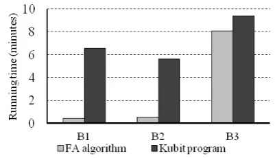
To investigate efficiency of the proposed FA algorithm and Kubit program in reconstructing building models, the dataset of S75 was selected and the results of the building models was illustrated in Figure 13-16. Processing time for manual cleaning irrelevant points with the RealWork Survey is 5 minutes for all datasets while ones for reconstructing the building models is shown in Figure 21 (below). In general, the FA algorithm is faster than the Kubit program, particularly for small buildings (Building 1 and 2) having less number of openings.
Figure 21. Comparing processing time between FA algorithm and Kubit program based on dataset of S75
5.3 Influence of critical input parameters
In the angle criterion, the vital parameters were identifying the critical angle and selecting a suitable neighborhood. In this study, the critical angle was set equal to /2, which worked well, even in the corners, because the data points were fairly regularly distributed. False results occur, if the number of kNNs is set either too low or too high. As such, as discussed previously, for cases of 8 or 22 kNNs selected, detection of either interior or boundary points would be incomplete (Figure 6). By assuming a perfectly distributed rectangular data set, 8 kNN points would be sufficient for boundary point detection (Figure 22 with sample points in circles), but real data are not distributed as such. Thus, 20 kNN points were selected for all datasets, corresponding to
0.2m of the ball’s radius of the kNN points for 75mm
sampling dataset. This selection provides rapid boundary point detection while avoiding accidental sample point collection on adjacent openings. Additionally, the 0.2m radius enabled robust clustering of all boundary points on
the boundaries of the façade’s features for each of the 12
[image:13.595.85.239.518.741.2]Note:
* Dark gray points: sample points * Black gray points: given points * Unfilled circle points: boundary points * Black points: neighbor points
* Circles: selecting 8 kNN points
[image:14.595.69.533.445.686.2]* Dash lines: an expected window boundary lines Figure 22. Selecting neighboring points in rectangular
distribution of sample points
6 NUMERICAL ASSESSMENT
As the main goal of the FA algorithm was to reconstruct solid models of existing building façades for computational modeling, compatibility of the solid models and the impact of the aforementioned geometric discrepancies on numerical results must be discussed. To evaluate the usability of these models for a relevant case, the responses of the FEM models derived solid models from the FA algorithm were compared to ones based on CAD drawings from on-site drawings submitted for planning permission. In this section, the solid models of Building 1 respectively shown in Figure 13g and 13h for the FA algorithm and the
CAD drawing were selected for further investigation.
Non-linear analysis was adopted for analyzing the solid model of Building 1 by using ANSYS Mechanical APDL product (ANSYS Academic Research Release 13.0), where a macro modeling strategy was employed to model the building facade by using a SOLID65 element. Additionally, a William Warnke (WW) failure criterion and Drucker-Prager (DP) yield criterion built into the ANSYS program are respectively to model masonry behavior in tension and compression. Thus, the WW failure criterion provides a tension cut-off for the DP yield criterion (Truong-Hong and Laefer, 2008). Material properties were selected from existing experimental reports and the peer-reviewed literature to represent medium-strength masonry properties used for this analysis. These were as follows: for elastic
behavior Young’s modulus of 3,480 MPa and Poisson’s
ratio 0.16 and for plastic behavior for 26.15/1.15 MPa of compressive/tensile strength, 6.81 MPa internal cohesion, 350 internal friction angle and 100 dilatancy angle. The analysis was conducted under self-weight and imposed displacements due to excavation-induced foundation settlements (Truong-Hong 2011), in which an element size of 0.15 m was predefined for FEM mesh generation, and displacements were directly applied to nodes on the bottom of the model (Figure 23a and b). As discrepancy of building length (Figure 17a) and the building edge is set at 2 m behind excavation face (Truong-Hong, 2011), there are small different displacements imposed on FEM models based on CAD drawing and the FA algorithm, where the minimum displacements were respectively 24.764 mm and 24.905 mm (Figure 23a and b).
a) FEM mesh & imposed displacement – CAD based
b) FEM mesh & imposed displacement – FA based
c) Displacements of FEM model – CAD based
d) Displacements of FEM model – FA based
Figure 23. Finite element models and numerical results from CAD and FA based models
Graphically, the numerical analysis showed a consistency of nodal displacements between the FEM models based on two sources of the solid models (Figure 23c and d). The maximum nodal displacement differed by no more 1.6%, with an absolute difference of only 1.6 mm (Figure 23). In terms of an engineering perspective, this difference in FEM
computational models from TLS data.
7 CONCLUSIONS AND FUTURE WORK
The newly proposed FacadeAngle algorithm combines an angle criterion, voxelization, and the positional determining Flying Voxel method to automatically extract building façades and their major features from LiDAR point cloud data for further computational modeling. By use of an angle threshold combined with a pre-specified searching radius and a pre-selected number of nearest neighbor candidates, the algorithm performed within acceptable limits in a wide variety of tests against a semi-automatic, commercial alternative on three urban buildings at 4 data densities. Favorable results were also obtained for geometric variance of the overall form and individual elements compared to solid models derived from measured drawings, as well as for resulting displacements and stresses in an adjacent excavation scenario (within 1.6% or 1.6 mm). Furthermore, even without full optimization, the processing time was comparable to another voxel-based automated approach and was also able to automatically overcome holes caused by data occlusions. In addition to these favorable aspects, the strategic advantages that the FacadeAngle potentially possesses over other approaches are as follows:
1. Ability to precisely detect all boundary points around the corners of openings, except where occlusions exist
2. Capability to harvest twice the number of boundary points over other automated methods
3. Item 2 offers the potential for further processing for more exact results and/or for the abandonment of any a priori knowledge (e.g. general window sizes); something not yet obtainable in any approach
4. Item 2 also offer the potential use of less dense data sets, such as aerial ones in the near term as there is a difference of two orders of magnitude between current high level aerial data when vertically projected and the typical terrestrial scan.
However, the proposed algorithm needs to be extended to non-rectangular forms, optimized for use with large and sparse datasets, and needs to be freed from reliance on prior knowledge. Finally, increasing automation and applicability of this method will require its extension to fully 3D models and its integration with a procedure appropriate to eliminate irrelevant sample points prior to the initial processing.
ACKNOWLEDGMENTS
This work was made possible through the generous funding of Science Foundation Ireland (SFI/PICA/I850). Thanks to Donal Lennon of Urban Institute Ireland for assistance with data acquisition.
REFERENCES
Adan, A., Huber, D., (2011), 3D reconstruction of interior wall surfaces under occlusion and clutter, 3D Imaging, Modeling, Processing, Visualization and Transmission (3DIMPVT) May 16-19, 2011, 275-81.
Agoston, M. K. (2005), Computer Graphics and Geometric Modeling: Implementation and Algorithms, Springer Verlag London Ltd.
Ali, H., Ahmed, B., & Paar, G. (2008), Robust window detection from 3d laser scanner data, 2008 Congress of Image and Signal Processing, Hainan, China, May 27-30, 2008, 115-118.
Alshawa, M., Boulaassal, H., Landes, T., & Grussenmeyer, P. (2009), Acquisition and automatic extraction of facade elements on large sites from a low cost laser mobile mapping system, 3D-ARCH 2009, 3D Virtual Reconstruction and Visualization of Complex Architectures, Feb. 25-28, 2009, Trento, Italy, 6p.
ANSYS Academic Research Release 13.0, Help System, Theory Reference for ANSYS and ANSYS Workbench.
Becker, S. & Haala, N. (2007), Refinement of building fa-cades by integrated processing of LiDAR and image data, PIA07 - Photogrammetric Image Analysis, Munich, Germany, Sept. 19-21, 2007, 7-12.
Becker, S. & Haala, N. (2009), Grammar supported facade reconstruction from mobile LiDAR mapping, CMRT09-City Models, Roads and Traffic, Paris, France, Sept. 3-4, 2009, 229-234.
Bendels, G. H., Schnabel, R., & Klein, R. (2006), Detecting Holes in point set surfaces, Journal of WSCG, 14.
Bentley, J. L. (1975), Multidimensional binary search trees used for associative searching, Communications of the ACM, 18(9), 509-517.
Berg, M. D., Krefeld, M. v., Overmars, M., & Schwarzkopf, O. (2000), Computational Geometry: Algo-rithms and Applications, Springer.
Böhm, J., Haala, N., & Becker, S. (2007), Façade model-ling for historical architecture. XXI International CIPA Symposium, 1-6 Oct., Athens, Greece. 2007, 7pp.
Boulaassal, H., Chevrier, C., & Landes, T. (2010), From laser data to parametric models: towards an automatic method for building façade modelling, Digital Heritage: Third International Euro-Mediterranean Conference, Lemessos, Cyprus, Nov. 8-13, 2010, 42-55.
Boulaassal, H., Landes, T., & Grussenmeyer, P. (2009), Automatic extraction of planar clusters and their contours on building façades recorded by terrestrial laser scanner, International Journal of Architectural Computing, 7(1) 1-20.
Cai, H., & Rasdorf, W. (2008), Modeling road centrelines and predicting lengths in 3d using LiDAR point cloud and planimetric road centreline data, Computer-Aided Civil and Infrastructure Engineering, 23(3) 157-173.
Dorninger, P., & Pfeifer, N. (2008), A comprehensive automated 3d approach for building extraction, recon-struction, and regularization from airborne laser scanning point clouds, Sensors, 8(11) 7323-7343.
reconstruction, International Archives of the Photogrammetry, Remote Sensing and Spatial Information Sciences, 38 (Part 3/W8), 49-54.
Guha, S., Rastogi, R., & Shim, K. (1999), ROCK: A robust clustering algorithm for categorical attributes, Fifteenth International Conference Data Engineering, Sydney, Australia, Mar. 23-26, 1999, 512-21.
Gumhold, S., Wang, X., & Macleod, R. (2001), Feature extraction from point clouds, Proceedings 10th International Meshing Roundtable, Sandia National Laboratory, Oct. 7-10, 2001, 293-305.
Hinks, T. (2011), Geometric processing techniques for urban aerial laser scan data, PhD thesis, University College Dublin, Dublin, Ireland.
Hinks, T., Carr, H., Laefer, D.F., O’Sullivan, C., Morvan,
Y., Truong-Hong, L., & Ceribasi, S. (2008), Robust building outline extraction. PTO 56793223.
Hinks, T., Carr, H., & Laefer, D. (2009), Flight optimization algorithms for aerial LiDAR capture for urban infra-structure model generation, Journal of Computing in Civil Engineering, 23(6) 330-339.
Hoffman, E.S., Gustafson, D.P., Gouwens, A.J., Rice, P.F. (1996), Structural Design Guide to the AISC (LRFD) Specification for Buildings, 2nd ed., Chapman and Hall, London.
Hohmann, B., Krispel, U., Havemann, S., & Fellner, D. (2009), CITYFIT: High quality urban reconstructions by fitting shape grammars to images and derived textured point clouds, ISPRS, Remote Sensing and Spatial Information Sciences, 38(Part 5/W1), CD-ROM.
Hoppe, H., Duchamp, T., McDonald, J., Stuetzle, W. 1992, Surface reconstruction from unorganized points, Proceeding of SIGGRAPH '92, Chicago, IL, Jul. 27-31, 1992, 71-78.
Huber, D., Akinci, B., Oliver, A.A., Anil, E., Okorn, B.E. & Xiong, X. (2011), Methods for automatically modeling and representing as-built building information models, Proc. NSF CMMI Research Innovation Conf., http://www.-ri.cmu.edu/pub_files/2011/1/2011-huber-cmmi-nsf-v4.pdf
Laefer, D.F., Hinks, T., & Carr, H. (2010), New possibilities for damage prediction from tunnel subsidence using aerial LiDAR data, ISSMGE, Geotechnical Challenges in Megacities, Moscow, Russia, Jun. 7-10, 2010, 622-629.
Laefer, D.F., & Pradhan, A. (2006), Evacuation route selection based on tree-based hazards using LiDAR and GIS, Journal of Transportation Engineering, 132(4) 312-320.
Laefer, D.F., Truong-Hong, L., & Fitzgerald, M. (2011a), Processing of terrestrial laser scanning point cloud data for computational modelling of building facades, Recent Patents on Computer Science, 4(3) 16-29.
Laefer, D.F., Hinks, T., Carr, H., & Truong-Hong, L. (2011b), New advances in automated urban model
population through aerial laser scanning. Engineering Patent Journal, 5(3) 196-208.
Lee, H. M., & Park, H. S. (2011), Gage-Free stress estimation of a beam-like structure based on terrestrial laser scanning, Computer-Aided Civil and Infrastructure Engineering, 26(8) 647-658.
Linsen, L., & Prautzsch, H. (2001), Local versus global triangulations, EUROGRAPHICS 2001, Manchester, England.
Linsen, L., & Prautzsch, H. (2002), Fan clouds - an alter-native to meshes, 11th International Workshop on Theoretical Foundations of Computer Vision, Dagstuhl Castle, Germany, Apr. 7-12, 2002, 451-471.
MathWorks. (2007), MATLAB Function Reference.
Mayer, H., & Reznik, S. (2005), Building façade interpretation from image sequences, CMRT 2005-Object Extraction for 3D City Models, Road Databases and Traffic Monitoring - Concepts, Algorithms and Evaluation, Vienna, Austria, Aug. 29-30, 2005, 55-60.
Moenning, C., & Dodgson, N. A. (2004), Intrinsic point cloud simplification, Graphicon'04 - International. Conference on Computer Graphics and Vision, Moscow, Russia, Sept. 6-10, 2004.
Moore, A.W. (1990), Efficient memory-based learning for robot control, PhD thesis, University Cambridge, Cambridge, UK.
Park, H. S., Lee, H.M., Adeli, H., Lee, I. (2007), A new approach for health monitoring of structures: terrestrial laser scanning, Computer-Aided Civil and Infrastructure Engineering, 22(1) 19-30.
Pighin, F. & Lewis, J.P. (2007), Practical least-squares for computer graphics, ACM SIGGRAPH 2007 courses, 1-57.
Pu, S. & Vosselman, G. (2007), Extracting windows from terrestrial laser scanning, ISPRS Workshop Laser Scanning and SilviLaser 2007, Espoo, Finland, Sept. 12-14, 2007, 320-25.
Pu, S. & Vosselman, G. (2009), Knowledge based reconstruction of building models from terrestrial laser scanning data, ISPRS Journal of Photogrammetry and Remote Sensing, 64(6) 575-584.
Ripperda, N. (2008), Determination of facade attributes for facade reconstruction, ISPRS, Beijing, China, Jul 3-11, 2008, 285-290.
Samet, H. (2008), K-Nearest neighbor finding using MaxNearestDist, Pattern Analysis and Machine Intelligence, 30(2) 243-252.
Truong-Hong, L. (2011), Automatic generation of solid models of building facades from LiDAR for computational modelling, PhD thesis, University College Dublin, Dublin, Ireland.
Computational Solid Mechanics, Nov. 27-30, 2008, Ho Chi Minh City, Vietnam, 241-250.
Truong-Hong, L., Laefer, D.F., Hinks, T., & Carr, H., (2012), Flying voxel method with Delaunay triangulation criterion for façade/feature detection for computation, Journal of Computing in Civil Engineering, http://dx.doi.org/10.1061/(ASCE)CP.1943-5487.0000188.
Tsai, Y., Wu, J., Wang, Z., & Hu, Z. (2009), Horizontal roadway curvature computation algorithm using vision technology, Computer-Aided Civil and Infrastructure Engineering, 25(2) 78-88.
Tang, P., Huber, D., & Akinci, B. (2009), Characterization of laser scanners and algorithms for detecting flatness defects on concrete surfaces, Journal of Computing in Civil Engineering, 25(1) 31-42.
Várady, T., Facello, M.A., & Terék, Z. (2007), Automatic extraction of surface structures in digital shape reconstruction, Computer Aided Design, 39(5) 379-388.
Wang, R., Bach, J., & Ferrie, F.P. (2011), Window detection from mobile LiDAR data, IEEE Workshop Applied Computer Vision, Kona, Hawaii, Jan. 5-7, 2011, 58-65.
Wang, K.C.P., Hou, Z., & Gong, W. (2010), Automated road sign inventory system based on stereo vision and tracking, Computer-Aided Civil and Infrastructure Engineering, 25(6) 468-477.
Wenisch, P., Treeck, C.V., Borrmann, A., Rank, E., & Wenisch, O. (2007), Computational steering on distributed systems: indoor comfort simulations as a case study of interactive CFD on supercomputers, International Journal of Parallel, Emergent and Distributed Systems, 22(4) 275-291.
Weyrich, T., Pauly, M., Heinzle, S., Scandella, S., & Gross, M. (2004), Post-processing of scanned 3d surface data, Symposium on Point-Based Graphics, ETH Zurich, Switzerland. Jun. 2-4, 2004, 85-94.
Wonka, P., Wimmer, M., Sillion, F., & Ribarsky, W. (2003), Instant architecture, ACM SIGGRAPH 2003, San Diego, California, Jul. 27-31, 2003, 669-677.
Zalama, E., Gómez-García-Bermejo, J., Llamas, J., & Medina, R. (2010), An effective texture mapping approach for 3d models obtained from laser scanner data to building documentation, Computer-Aided Civil and Infrastructure Engineering, 26(5) 381-392.
Zhang, C., & Elaksher, A. (2011), An unmanned aerial vehicle-based imaging system for 3d measurement of unpaved road surface distresses, Computer-Aided Civil and Infrastructure Engineering, 27(2) 118-129.
![Figure 13. Facade reconstruction for Building 1 based on dataset of 2500pts/m values in [] are derived from the FA algorithms, while others are the independently measured survey values 2 (S20-distance between adjacent sample points no less than 20mm)](https://thumb-us.123doks.com/thumbv2/123dok_us/7985473.203847/10.595.80.532.393.726/facade-reconstruction-building-algorithms-independently-measured-distance-adjacent.webp)