This is a repository copy of Do not only connect: a model of infiltration-excess overland flow based on simulation.
White Rose Research Online URL for this paper: http://eprints.whiterose.ac.uk/101765/
Version: Accepted Version
Article:
Kirkby, MJ (2014) Do not only connect: a model of infiltration-excess overland flow based on simulation. Earth Surface Processes and Landforms, 39 (7). pp. 952-963. ISSN
0197-9337
https://doi.org/10.1002/esp.3556
© 2014 John Wiley & Sons, Ltd. This is the peer reviewed version of the following article: Kirkby, MJ (2014), Do not only connect: a model of infiltration-excess overland flow based on simulation. Earth Surf. Process. Landforms, 39(7): 952–963, which has been published in final form at http://dx.doi.org/10.1002/esp.3556. This article may be used for
non-commercial purposes in accordance with Wiley Terms and Conditions for Self-Archiving. Uploaded in accordance with the publisher's self-archiving policy.
Reuse
Items deposited in White Rose Research Online are protected by copyright, with all rights reserved unless indicated otherwise. They may be downloaded and/or printed for private study, or other acts as permitted by national copyright laws. The publisher or other rights holders may allow further reproduction and re-use of the full text version. This is indicated by the licence information on the White Rose Research Online record for the item.
Takedown
If you consider content in White Rose Research Online to be in breach of UK law, please notify us by
Do not only connect: A model of infiltration-excess overland flow based on simulation.
Mike Kirkby, School of Geography, U. Leeds, UK
Abstract
The paper focusses on connectivity in the context of infiltration-excess overland flow and its integrated response as slope-base overland flow hydrographs. Overland flow is simulated on a sloping surface with some minor topographic expression and spatially differing infiltration rates. In each cell of a 128 x 128 grid, water from upslope is combined with incident rainfall to generate local overland flow, which is stochastically routed downslope, partitioning the flow between downslope neighbours.
Simulations show the evolution of connectivity during simple storms. As a first
approximation, total storm runoff is similar everywhere, discharge increasing proportionally with drainage area. Moderate differences in plan topography appear to have only a second order impact on hydrograph form and runoff amount.
The model has also been applied to a 10-year rainfall record, using both hourly and daily time steps, and the implications explored for coarser scale models. Initial trails incorporating erosion, continuously update topography and suggest that successive storms produce an initial increase in erosion as rilling develops, while runoff totals are only slightly modified. Other factors not yet considered include the dynamics of soil crusting and vegetation growth.
Introduction
Over the last ten years, the number of articles and citations for the term ‘connectivity’, in the contexts of both hydrology and geomorphology has increased greatly, with over thirty new articles year now published in ISI journals and over 800 citations a year in 2010-2012 (Web of Science, 2012). The concept of connectivity has been even more widespread in the ecological literature, particularly with the introduction of circuit theory, using the concept of conductance defined for all habitat and matrix areas to define potential for migration between areas for a species.
Initial concepts of connectivity have focused on the presence or absence of point-to-point connections between pairs of points (Bracken & Croke, 2007) or between regions (Bartel et al, 2011). In ecological contexts where there is no directional structure, connection between points can be powerfully extended through conductance models (McRae, 2008) but these have little applicability in hydrology, where flow is strongly directed downslope.
steady state for a conservative system. Detailed descriptions of dynamic connectivity between adjacent points across an area form one critical ingredient of fine scale process-based
models, such as CRUM (Reaney et al, 2007) or MAHLERAN (Wainwright et al, 2008). In this way, connectivity provides a valuable way of conceptualizing the local persistence and continuity of overland flow, particularly in semi-arid areas with short bursts of rainfall and patchy surface properties (e.g. Cammeraat, 2002). For time-spans over which the soils and topography can respond, the division between structural and functional connectivity
(Wainwright et al, 2011) is also valuable; structure providing a necessary pre-condition for functional connection, and function a conditioning set of drivers for change in structure.
To generalise response beyond the strictly local scale, it has seemed valuable to collapse the detail of overland flow connectivity into summary index variables, providing one or a few parameters that, for example, scale the response of a hillslope or small catchment to storm rainfall (e.g. Stieglitz et al, 2003, Bracken and Croke, 2007, Lane et al, 2009). Candidate indices include average travel times from runoff generating cells, average residence times and contributing areas, all potentially time-varying in response to catchment condition and storm rainfall. Although no magic bullet has yet emerged (e.g. Bracken et al, 2013) to summarize the complexity of hillslope or catchment response, it is helpful to observe, through
simulations, how and why topography and soil properties influence the runoff generated from an area.
The discussion here is also focussed on the response of semi-arid areas, where runoff generation is assumed to be generated through the infiltration excess mechanism.
Storm runoff is generated here for a simulated hillslope, using a simple modified Green-Ampt infiltration equation that links infiltration rates with near-surface storage of infiltrated water, providing an interactive feedback between rainfall and soil moisture conditions. A theoretical analysis of the infiltration process in semi-arid soils does not yet provide a better simple formulation of this relationship, and the Green-Ampt approach has been operationalised through many field measurements in the Nogalte catchment in SE Spain (Dalen, 2011), providing data on appropriate values for the infiltration parameters and their large variability. This area has a Mediterranean climate, with an annual precipitation of 350-400 mm. Field work has shown no clear spatial structure for the variability (cf. Mueller et al, 2008) , for example with respect to up-slope down-slope position or drainage pathways defined by micro-topography and values here have been assumed to be random, independently sampled for each (2.5 m) grid cell.
The purpose of the model is to relate the cell-scale processes to the behaviour of the hillslope as a whole, examining the response to a range of simple storms on randomly generated surfaces of different roughness, some with no structure and others with a structure developed by erosional processes acting on an initially random surface.
Simulation Model
been applied to this initial surface (Kirkby and Bull, 2000), applying differences in the ‘effective bedload fraction’ to provide alternative degrees of gully incision corresponding to different erosional pathways along the transport limited to supply limited spectrum. The scaling has been done on the assumption that each cell is 2.5 m square, so that the whole hillslope represents an area of 320 x 320 m, approximately 10 Ha. Figure 1 shows the surfaces on which runoff has been simulated, (a) for a relatively smooth un-incised surface, (b) for a surface with greater fractal roughness and (c) for a valleyed surface. In all cases the top of the slope is a divide, the bottom a base level and a periodic boundary condition laterally. Flow pathways and drainage areas are defined on these initial surfaces, allowing flow to be partitioned towards all (D8) downslope neighbours in proportion to the third power of the respective gradients. This exponent (n = 3) has been chosen to give a degree of flow convergence between very free partition (n<=1) and unique flow along the line of steepest descent (n). Figure 1 (d – f) shows the corresponding distribution of catchment areas. (d) shows some flow convergence, with predominant downslope flow; (e) much greater lateral wandering of flow paths and (f) a clear structure, with smoothed divide areas and strong focussing of flow.
The modified Green Ampt equation (1911) assumes that the infiltration capacity is defined by the expression ,where
f = infiltration capacity (mm hr-1),
S = near surface storage capacity (mm) and A, B are constants.
(rarely) through downward drainage where it exceeds a rooting depth. For infiltration into an initially dry soil, this expression is equivalent to the simplified version of the Philip (1957-8) equation,
, where
T = elapsed time and C,D are constants with C=A and .
Mean values and standard deviations for the infiltration constants A and B are representative values taken from field work in the Nogalte catchment, SE Spain (Dalen, 2011), based on sprinkler and mini-disk infiltrometer measurements. Figure 2 shows the quartiles of infiltration capacity using these values and their variabilities.
gradient, a value that is consistent with previous measurements (Emmett, 1970; Holden et al 2008), although lower and higher values (60- 1250 s-1) have been used for comparison. The estimated velocity is interpreted as the mean number of cells traversed in one time step, Assuming an exponential distribution, the probability that the parcel will remain in the current cell at the end of the current time step is then , and this outcome is decided by comparison with a random number in the range [0,1]. If the parcel does not stop, then a new onward flow direction is chosen, the original runoff depth retained, the gradient revised for the new step in the flow path, and this process is repeated until each of the 50 parcels comes to rest. Each of the destination cells (some repeatedly) then receives 1/50 of the runoff leaving the source cell, and this runoff will be passed to the destination cells, together with runoff from other up-flow source cells, for the next time interval.
Runoff has been simulated in response to simple block storms, totalling 30, 60, 75,90,120 and 180 mm falling at constant intensity for periods of 30 to 120 minutes. In all cases a uniform potential evapotranspiration of 4.1 mm day-1 has been applied, and this potential rate has been extracted from the storage, S only when there is enough, to provide a simple estimate of actual evapotranspiration.
Model behaviour
infiltration capacity. This phase lasts longer when rainfall intensities are less. In the second phase, as runoff increases, patches begin to connect into streaks of flow that are best developed where drainage area is greatest, along potential flow lines and with visibly increasing runoff downslope. This is shown for the end of the rainstorm in figure 3b. In the third phase, connections are well established and create a clearly structured flow network that takes advantage of the areas of convergence and shows a consistent increase downslope. In small storms the second and third phases may not fully develop. In the fourth phase, after rainfall has stopped, runoff ceases in a growing area from the divide, but structural
connections continues to develop in the shrinking area of active runoff downslope (figures 3c and d).
Further insight into the behaviour of the flow is shown by tracing rainfall falling on a single line of cells near the top of the slope. The water has been traced in the simulation by
assuming that, within each grid cell and time step, there is uniform mixing of overland flow and, separately, of infiltrated water as each partition flows downstream. As the tracer flows down the slope, the overland flow generated in the source cell is progressively lost to infiltration as it travels downslope, as well as being progressively delayed. At this high intensity (120 mm over 60 minutes), only a minority of the total rainfall is lost to infiltration, whereas most of the tracer water infiltrates close to where it was applied, so that the runoff coefficient for the traced water from the top of the slope is very low. Tracer applied farther down the slope shows progressively higher runoff coefficients.
that the plan form of the slope has only a secondary impact on the total quantity of runoff generated in a storm.
Aggregate storm runoff
Comparing storms of different rainfall totals, the first order model of storm response suggests a clear runoff threshold, with little runoff for storms below the threshold and an almost linear increase in runoff above it, corresponding to a constant fraction (asymptotically approaching 100%) of additional rainfall. This pattern is repeated with minor variations, as storm duration or gradient is altered. Figure7(a) shows this overall behaviour for simple storms of 30 – 180 mm and on gradient of 2% -30%, for the smoothish surface (figures 1a and 1d). Runoff is shown here for the base of the slope, and for a constant overland flow parameter. It can be seen that the runoff threshold is only secondarily sensitive to variations amongst the parameters shown. For practical runoff modelling, where inputs and parameters are not generally as well constrained as in a simulation model, this simple threshold model may be the best that can be achieved, and has the advantage of greatest reliability for the largest and most significant events.
log-log plot, approximating a power law response for the elbow region. The slopes of these lines are similar, suggesting that the runoff coefficient is proportional to storm runoff to the power of 3-4. For zero rainfall this power law relationship is consistent with the physical requirement of zero runoff.
Figure 7(c) shows a third way of summarising the same dataset for storms of 30 minute duration, plotting total end-of-storm Infiltration (= Rainfall – Runoff -Evaporation) against total storm rainfall, on arithmetic scales. For small storms, there is negligible runoff and infiltration equals rainfall. For the largest storms there is an inverse relationship in which infiltration behaves like an inverse power (<=1) of storm rainfall. This reduction is due to the partition of rainfall between infiltration and overland flow. On steeper gradients, with consequently increasing overland flow velocity, the transition to this decline in response occurs sooner and the maximum volume infiltrated during a storm is less.
A simple algebraic expression has been fitted to the form of these runoff and total infiltration curves. It takes the form:
(1)
(2)
where r is the total storm runoff in mm,
F is the total volume of infiltrated water during the storm,
coefficient p=r/R behaves like for small R, corresponding to the approximate power law relationship apparent in figure 8(b). At large rainfalls, equation (2) approaches
p=1 asymptotically, so that equations (1) and (2) behave appropriately for both small and large values of storm rainfall. This power law behaviour for small rainfalls is interpreted as a response to the spatial variability in infiltration rates, with small amounts of runoff generated from low-infiltration areas close to the lower boundary.
The maximum seen in figure 7(c) can be obtained from equation (2) by differentiation, giving
the maximum at , taking the value (3)
(4)
The locus of maxima therefore lies on a straight line through the origin.
Figure8(a) shows curves comparable to figure 7(c) for variations in infiltration rate; figure 8(b) for variations in the overland flow velocity parameter and figure 10(a) for variations in storm duration. The effect of these three variables can be adequately fitted to equation (1) with the single parameter R0.
Table 1 shows the approximate values of the R0 parameter as one variable at a time is altered. Using these parameter values, the data points shown in figures 8(a) and 8(b), together with data for storm duration have been re-plotted, comparing the values of the algebraic
increase, as might be expected, with increases in infiltration capacity and with decreases in the overland flow parameter. In considering the balance between infiltration and overland flow processes, infiltration rate and storm duration promote the former; and gradient and overland flow parameter promote the latter. The dependence of the R0 parameter on gradient and storm duration can be obtained from regression as
(5)
where G is tangent gradient and T is storm duration in minutes, with r2 = 0.987.
Connectivity structure
Very little of the rainwater originally falling near the top of the slope actually reaches the slope base before being lost to infiltration or evapotranspiration, so that connectivity between this rainfall site and the slope base is very weak. Application of tracer in rainfall applied successively farther downslope shows that progressively less of the traced rainfall is lost. The most natural stochastic model is perhaps to assume an exponential decline so that
movement from the source approximately follows a Poisson process, in which the probability of infiltration for surviving runoff is constant per unit distance. A better, though far from perfect fit to the simulation data is, however, provided by the relationship:
(6)
where x is distance downslope from the injection point,
(x) is the probability that water will go farther than x, assuming 100% runoff coefficient for the source cell,
Summing over rain falling at all points along a slope of length L,, the total probability of runoff, that is the runoff coefficient, is obtained by integration of equation (6) over all shorter path lengths, to give
(7)
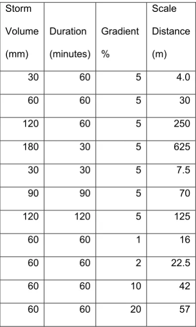
Equation (7) provides an explicit relationship between the runoff coefficient and slope length, for a particular storm, with maximum runoff for short slopes and steadily decreasing as length increases. Figure 9 shows examples of curves obtained for the full simulation, closely conforming to equation (7) and Table 2 shows estimated values of the estimated scale
distance for a range of storms, showing variations over more than two orders of magnitude that vary most strongly with storm total rainfall.
If the scale distance defined here is greater than the length of the slope, then the whole hillslope is contributing significant runoff, and the runoff coefficient begins to increase towards its asymptotic value of 100%. Comparing this approach with the analysis using equation (1), and illustrated in figure 7(b) above, the threshold R0, near which runoff approaches 100%, can be interpreted as the storm rainfall at which the scale distance becomes equal to the slope length, and the fall-off in runoff below that as the effect of reducing scale lengths and associated contributing areas.
with notations as before, except that R0should now be specifically associated with a
particular “standard” slope length L0, in this case the 320 m slope length used in most of the simulations reported here. Combining these equations gives the more general form:
(9)
which combines the two approaches. It follows that, for a given storm rainfall R, the scale distance of connectivity
(10)
and that, for a given slope length L, the associated rainfall threshold parameter
(11).
The simulations presented here suggest that, for a semi arid area, the infiltration excess overland flow at any point depends on the localised convergence of catchment area within the (variable) scale distance of connectivity which depends on storm magnitude. For all but the largest events, flow is generated patchily within a catchment, and the threshold for
This contrasts with behaviour in a humid area, for which the saturated contributing area is loosely related to the topographic index (the ratio of total catchment area to local gradient) and saturation excess overland flow is concentrated on downstream areas of low gradient, with the threshold for contribution primarily set up by antecedent conditions.
Some additional factors and conclusions
(i) Slope profile form
Although it has been seen above that the runoff hydrograph from a simple storm is only secondarily dependent on the plan form of the slope, and that the form of the total infiltration curve conforms to a simple algebraic form with only one changing parameter as storm duration, gradient and overland flow velocity are varied, nevertheless it has been found that there is strong sensitivity to the form of the slope profile. Figure 10 compares the total infiltration curves as storm duration is varied for respectively uniform (figure 10a), convex (b), concave (c) and convexo-concave (d) profiles, all with an average overall profile of 5%. These curves depart somewhat from the form of equation (1) above, perhaps towards
(12)
gradient, with accelerating overland flow, and the increased removal of water from downslope areas after rainfall ceases, again due to the increased gradient and more rapid overland flow. In contrast, profiles with a concave base show slowing of overland flow, so that water remains on the surface for longer, and is able to continue infiltrating. These simulations suggest that slope profile form has a greater control on runoff dynamics than slope plan form, which was seen above to have only a second order effect.
(ii) Coarse-scale estimates of runoff
Alternatives to the use of individual daily rain totals were considered in this analysis. In particular exponentially weighted sums of successive rainfalls were tried, with a range of time decay constants, for both hourly and daily time steps. These measures, that give some weight to antecedent conditions, were. However, only marginally better as predictors of runoff. It is possible that, for a less arid area, such measures might be more advantageous.
In figure 12 (c) an additional curve has been drawn, following the form of equation (1) above, expressed in the appropriate form for total storm runoff (and identifying storm total runoff with daily rainfall totals). Curves have been drawn for a rainfall threshold of R= 70 mm. The criteria used to fit these values were first to fit the general form shown in figure 12(c), particularly for the larger events, and second to provide a correct estimate of the total simulated runoff (using the daily sum aggregated from hourly time steps) over the ten-year period. Values from these estimates based on daily rainfall, using Equation (1), are also shown in figures 12(a) and (b).
(iii) Further dynamic interactions
topography has been adjusted to account for sediment transport after each time step, and the time steps varied dynamically to maintain computational stability. (a) shows the
development of distinct rill-like channels which modify the initial surface, similar to that shown in figure 1 (a) and (d). Figure 12 (b) shows the runoff and sediment response in the first five of these storms. It can be seen that, in accordance with results reported above, the changes in plan form make only minor changes in the amount of runoff, although the
improving network structure allows runoff to peak earlier in each event. However, sediment transport increases greatly as drainage network evolves, eventually levelling off in this example as improved connectivity is compensated by the decreasing gradient at rill outlets (and this is a result of the fixed basal boundary condition used here). These erosional dynamics evolve both within a single storm and over a series of storms, and may in practice be partly countered by tillage operations and natural processes (e.g. Schumm, 1956) that destroy rills between storm events.
A more subtle dynamic process, and one that has not been investigated, may accompany crusting and erosion through the evolution of spatial structural patterns for infiltration parameters. Crusting provides a mechanism for reducing inter-rill infiltration, and selective transportation of material may lead to increases in infiltration rate downstream along rill pathways. Another important process is vegetation change. Growth follows seasonal cycles and responds to the availability of soil moisture through a series of rainfall events, as well as interacting with cultivation, fire and grazing.
(iv) Provisional conclusions
measurements on the scales simulated here, so that the simulations provide a method to explore some of the often complex and contradictory relationships between rainfall and runoff. In particular simulation provides a way of understanding how the effects of gradient, roughness, infiltration capacity and topography in plan and profile are expressed in the rainfall-runoff relationship at a scale that can be incorporated into a catchment model.
References cited
Bartel H., J. Van Nieuwenhuyse, M.Antoine,G. Wyseureand G. Govers, 2011. Pattern-process relationships in surface hydrology: hydrological connectivity expressed in landscape metrics. Hydrological Processes, 25, 3760-3773.
Bracken, L.J. and Croke, J., 2007. The concept of hydrological connectivity and its contribution to understanding runoff-dominated geomorphic systems. Hydrological Processes 21, 1749-1763.
Bracken, L.J., J. Wainwright, G.A. Ali. D. tetzlaff, M.W. Smith, S.M. Reaney, A.G. Roy 2013. Concepts of hydrological connectivity, research approaches, pathways and future agendas. Earth Science Reviews 119, 17-34.
Cammeraat, L.H., 2002. A review of two strongly contrasting geomorphological systems within the context of scale. Earth Surface Processes and Landforms, 27, 1201-1222. Dalen, E.N., 2011. Factors influencing runoff generation, and estimates of runoff in a
semi-arid area, S.E.Spain. Unpublished MPhil thesis, University of Leeds.
Emmett, W.W., 1970. The hydraulics of overland flow in hillslopes. U.S.G.S. Professional Paper 662A, 68pp.
Green, W.H. and G.A. Ampt, 1911.Studies in Soil Physics I. The flow of air and water through soils.
J. Agric Soils, 4, 1- 24.
Holden,J., M. J. Kirkby, S. N. Lane, D. G. Milledge, C. J. Brookes, V. Holden, and A.T. McDonald,
2008. Overland flow velocity and roughness properties in peatlands. Water Resources
Research,. 44, W06415, doi:10.1029/2007WR006052
Kirkby, M.J. 1976. Implications for Sediment Transport, p 325-363 in Kirkby, M.J. (Ed) Hillslope
Lane, S.N., S.M. Reaney, A.C. Heathwaite, 2009. Representation of landscape hydrological
connectivity using a topographically driven surface flow index. Water resources Research 45,
W08423.
McRae, B.H., B.G. Dickson, T.H. keitt, V.B. Shah, 2008. Using Circuit Theory to model connectivity
in ecology, evolution asnd conservation. Ecology 89, 2712-2714.
Mueller, E.N., J. Wainwright, A.J. Parsons, 2008. Spatial variability of soil and nutrient
characteristics of semi-arid grasslands and shrublands, Jornada Basin, New Mexico.
Ecohydrology 1, 3-12.
Philip, J.R., 1957-58. The theory of infiltration. Soil Sci., 83, 345-257; 535-448: 84, 163-177;
257-264: 85, 278-286; 333-337.
Reaney ,S.M., Bracken, L.J. and Kirkby, M.J., 2007. Use of the connectivity of runoff model connectivity in semi-arid areas. Hydrological Processes., 21 (7). 894-906.
Stieglitz, M. J. Shaman, J. Mcnamara, V. Engel, J. Shanley, G.W. Kling, 2003. An approach to
understanding hydrologic connectivity on the hillslope and the implications for nutrient transport.
Global Biogeochemical Cycles 17, 1105, doi:10.1029/2003GB002041
Wainwright, J., A.J. Parsons, E. N. Müller, R.E. Brazier, D. M. Powell and B. Fenti, 2008. A
Transport-Distance Approach to Scaling Erosion Rates: 1. Background and model
development. Earth Surface Processes and Landforms, 33, 813-826.
Wainwright, J., L. Turnbull , T. G. Ibrahim, I. Lexartza-Artza, S. F. Thornton and R. E. Brazier, 2011. Linking environmental régimes, space and time: Interpretations of structural and functional connectivity. Geomorphology, 126, 387-404.
Table 1:
Approximate values of storm response parameter R0, for total runoff at the slope base (320m). For a given total storm rainfall, total storm runoff, r is given by the expression.
The RMS error is calculated by comparing simulated total infiltration (= R-r) with that derived from the expression, for total storm rainfalls of 30,45,60,75,90, 120 & 180mm.
Gradient
(%) Duration (min) ofv rate (sec-1) Infiltration ratio (%) RBest fit 0 (mm)
RMS error
(mm) Associated figure 2% 30 250 100 109 1.15 5% 30 250 100 95 2.39 10% 30 250 100 88 3.41 30% 30 250 100 78 4.71 5% 60 250 100 110 2.24 5% 90 250 100 126 2.08 5% 120 250 100 141 2.17 5% 60 250 50 71 1.57
Table 2. Scale travel distances for infiltration downslope. Storm Volume (mm) Duration (minutes) Gradient % Scale Distance (m)
30 60 5 4.0
60 60 5 30
120 60 5 250
180 30 5 625
30 30 5 7.5
90 90 5 70
120 120 5 125
60 60 1 16
60 60 2 22.5
60 60 10 42
Figure captions
1: Slope surfaces used for 128x128 simulations: contour maps (a-c): catchment areas (d-f).(a) and (d) represent the ‘smoothish’ surface: (b) and € the ‘Rough’ surface; (c) and (f) the ‘valleyed’ surface.
2: Cumulative infiltration values used in simulations, based on field measurements for SE Spain
3: Stages in runoff evolution during and after a rain event (180 mm from times 30-45). Blank areas have no flow.(a) t=34: (b) t=45: (c) t=60: (d) t=100 minutes.
4(a): Example of runoff evolution over time: Hydrographs of slope-base runoff for rainfall at 60mm/hour of differing durations
(b): Example of runoff contributions over space from each section of the slope: 120 mm storm over 60 minutes (intervals 30-60) on planar slope
5.: Total storm runoff (mm) from a 120 mm, 60 minute storm expressed in relation to area drained, at various distances in cells from the divide on (a)the smoothish surface; (b) the valleyed surface
6. Response of simulated overland flow to differences in overland flow velocity parameter (in units of s-1). (a) and (b) show differences in total runoff and with slope position. (c) and (d) show differences in hydrograph form. (a) and (c) are for a 30 mm, 60 minute storm: (b) and (d) for a 120mm, 60 minute storm.
7. Dependence of total slope base storm runoff on storm size for various gradients in simulated 30 minute storms. The results are expressed as (a) Total storm; (b) Runoff coeffieient and (c) total volume infiltrated.
using parameter values shown in Table 1. Legend refers to source of variation within each group.
9. Examples of connectivity relationships between slope length and simulated runoff for 60 minute storms, closely conforming to the form of equation (6)
10. The relationship between simulated total volume infiltrated and storm volume, illustrating the influence of slope profile form and storm duration. (a) Uniform gradient (b) convex profile (c) concave profile (d) convexo-concave profile.
11. Example of runoff contributions over space from each section of the slope for a 120 mm, 60 minute storm (time intervals 30-60) on (a) convex slope, (b)concave slope (c) convexo-concave slope.
12. (a) Simulated runoff for 10-year period of observed rainfall, using hourly and daily time steps. (b) Expansion of simulated runoff for a 20-day storm period within the 10-year period, using hourly and daily time steps. (c) Relationship between daily rainfall totals for 10-year record, and daily sums of simulated hourly runoffs. Curve shows fitted algebraic
expression of equation (1).
13. The impact of repeated 180 mm, 60 minute storms, allowing overland flow and rainsplash to erode the initially smoothish surface. Channelling concentrates the flow, but may also reduce gradients near the channel outlets (a) the surface after erosion by 10 storms. (b)
b)Basal runoff hydrographs and sediment transport for the first six storms. Subsequent storms show similar patterns to the final storm shown here. The initial step increase in sediment at the start of each storm is due to rainsplash.