On the relative sizes of planets within kepler multiple-candidate systems

C

2013. The American Astronomical Society. All rights reserved. Printed in the U.S.A.

ON THE RELATIVE SIZES OF PLANETS WITHIN

KEPLER

MULTIPLE-CANDIDATE SYSTEMS

David R. Ciardi1, Daniel C. Fabrycky2, Eric B. Ford3, T. N. Gautier III4, Steve B. Howell5, Jack J. Lissauer5, Darin Ragozzine3, and Jason F. Rowe5

1_{NASA Exoplanet Science Institute/Caltech, Pasadena, CA 91125, USA;[email protected]} 2_{UCO/Lick Observatory, University of California, Santa Cruz, CA, USA}

3_{Department of Astronomy, University of Florida, Gainesville, FL, USA} 4_{Jet Propulsion Laboratory, Pasadena, CA, USA}

5_{NASA Ames Research Center, Mountain View, CA, USA}

Received 2012 October 8; accepted 2012 November 27; published 2013 January 4

ABSTRACT

We present a study of the relative sizes of planets within the multiple-candidate systems discovered with theKepler mission. We have compared the size of each planet to the size of every other planet within a given planetary system after correcting the sample for detection and geometric biases. We find that for planet pairs for which one or both objects are approximately Neptune-sized or larger, the larger planet is most often the planet with the longer period. No such size–location correlation is seen for pairs of planets when both planets are smaller than Neptune. Specifically, if at least one planet in a planet pair has a radius of3R_⊕, 68%±6% of the planet pairs have the inner planet smaller than the outer planet, while no preferred sequential ordering of the planets is observed if both planets in a pair are smaller than3R_⊕.

Key word: planetary systems

1. INTRODUCTION

Approximately 20% of the planetary candidate systems discovered thus far by Kepler (Borucki et al. 2010) have been identified as having multiple transiting candidate planets (Batalha et al. 2012). As Kepler continues its mission, the number of multiple-planet systems is likely to grow—not only because the total number of systems known to host planets will increase, but also because previously identified “single”-candidate systems may be found to have additional planets not previously detected. For example, 96 (11%) of the “single”-candidate systems from the Borucki et al. (2011)KeplerObject of Interest (KOI) list are now listed on the Batalha et al. (2012) KOI list as having multiple planetary candidates. Thus, understanding planets in multiple systems is not only important for placing into context our own solar system (the best-studied planetary system), but multiple planetary systems may turn out to be the rule rather than the exception.

Typical detailed confirmation of individual planetary systems takes a concerted ground-based observational and modeling effort to rule out false positives caused by blends (e.g., Batalha et al.2011; Torres et al.2011). However, the multiple-candidate systems provide additional information that can be used to confirm planets directly via transit timing variations (Steffen et al.2012a; Fabrycky et al.2012a) or via statistical arguments that multiple transiting systems discovered byKeplerare almost all true planetary systems (Latham et al.2011; Lissauer et al. 2011b,2012). Indeed, based upon orbital stability arguments,

≈96% of the pairs within multiple-candidate systems are most likely real planets around the same star (Fabrycky et al.2012b). The higher statistical likelihood that candidates in multiple systems are true planetary systems has enabled studies of the properties of planetary systems with a lower level of false positive contamination than would be expected if all transiting systems were studied. The overall false positive rate within the Kepler candidate sample has been estimated to be 10%–35% (e.g., Morton & Johnson2011; Santerne et al. 2012), but in comparison, the overall false positive rates among the multiple transiting systems are expected to be1% (Lissauer et al.2012).

The multiple-candidate systems also provide another level of certainty to the studies of planetary systems. The quality of knowledge of planetary characteristics for individual planets often is dependent upon the quality of knowledge of the host stellar characteristics. For example, planetary radii uncertainties for transiting planets are dominated by the uncertainties in the stellar radii (transit depth ∝ (Rp/R)2), and changes in our understanding of the stellar radius can greatly alter our understanding of the radii of individual planets (e.g., Muirhead et al.2012). By studying therelativeproperties of planets within multiple systems, systematic uncertainties associated with the stellar properties are minimized.

Understanding the relative sizes and, hence, the relative bulk compositions and structures of the planets within a system can yield clues on the formation, migration, and evolution of planets within an individual system and on planetary systems as a whole (e.g., Raymond et al. 2012). Within our solar system, the distribution of the unique pairwise radii ratios for each planet compared to the planets in orbits exterior to its orbit (e.g., Mercury–Venus, Mercury–Earth,. . . ,Mercury–Neptune, Venus–Earth, Venus–Mars,. . .etc.) is dominated by ratios less than unity (i.e., the inner planets are smaller than the outer planets). For the eight planets in the solar system, 20 of the 28 (70%) unique radii ratios are<1, but only 3 out of 7 (42%) of neighboring pairs display this sequential size hierarchy. If only the terrestrial planets are considered (Mercury, Venus, Earth, Mars), the fraction is 2/3 with only Mars being smaller than its inner companions.

How the planet sizes are ordered and distributed is likely a direct result of the how the planets formed and evolved. For example, Mars, being the only terrestrial planet in our solar system that does not follow the sequential planet size distribution, may be a direct result of the formation and migration of Jupiter, inward and then back outward leaving a truncated and depleted inner disk out of which Mars was formed (Walsh et al.2011).

around unity, but hints of a planetary size hierarchy can be seen in multi-planet systems discovered byKepler. Kepler-11 has six transiting planets (Lissauer et al. 2011a) with the smallest planets residing preferentially inside the orbits of larger planets. Kepler-11 displays an anti-correlation between the mean density of the planets and the semimajor axis distance from the host star; i.e., the larger and lower density planets are located farther out than the smaller and denser planets, possibly indicative of the formation and/or evolution of the planetary system (Migaszewski et al.2012). Kepler-47, the only known circumbinary multiple-planet system, also displays a size hierarchy with the inner planet (∼3R_⊕) being smaller than the outer planet (∼4.6R_⊕; Orosz et al. 2012). Yet, in Kepler-20 (a five-planet system), the relative sizes of the planets do not appear to correlate with the orbital periods of the planets (Gautier et al.2012; Fressin et al. 2012). But these are only three systems. Is there an overall correlation of planetary size with orbital period?

Here, we explore therelativesizes of the planetary radii for all planet pairs within the multiple-candidate systems discovered thus far by Kepler (Batalha et al. 2012). In this work, we refer to theKeplercandidates as “planets” though the majority have not been formally validated or confirmed as planets; as discussed above, candidates in multiple-candidate systems are statistically more likely to be true planetary systems (Latham et al.2011; Lissauer et al.2011b,2012). We seek to characterize the planetary size hierarchy, as a function of the number of planets detected in the systems and the properties of the stellar hosts, and explore if the size hierarchy seen within the inner solar system also occurs in theKeplermultiple-candidate sample.

2. THE SAMPLE

The sample used here is based upon the 2012 KOI candidate list published by Batalha et al. (2012); a full description of the KOI list, the vetting that list underwent, and the characteristics of the sample set as a whole are described in the catalog paper. There are 1425 systems with a single candidate, 245 systems with two planet candidates, 84 systems with three planet candidates, 27 systems with four planet candidates, 8 systems with five planet candidates, and 1 system with six planet candidates. Here we wish to investigate the overall distribution of planet sizes as a function of orbit; that is, do outer planets, in general, tend to be larger than inner planets?

A smaller planet (e.g., shallower transit) will be more easily detected if the period is short, simply from the fact that the number of observed transiting events increases with shorter orbital period. In a complementary manner, the larger planets are more easily detected at all periods, up to some period threshold where only 2–3 transits are detected. Batalha et al. (2012) tabulate for each candidate the transit period, the transit duration, the impact parameter, and the signal-to-noise ratio (S/N) of the transit fits. The S/Ns, coupled with the transit periods and the impact parameters, enable us to debias the sample for these observational detection efficiencies (see also Lissauer et al.2011b).

The multiple-candidate systems were identified primarily by searching the single-candidate systems specifically for addi-tional transiting planets. Thus, there could potentially be a de-tection bias of which we are unaware that is not found in the single-candidate systems. However, no substantial difference between single-planet systems and the multiple-planet systems was found, except for the lack of hot Jupiters in the multiple-planet systems (Latham et al.2011; Steffen et al.2012b). The

Figure 1.Distribution of the transit signal-to-noise ratio for all the detected “multiple” candidates from Batalha et al. (2012). The solid curve is an exponential fit to the S/N distribution, and the vertical dashed line at S/N=25 marks approximately where the exponential no longer adequately describes the distribution (see inset figure).

overall size distribution of the planets and the S/N detection thresholds appear to be similar between the single-candidate and multiple-candidate systems.

To understand better the detection thresholds for the multiple-candidate systems, we have used the distribution of the total transit S/N to estimate where the distribution of planets in multiple systems appears to be complete (Figure1). Assuming the S/N distribution can be characterized with an exponential function where the distribution is complete, we have used the point in the S/N distribution function where the exponential no longer adequately describes the distribution as the fiducial for completeness. Fitting the exponential, we find a turnover in detected samples at an S/N ≈25. We use this S/N threshold to debias the radii–ratio distribution of planets in multiple-candidate systems.

The total S/N of all the detected transits for each planetary candidate is predicted for all the observed orbital periods within a system. A planet pair is retained in the analysis only if the predicted total transit S/Ns for both planets at the orbital period of the other planet exceeds the S/N threshold of S/N>25. The predicted S/N is determined by scaling the measured total S/N of the planet transits by the ratio of the orbital periods. Assuming all else is equal, the total S/N of all the detected transits for a given planet scales with the orbital period asP−1/3_.

For a given planet, the total S/N of all detected transits is proportional to the total number of points (n) detected in all of the transits (e.g., von Braun et al.2009)

(S/N)transits∝(n)1/2∝(N·nt)1/2, (1)

where N is the total number of individual transits detected, andntis the number of points detected within a single transit. The number of transits detected is inversely proportional to the orbital period (N ∝ 1/P), and the number of points detected per transit is proportional to the transit duration (nt ∝tdur); thus, the total S/N of the detected transits can be parameterized as

(S/N)transits∝(tdur/P)1/2. (2)

The transit duration (t_dur) is proportional to the cube root of the orbital period (tdur ∝ v−orb1 ∝ P1

Figure 2.Distributions of the radii and orbital periods of the planets that are used in this study. The vertical dashed lines mark the median values of the distributions.

detected transits scales with the orbital period as

(S/N)transits∝(P1/3/P)1/2∝P−1/3. (3)

An additional restriction on the sample was made such that no planet candidate was included that has an impact parameter of

b0.8. At such high impact parameters, the transit parameters, particularly the transit depth (i.e., the planet radius), are less certain. Using the S/N>25 detection threshold and the impact parameter restrictions, there are 96 multiple-candidate systems with 159 pairs of planets (228 individual planets) in the analysis. All of the planet pairs used in the analysis of this paper are summarized in Table1; planets are labeled with roman numerals (I, II, III, IV, V, VI) in the order of increasing orbital period. These do not necessarily correspond to KOI fraction numbers (e.g., .01, .02, ...) nor do they correspond to the confirmed planet letters (e.g., Kepler-11b, Kepler-11c, ...). After the S/N and impact parameter cuts, the largest planet in the sample is 13R_⊕, and the median planet radius is≈2.5R_⊕; the smallest planet retained in the sample has a radius of 0.75R_⊕. The orbital periods of the planets in this sample span 0.45–331 days, with an median period of∼13.1 days. The distributions of the radii and orbit periods for the 228 planets retained in the sample are shown in Figure2.

Previous work indicates that the detected planets in theKepler multiple-candidate systems have mutual inclinations of 1◦–3◦ (Fabrycky et al.2012b; Fang & Margot2012). Due to the usual limitation of the transit technique in only detecting planets that are very nearly edge-on, theKepler sample used here is naturally biased to systems of nearly coplanar planets. The prevalence of Kepler multiple-candidate systems shows that

Figure 3. Observed cumulative distribution of the planet-radii ratios for all planet pairs (black histogram), and the predicted cumulative distribution for planet radii drawn randomly from the measure planet sample (gray histogram). The horizontal dot-dash line marks the fraction of planet pairs with Rinner/Router < 1; the gray region marks the 1σ confidence interval for this fraction. The vertical dashed line marks the boundary whereRinner/Router=1, and the horizontal dashed line marks the 50% fraction.

there is a large population of such systems with small planets and orbital periods of tens of days (Figure 2). It may be that other system architectures with higher mutual inclinations or different period ranges do not show the same trend in planet sizes that we describe herein.

3. DISCUSSION

We have calculated the ratios of the inner planet radius to the outer planet radius for each unique pair of planets within a system (Rinner/Router), and the cumulative fraction distribution is displayed in Figure 3. If there were no preference for the ordering of planet sizes, the chance that a given planet-radii ratio is larger than unity would be equal to the chance that the ratio is below unity, and the cumulative fraction distribution would pass through 50% at log(Rinner/Router)=0 (Rinner/Router =1).

In contrast, 59.7+4.1

−4.2% of the planet pairs are ordered such that the outer planet is larger than the inner planet (Rinner/Router <1). The resulting fraction deviates from the null-hypothesis expec-tation value of 50% by≈2.5σ. The 1σ upper and lower confi-dence intervals are based upon the Clopper–Pearson binomial distribution confidence interval (Clopper & Pearson1934). The Clopper–Pearson interval is a two-sided confidence interval and is based directly on the binomial distribution rather than an ap-proximation to the binomial distribution. We do caution that in applying the Clopper–Pearson confidence interval there is an implicit assumption that all elements of the sample are uncorre-lated. Given that not all planet pairs are from independent stellar systems, there may be a correlation between individual planet pairs within a system (i.e., planet I is smaller than planet III because it is smaller than planet II), and the Clopper–Pearson confidence intervals may underestimate the true uncertainties in the fractions.

Table 1

Summary of Planet-radii Ratios

KOI Stellar Planet Inner Planet Outer Planet Planet-radii

Temperature Pair Radius Period Transit Impact Radius Period Transit Impact Ratio

(K) (R_⊕) (days) S/N Par. (R_⊕) (days) S/N Par. Rinner/Router

KOIs with Two Candidates

K00072 5627 I/II 1.38 0.837 139 0.17 2.19 45.294 122 0.11 0.630

K00108 5975 I/II 2.94 15.965 84 0.79 4.45 179.600 111 0.62 0.661

K00119 5380 I/II 3.76 49.184 152 0.55 3.30 190.310 63 0.69 1.139

K00123 5871 I/II 2.64 6.482 98 0.56 2.71 21.222 78 0.01 0.974

K00150 5538 I/II 2.63 8.409 106 0.73 2.73 28.574 81 0.76 0.963

K00209 6221 I/II 5.44 18.795 217 0.51 8.29 50.790 287 0.40 0.656

K00222 4353 I/II 2.03 6.312 85 0.71 1.66 12.794 43 0.72 1.223

K00223 5128 I/II 2.52 3.177 90 0.78 2.27 41.008 32 0.69 1.110

K00271 6169 I/II 2.48 29.392 72 0.71 2.60 48.630 54 0.79 0.954

K00275 5795 I/II 1.95 15.791 55 0.03 2.04 82.199 27 0.60 0.956

K00312 6158 I/II 1.91 11.578 41 0.70 1.84 16.399 40 0.58 1.038

K00313 5348 I/II 1.61 8.436 54 0.32 2.20 18.735 55 0.73 0.732

K00386 5969 I/II 3.25 31.158 57 0.02 2.94 76.732 28 0.55 1.105

K00413 5236 I/II 2.75 15.228 52 0.67 2.10 24.674 26 0.65 1.310

K00431 5249 I/II 2.80 18.870 60 0.60 2.48 46.901 34 0.68 1.129

K00433 5237 I/II 5.60 4.030 127 0.65 12.90 328.240 158 0.77 0.434

K00446 4492 I/II 1.76 16.709 33 0.62 1.72 28.551 34 0.05 1.023

K00448 4264 I/II 1.77 10.139 56 0.74 2.31 43.608 66 0.66 0.766

K00464 5362 I/II 2.63 5.350 75 0.58 6.73 58.362 263 0.20 0.391

K00475 5056 I/II 2.04 8.181 37 0.58 2.26 15.313 34 0.68 0.903

K00509 5437 I/II 2.24 4.167 45 0.09 2.68 11.463 32 0.74 0.836

K00518 4565 I/II 2.11 13.981 68 0.71 1.54 44.000 33 0.49 1.370

K00638 5722 I/II 3.60 23.636 53 0.02 3.78 67.093 39 0.27 0.952

K00657 4632 I/II 1.63 4.069 43 0.63 2.08 16.282 46 0.74 0.784

K00672 5524 I/II 2.60 16.087 43 0.71 3.15 41.749 70 0.11 0.825

K00676 4367 I/II 2.56 2.453 255 0.70 3.30 7.972 348 0.57 0.776

K00693 6121 I/II 1.87 15.660 48 0.50 1.76 28.779 23 0.64 1.062

K00708 6036 I/II 1.82 7.693 43 0.74 2.54 17.406 68 0.70 0.717

K00800 5938 I/II 3.27 2.711 48 0.76 3.39 7.212 36 0.77 0.965

K00841 5399 I/II 5.44 15.334 83 0.74 7.05 31.331 117 0.74 0.772

K00842 4497 I/II 2.04 12.718 43 0.31 2.46 36.065 44 0.42 0.829

K00853 4842 I/II 2.38 8.204 48 0.12 1.78 14.496 22 0.02 1.337

K00870 4590 I/II 2.52 5.912 56 0.76 2.35 8.986 47 0.73 1.072

K00877 4500 I/II 2.42 5.955 54 0.73 2.37 12.039 36 0.79 1.021

K00896 5190 I/II 3.22 6.308 68 0.52 4.52 16.239 91 0.57 0.712

K00936 3684 I/II 1.54 0.893 72 0.75 2.69 9.468 96 0.76 0.572

K00951 4767 I/II 3.74 13.197 101 0.39 2.87 33.653 36 0.58 1.303

K00988 5218 I/II 2.20 10.381 67 0.02 2.17 24.570 37 0.67 1.014

K01236 6562 I/II 2.04 12.309 40 0.01 3.02 35.743 64 0.37 0.675

K01270 5145 I/II 2.19 5.729 45 0.58 1.55 11.609 22 0.01 1.413

K01781 4977 I/II 1.94 3.005 81 0.19 3.29 7.834 172 0.01 0.590

K01824 5978 I/II 1.75 1.678 53 0.70 1.97 3.554 50 0.69 0.888

KOIs with Three Candidates

K00085 6172 I/II 1.27 2.155 72 0.71 2.35 5.860 154 0.77 0.540

K00085 6172 I/III 1.27 2.155 72 0.71 1.41 8.131 53 0.78 0.901

K00085 6172 II/III 2.35 5.860 154 0.77 1.41 8.131 53 0.78 1.667

K00111 5711 I/II 2.14 11.427 96 0.53 2.05 23.668 71 0.55 1.044

K00111 5711 I/III 2.14 11.427 96 0.53 2.36 51.756 75 0.57 0.907

K00111 5711 II/III 2.05 23.668 71 0.55 2.36 51.756 75 0.57 0.869

K00115 6202 II/III 3.33 5.412 144 0.43 1.88 7.126 41 0.55 1.771

K00137 5385 I/II 1.82 3.505 44 0.71 4.75 7.641 299 0.50 0.383

K00137 5385 I/III 1.82 3.505 44 0.71 6.00 14.858 305 0.72 0.303

K00137 5385 II/III 4.75 7.641 299 0.50 6.00 14.858 305 0.72 0.792

K00152 6187 I/II 2.59 13.484 58 0.34 2.77 27.402 57 0.07 0.935

K00152 6187 I/III 2.59 13.484 58 0.34 5.36 52.091 158 0.00 0.483

K00152 6187 II/III 2.77 27.402 57 0.07 5.36 52.091 158 0.00 0.517

K00156 4619 I/II 1.18 5.188 38 0.53 1.60 8.041 54 0.64 0.738

K00156 4619 I/III 1.18 5.188 38 0.53 2.53 11.776 131 0.69 0.466

K00156 4619 II/III 1.60 8.041 54 0.64 2.53 11.776 131 0.69 0.632

K00284 5925 I/II 1.09 6.178 32 0.38 1.14 6.415 35 0.19 0.956

Table 1

(Continued)

KOI Stellar Planet Inner Planet Outer Planet Planet-radii

Temperature Pair Radius Period Transit Impact Radius Period Transit Impact Ratio

(K) (R⊕) (days) S/N Par. (R⊕) (days) S/N Par. Rinner/Router

K00343 5744 I/III 1.86 2.024 72 0.63 1.58 41.809 20 0.53 1.177

K00343 5744 II/III 2.68 4.762 108 0.63 1.58 41.809 20 0.53 1.696

K00351 6103 II/III 6.62 210.590 144 0.22 9.32 331.640 211 0.19 0.710

K00377 5777 II/III 8.28 19.273 136 0.35 8.21 38.907 81 0.62 1.009

K00398 5101 I/II 1.76 1.729 37 0.24 3.33 4.180 102 0.00 0.529

K00398 5101 II/III 3.33 4.180 102 0.00 8.66 51.846 215 0.66 0.385

K00408 5631 I/II 3.72 7.382 96 0.79 2.91 12.560 52 0.77 1.278

K00408 5631 I/III 3.72 7.382 96 0.79 2.70 30.827 34 0.79 1.378

K00408 5631 II/III 2.91 12.560 52 0.77 2.70 30.827 34 0.79 1.078

K00481 5227 I/II 1.54 1.554 43 0.71 2.37 7.650 56 0.76 0.650

K00481 5227 II/III 2.37 7.650 56 0.76 2.44 34.260 39 0.73 0.971

K00528 5448 I/III 2.62 9.577 55 0.48 3.27 96.671 32 0.71 0.801

K00620 5803 I/III 7.05 45.155 132 0.03 9.68 130.180 279 0.06 0.728

K00658 5676 I/II 2.03 3.163 68 0.53 2.02 5.371 52 0.65 1.005

K00658 5676 I/III 2.03 3.163 68 0.53 1.14 11.329 17 0.01 1.781

K00665 5864 I/II 1.16 1.612 34 0.69 1.09 3.072 27 0.64 1.064

K00701 4807 I/II 1.27 5.715 55 0.46 1.95 18.164 71 0.66 0.651

K00701 4807 II/III 1.95 18.164 71 0.66 1.57 122.390 34 0.29 1.242

K00711 5502 II/III 3.18 44.699 51 0.61 2.83 124.520 35 0.49 1.124

K00718 5788 I/II 2.57 4.585 67 0.34 3.06 22.714 58 0.29 0.840

K00718 5788 I/III 2.57 4.585 67 0.34 2.67 47.904 27 0.68 0.963

K00718 5788 II/III 3.06 22.714 58 0.29 2.67 47.904 27 0.68 1.146

K00723 5244 I/III 3.26 3.937 72 0.79 3.61 28.082 60 0.58 0.903

K00757 4956 I/II 2.09 6.253 34 0.00 4.73 16.068 120 0.25 0.442

K00757 4956 II/III 4.73 16.068 120 0.25 3.21 41.192 40 0.35 1.474

K00806 5461 II/III 13.24 60.322 366 0.37 9.52 143.210 69 0.34 1.391

K00864 5337 I/III 2.51 4.312 63 0.14 2.23 20.050 30 0.00 1.126

K00884 4931 II/III 4.13 9.439 143 0.48 4.23 20.476 73 0.70 0.976

K00898 4648 I/II 2.18 5.170 35 0.64 2.83 9.771 47 0.68 0.770

K00898 4648 II/III 2.83 9.771 47 0.68 2.36 20.089 28 0.59 1.199

K00921 5046 II/III 2.66 10.281 43 0.69 3.09 18.119 46 0.70 0.861

K00941 4998 I/II 2.37 2.383 38 0.53 4.14 6.582 99 0.03 0.572

K00961 4188 I/II 2.63 0.453 100 0.69 2.86 1.214 73 0.77 0.920

K01576 5445 I/II 3.20 10.415 64 0.68 2.84 13.084 50 0.65 1.127

K01835 5004 I/II 2.69 2.248 43 0.44 3.11 4.580 37 0.67 0.865

K01860 5708 II/III 2.44 6.319 46 0.46 2.36 12.209 36 0.35 1.034

K01867 3892 I/II 1.21 2.549 37 0.40 1.08 5.212 25 0.31 1.120

KOIs with Four Candidates

K00094 6217 I/II 1.41 3.743 35 0.16 3.43 10.423 78 0.01 0.411

K00094 6217 II/III 3.43 10.423 78 0.01 9.25 22.343 455 0.30 0.371

K00094 6217 II/IV 3.43 10.423 78 0.01 5.48 54.319 206 0.38 0.626

K00094 6217 III/IV 9.25 22.343 455 0.30 5.48 54.319 206 0.38 1.688

K00191 5495 II/III 2.25 2.418 53 0.55 10.67 15.358 642 0.59 0.211

K00191 5495 III/IV 10.67 15.358 642 0.59 2.22 38.651 21 0.52 4.806

K00245 5288 II/III 0.75 21.301 49 0.76 2.00 39.792 282 0.79 0.375

K00571 3881 I/II 1.31 3.887 36 0.76 1.53 7.267 36 0.76 0.856

K00571 3881 II/III 1.53 7.267 36 0.76 1.68 13.343 36 0.79 0.911

K00571 3881 II/IV 1.53 7.267 36 0.76 1.53 22.407 27 0.78 1.000

K00571 3881 III/IV 1.68 13.343 36 0.79 1.53 22.407 27 0.78 1.098

K00720 5123 I/II 1.41 2.796 58 0.08 2.66 5.690 124 0.40 0.530

K00720 5123 I/III 1.41 2.796 58 0.08 2.53 10.041 87 0.64 0.557

K00720 5123 II/III 2.66 5.690 124 0.40 2.53 10.041 87 0.64 1.051

K00733 5038 II/III 2.54 5.925 60 0.14 2.21 11.349 35 0.31 1.149

K00812 4097 I/III 2.19 3.340 54 0.13 2.11 20.060 28 0.35 1.038

K00834 5614 III/IV 1.98 13.233 33 0.38 5.33 23.653 154 0.38 0.371

K00869 5085 II/IV 2.73 7.490 43 0.47 3.20 36.280 34 0.42 0.853

K00880 5512 III/IV 4.00 26.442 48 0.64 5.35 51.530 109 0.02 0.748

K00952 3911 II/III 2.25 5.901 47 0.72 2.15 8.752 35 0.77 1.047

K00952 3911 II/IV 2.25 5.901 47 0.72 2.64 22.780 38 0.77 0.852

K00952 3911 III/IV 2.15 8.752 35 0.77 2.64 22.780 38 0.77 0.814

K01557 4783 II/IV 3.60 3.296 122 0.52 3.01 9.653 70 0.30 1.196

K01567 5027 II/III 2.46 7.240 34 0.36 2.22 17.326 23 0.00 1.108

Table 1

(Continued)

KOI Stellar Planet Inner Planet Outer Planet Planet-radii

Temperature Pair Radius Period Transit Impact Radius Period Transit Impact Ratio

(K) (R⊕) (days) S/N Par. (R⊕) (days) S/N Par. Rinner/Router

K01930 5897 II/IV 2.21 13.726 38 0.60 2.46 44.431 29 0.66 0.898

K01930 5897 III/IV 2.14 24.310 31 0.62 2.46 44.431 29 0.66 0.870

KOIs with Five Candidates

K00070 5443 I/II 1.92 3.696 134 0.60 0.91 6.098 23 0.66 2.110

K00070 5443 I/III 1.92 3.696 134 0.60 3.09 10.854 260 0.55 0.621

K00070 5443 I/IV 1.92 3.696 134 0.60 1.02 19.577 18 0.74 1.882

K00070 5443 I/V 1.92 3.696 134 0.60 2.78 77.611 103 0.55 0.691

K00070 5443 III/V 3.09 10.854 260 0.55 2.78 77.611 103 0.55 1.112

K00082 4908 III/IV 1.29 10.311 79 0.71 2.45 16.145 172 0.73 0.527

K00082 4908 III/V 1.29 10.311 79 0.71 1.03 27.453 28 0.79 1.252

K00082 4908 IV/V 2.45 16.145 172 0.73 1.03 27.453 28 0.79 2.379

K00232 5868 I/II 1.73 5.766 41 0.40 4.31 12.465 207 0.43 0.401

K00232 5868 I/III 1.73 5.766 41 0.40 1.69 21.587 21 0.67 1.024

K00232 5868 II/III 4.31 12.465 207 0.43 1.69 21.587 21 0.67 2.550

K00232 5868 II/IV 4.31 12.465 207 0.43 1.79 37.996 21 0.56 2.408

K00232 5868 II/V 4.31 12.465 207 0.43 1.69 56.255 19 0.38 2.550

K00500 4613 III/IV 1.63 4.645 30 0.72 2.64 7.053 59 0.71 0.617

K00500 4613 IV/V 2.64 7.053 59 0.71 2.79 9.522 55 0.79 0.946

K00707 5904 II/III 3.42 13.175 37 0.77 5.69 21.775 80 0.77 0.601

K00707 5904 II/IV 3.42 13.175 37 0.77 4.26 31.784 42 0.77 0.803

K00707 5904 II/V 3.42 13.175 37 0.77 4.77 41.029 51 0.77 0.717

K00707 5904 III/IV 5.69 21.775 80 0.77 4.26 31.784 42 0.77 1.336

K00707 5904 III/V 5.69 21.775 80 0.77 4.77 41.029 51 0.77 1.193

K00707 5904 IV/V 4.26 31.784 42 0.77 4.77 41.029 51 0.77 0.893

K01589 5755 II/III 2.23 8.726 30 0.72 2.36 12.882 27 0.79 0.945

KOIs with Six Candidates

K00157 5685 I/II 1.89 10.304 38 0.34 2.92 13.024 67 0.35 0.647

K00157 5685 I/III 1.89 10.304 38 0.34 3.20 22.686 73 0.33 0.591

K00157 5685 I/IV 1.89 10.304 38 0.34 4.37 31.995 87 0.79 0.432

K00157 5685 II/III 2.92 13.024 67 0.35 3.20 22.686 73 0.33 0.913

K00157 5685 II/IV 2.92 13.024 67 0.35 4.37 31.995 87 0.79 0.668

K00157 5685 II/V 2.92 13.024 67 0.35 2.60 46.687 40 0.49 1.123

K00157 5685 II/VI 2.92 13.024 67 0.35 3.43 118.360 54 0.36 0.851

K00157 5685 III/IV 3.20 22.686 73 0.33 4.37 31.995 87 0.79 0.732

K00157 5685 III/V 3.20 22.686 73 0.33 2.60 46.687 40 0.49 1.231

K00157 5685 III/VI 3.20 22.686 73 0.33 3.43 118.360 54 0.36 0.933

K00157 5685 IV/V 4.37 31.995 87 0.79 2.60 46.687 40 0.49 1.681

K00157 5685 IV/VI 4.37 31.995 87 0.79 3.43 118.360 54 0.36 1.274

K00157 5685 V/VI 2.60 46.687 40 0.49 3.43 118.360 54 0.36 0.758

Table 2

Planet-radii Ratios Summary Grouped by Number of KOIs

All 2-KOI 3-KOI 4-KOI 5-KOI 6-KOI

Systems Systems Systems Systems Systems Systems

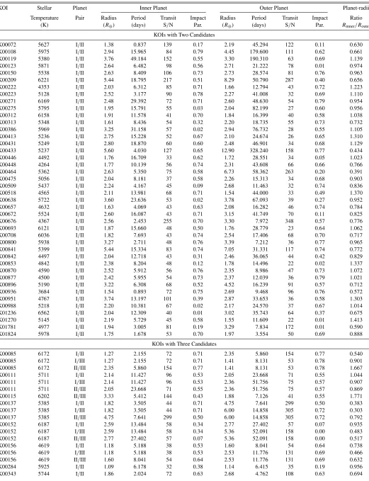
No. of stellar systems 96 42 33 14 6 1

No. ofRinner/Routerpairs 159 42 55 27 22 13

No. ofRinner/Router<1 95 26 33 16 11 9

No. ofRinner/Router>1 64 16 22 11 11 4

χ2statistica 6.0 2.4 2.2 0.93 0.0 1.9

χ2probabilitya 0.014 0.13 0.14 0.34 1.0 0.16

FractionRinner/Router<1 0.597 0.619 0.600 0.592 0.500 0.692

Lower 1σconfidence 0.042 0.089 0.076 0.115 0.126 0.179

Upper 1σconfidence 0.041 0.082 0.072 0.107 0.126 0.140

Note.aTheχ2statistic and probability are based upon comparison of the observed fractions to the null hypothesis fractions of 50%. We also have performed three additional observational tests

to assess if the observed fraction may be the result of an unrecognized bias in the sample. The first test repeated the above analysis, but for each unique planet pair, the measured

Figure 4.Observed fraction of planet pairs withRinner/Router <1 is plotted as a function of signal-to-noise cutoff, showing the fraction asymptotically approaches the a value of ∼0.6 for S/N 20. The dashed line marks the observed fraction (and the 1σ confidence interval; dotted lines) for an S/Nthreshold=25 (from Figure3).

were applied (e.g., if a planet radius was drawn that was too small to be detected at the orbital period (S/N < 25), a new radius was randomly drawn until the S/N threshold was met). The random draw was performed 10,000 times for each unique pair of planets, and the cumulative distribution of the planet-radii ratios for all of the random draws is displayed in Figure3. As expected, the random draw distribution displays no size ordering preference; i.e., the fraction of planets with

Rinner/Router<1 is≈50%. Based upon a Kolmogorov–Smirnov test, the observed distribution and the random draw distribution are not drawn from different parent distributions with only a probability of 3×10−8_{—indicating that the observed} planet-radii ratio distribution has a preferential ordering such that smaller planets are in orbits interior to larger planets.

We also tested if the observed fraction of planet-radii ratios withRinner/Router < 1 is dependent upon the S/N threshold chosen. In Figure4, the fraction of planet pairs where the inner planet is smaller than the outer planet is plotted as a function of the required S/N threshold. If no S/N threshold is required, the fraction is>70%, and as the S/N threshold is increased, the fraction systematically decreases and levels out near∼60%. The higher fractions at a lower S/N threshold result from incompleteness of the sample (i.e., it is easier to detect larger planets at all orbital periods). As the S/N threshold is increased the fraction of planet-radii ratios below unity decreases, but does not systematically approach 50%, as would be expected if there were no preferential size ordering of the planets. Rather, the fraction asymptotically approaches 60% for S/N_threshold >20, indicating that the S/N_threshold =25 threshold ensures that the analysis presented in Figure 3 is based upon a sample not significantly biased by completeness.

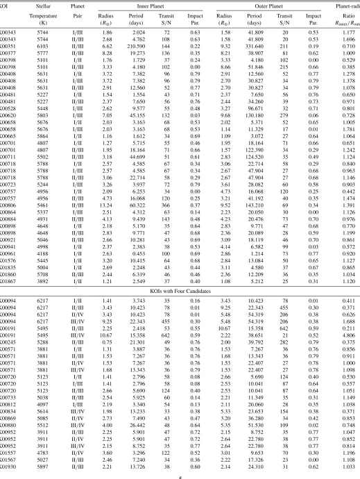
The final test performed was to determine if the observed frac-tion is dependent upon the maximum period of the outer planet (see Figure5). Transit surveys are typically more complete at shorter orbit periods, and if there truly was no preference for planet size ordering, the fraction would decline and approach 50% as the maximum orbit period was decreased. Within the confidence intervals, the observed fractions are independent of the maximum outer orbital period and are consistent with the observed≈60% fraction for the entire sample. The fractions do not approach 50% at shorter orbital period as would be expected

Figure 5.Observed fraction of planet pairs withRinner/Router <1 is plotted as a function of maximum outer orbital period cutoff, showing the fraction asymptotically approaches the value of∼0.6 forP 20. The dashed line marks the observed fraction for the whole sample; the dotted lines mark the 1σ confidence interval (from Figure3). The numbers above each data point indicate the number of planet pairs that appear in that period bin (Pouter< Pmax).

for a random distribution. In fact, a slight (but not statistically significant) hint of a higher fraction is observed if the maximum period isP <20 days.

Overall, if the ordering of planets within a given system was random such that there was no sequential ordering of the planets by size, the probabilities of a planet-radii ratio being above or below unity would be equal. But that is not what is observed; the three tests above (i.e., the random radius draw, the S/N_threshold, and the maximum outer orbital period), in combination with the

χ2_{probability statistic and the confidence intervals, indicate that} for≈60% (2.5σ) of the unique planet pairs within theKepler multiple-planet systems, the inner planet is smaller than the outer planet, with only a 1.4% chance of this being observed by chance. In the following subsections, we explore if and how the number of planets in the system, the orbital separation of the planets, the temperature of the stars, and the size of the planets themselves may affect the observed size hierarchy of the planets in multiple-planet systems.

3.1. The Number of Planets and Orbital Separation

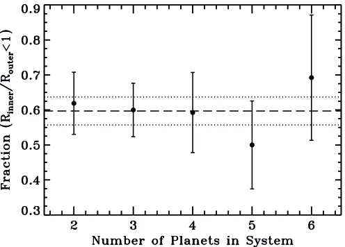
If formation and evolutionary mechanisms within a planetary system affect the size distribution and ordering of planets within a system, one might expect to observe differences in the size ordering as a function of the number of planets within a system. When the planets are divided into groups based upon the number of detected planetary candidates in the system (e.g., two-, three-, four-, five-, and six candidates), the fractions do not change appreciably from the fractions calculated for the entire sample set. This can be seen in both theχ2 statistic (Table2) where theχ2_{and associated probabilities are all comparable to} each other and in Figure6, where the observed fractions (with confidence intervals) are plotted and display no dependence on the number of planets in the system. While the number of systems with more than three planets have relatively large uncertainties and poor statistics because of the small numbers of the four-, five-, and six-candidate systems, there is no correlation of the fraction of size-ordered planets with the number of planets within a planetary system.

Figure 6.Observed fraction of planet pairs with the inner planet being smaller than the outer planet plotted as a function of the number of KOIs within a system. The dashed line marks the observed fraction for the whole sample; the dotted lines mark the 1σconfidence interval (from Figure3).

at longer orbital periods and, thus, the relative sizes of the planets would be more extreme if the planets are more widely separated (larger orbital period ratio). To test this, we have plotted the planet-radii ratios versus the orbital period ratios and the inner and outer planet orbital periods (Figure7). Using the Spearman non-parametric rank correlation function, we find that the distributions are likely uncorrelated. The correlation coefficients for the three distributions shown in Figure 7 are 0.14, 0.22, and 0.10 with probabilities to be exceeded in the null hypothesis of 0.06, 0.004, and 0.08, respectively.

Additionally, to search for a non-zero slope that might indicate the planet-radii ratios are related to or dependent upon the period or period spacings, we have fitted a linear model6 _{to each} of the distributions. Each of the distributions are statistically consistent with a flat distribution as a function of period ratio and orbital period; the slopes of the fitted linear models were found to be 0.29±0.15 for the radii ratios versus period ratios (Figure 7 top), 0.0009±0.001 for the radii ratios versus the inner orbital period (Figure7middle), and−0.0002±0.0005 for the radii ratios versus the outer orbital period (Figure 7 bottom). In general, we find no correlation between the orbital period separation (or orbital periods themselves) and the size ordering of the planets.

3.2. Stellar Temperature

We have also explored whether there is a correlation be-tween the distribution of planet-radii ratios and the effective temperature of the host stars. We have produced planet-radii ratio distributions, but separated out by the stellar temperature. We chose temperature ranges that roughly correspond to the spectral classification of M- and K-stars (<5000 K), G-stars (5000–5800 K), and F-stars (>5800 K; Ciardi et al.2011). The cumulative distributions of the planet-radii ratios for each of the stellar temperature groups are displayed in Figure8.

Overall, all three distributions are shifted to lower ratios in comparison to the random draw distribution from Figure 3. Kolmogorov–Smirnov tests between the three distributions indicate that the three distributions do not result from different parent distributions with probabilities of >75%, indicating

6 _{Fitting was done with an outlier resistant linear regression routine based} upon Numerical Recipes (Press et al.2007).

Figure 7.Top: distribution of the planet-radii ratios as a function of the orbital period ratio. Middle: distribution of the planet-radii ratio as a function of the inner planet orbital period. Bottom: distribution of the planet-radii ratio as a function of the outer planet orbital period. In each panel, the horizontal dashed line marks unity, and the dot-dashed line delineates the median planet-radii ratio of 0.91 for the entire sample.

that, in general, the preferential planet size ordering occurs at approximately the same level (i.e.,≈60% of the unique planet pairs haveRinner/Router<) across the stellar temperature range. A summary of the planet-radii ratios, the fraction of ratios that exhibit smaller inner planets, and the significance of those fractions based upon the confidence intervals andχ2_{statistic is} given in Table3for each of the stellar temperature groups.

Figure 8.Top: observed cumulative distributions of the planet-radii ratios as displayed in Figure3, except the distributions have been separated out by stellar effective temperature and identified by the plot colors (as labeled in the plot). The plot markings are the same as those in Figure3. Bottom: cumulative distributions of the individual radii for the planets that are used to determine the planet-radii ratios throughout the paper, separated out by stellar effective temperature (as labeled in the plot).

Table 3

Planet-radii Ratios Grouped by Stellar Temperature

>5800 K 5000–5800 K <5000 K

Stars Stars Stars

No. of stellar systems 22 47 27

No. ofRinner/RouterPairs 40 79 40

No. ofRinner/Router<1 26 47 22

No. ofRinner/Router>1 14 32 18

χ2statistic 3.6 2.9 0.4

χ2_{probability 0.06 0.09 0.50}

FractionRinner/Router<1 0.650 0.594 0.550

Lower 1σconfidence 0.091 0.062 0.091

Upper 1σconfidence 0.082 0.060 0.088

Median planet radius (R_⊕) 2.59 2.63 2.19

Med. abs. dev. (R_⊕) 1.49 1.18 0.61

Min. planet radius (R_⊕) 1.09 0.75 1.03

Max. planet radius (R_⊕) 9.68 13.2 4.73

with the higher luminosity stars or perhaps could result from the warmer (i.e., more massive) stars tending to contain larger (i.e., more massive) planets (see Figure8and Table3).

The median planet radius does not vary significantly between the three stellar groups (2.2–2.6R_⊕; see Table3), but the size of the largest planets in each group does. The G and F stars (Teff >5000 K) contain Saturn-sized and Jupiter-sized planets

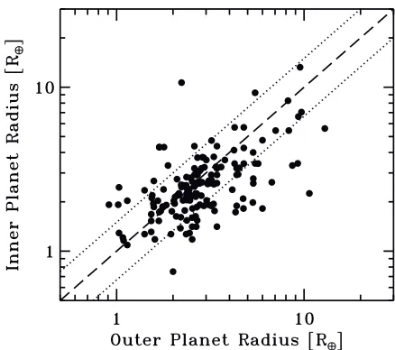
Figure 9.Comparison of the inner planet radius to the outer planet radius for each pair of planets, The dashed line delineates unity and the dotted lines mark the boundaries where one planet is 50% bigger than the planet to which it is compared (ratio=0.67 if the outer planet is larger and ratio=1.5 if the inner planet is larger).

Figure 10.Distribution of the planet radii for those planet pairs where one planet is>50% larger than the other planet. The top panel is for those planet pairs where the outer planet is larger than the inner planet (Rinner/Router0.67); the bottom panel is for those planet pairs where the inner planet is larger than the outer planet (Rinner/Router1.5).

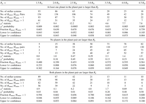
Figure 11.Fraction of planet pairs with (Rinner/Router<1) are plotted as a function of maximum planet radius. In the top panel, only those planet pairs are included that have at least one planet that is larger than a planet radiusRp. In the middle panel, only those planet pairs are included where both planets are smaller than a planet

radiusRp. In the bottom panel, only those planet pairs are included where both planets are larger than a planet radiusRp. The numbers underneath each data point list

the number of pairs in that bin. In each panel, the dashed-dot line and gray area delineate the fraction and uncertainties found for the entire sample (from Figure3); the dashed line delineates the 50% fraction.

distribution of the planet radii (Figure 8) and in the smaller median absolute deviations of the median planet radius for each stellar group (Table3).

This paper is not intended to provide a discussion of the occurrence rates of planets or a detailed analysis of the size distribution of planets (e.g., Howard et al.2012), but this may imply that the cooler (i.e., smaller) stars only produce smaller planets that do not preferentially follow a size hierarchy of planets. In fact, large planets around small stars may not form at all (Endl et al. 2003; Johnson et al. 2010) or, if they do, they may not survive their youth (e.g., van Eyken et al.2012). Thus, cool stars may only be left with a population of relatively small planets (Lopez et al.2012). The warmer stars, in contrast, appear to host a larger array of planet sizes with a slightly higher preference for the larger planets (>Neptune-sized) to be in longer orbits exterior to the orbits of the smaller planets. Given that there appears to be only a weak correlation with the planet-radii ratio and the orbital period (ratio), perhaps the formation and migration of large planets (perhaps in conjunction with photoevaporation of the innermost planets) is necessary for a radius hierarchy to be present.

3.3. Planet Radius

If hotter stars tend to show a planet radius hierarchy and the hotter stars also host relatively larger planets, then the planet hierarchy might be expected to be correlated with the planet size. In Figure9, we compare the sizes of the planet radii for the inner and outer planets for each pair of planets within the sample. The overall planet-radii ratio is near unity but there is more scatter below than above the unity line (i.e., smaller planets are interior to larger planets). There are 36 planet pairs where the outer planet is >50% larger than the inner planet (Rinner/Router 0.67); in contrast, there are only 13 planet pairs where the inner planet is >50% larger than the outer planet (Rinner/Router 1.5).

Table 4

Planet-radii Ratios Summary Group by Maximum Planet Radius

Rp= 1.5R_⊕ 2.0R_⊕ 2.5R_⊕ 3.0R_⊕ 3.5R_⊕ 4.0R_⊕ 4.5R_⊕

At least one planet in the planet pair is larger thanRp

No. of stellar systems 93 86 63 44 29 23 18

No. ofRinner/RouterPairs 154 138 106 74 49 42 29

No. ofRinner/Router<1 93 87 71 50 32 30 22

No. ofRinner/Router>1 61 51 35 24 17 12 7

χ2statistic 6.7 9.4 12.2 9.1 4.6 7.7 7.8

χ2probability 0.009 0.002 0.0005 0.003 0.03 0.005 0.005

FractionRinner/Router<1 0.603 0.630 0.670 0.676 0.653 0.714 0.759

Lower 1σconfidence 0.043 0.045 0.052 0.063 0.081 0.086 0.105

Upper 1σconfidence 0.041 0.043 0.048 0.058 0.073 0.075 0.084

No planets in the planet pair are larger thanRp

No. of stellar Systems 5 15 38 58 73 78 82

No. ofRinner/Routerpairs 5 20 53 85 110 117 130

No. ofRinner/Router<1 2 7 24 45 63 65 73

No. ofRinner/Router>1 3 13 29 40 47 52 57

χ2_{statistic 0.0 1.8 0.47 0.29 2.3 1.4 1.9}

χ2_{probability 1.0 0.18 0.49 0.59 0.13 0.23 0.16}

FractionRinner/Router<1 0.400 0.350 0.453 0.529 0.572 0.555 0.561

Lower 1σconfidence 0.253 0.088 0.076 0.060 0.052 0.050 0.048

Upper 1σconfidence 0.302 0.164 0.078 0.059 0.051 0.049 0.046

Both planets in the planet pair are larger thanRp

No. of stellar systems 89 67 42 21 13 11 10

No. ofRinner/Routerpairs 138 98 64 30 15 13 10

No. ofRinner/Router<1 82 59 42 21 10 8 6

No. ofRinner/Router>1 56 39 22 9 5 5 4

χ2statistic 4.9 4.1 6.2 4.8 1.7 0.69 0.4

χ2probability 0.03 0.04 0.01 0.03 0.20 0.40 0.50

FractionRinner/Router<1 0.594 0.602 0.656 0.700 0.667 0.615 0.600

Lower 1σconfidence 0.046 0.055 0.069 0.106 0.162 0.141 0.204

Upper 1σconfidence 0.044 0.053 0.064 0.091 0.135 0.172 0.180

planets are very small (e.g., Earth-sized<1.5R_⊕) planets. In contrast, for those planet pairs where the inner planet is much larger than the outer planet, the pairs are evenly split between relatively small outer planets (6/13 are<1.5R_⊕) and relatively large inner planets (5/13>4R_⊕).

It appears that for there to be a planet radius hierarchy, one of the planets most often needs to be∼Neptune-sized or larger. To explore this more closely, we have calculated the fraction of planet pairs with (Rinner/Router < 1), if at least one planet is larger than some maximum planet radius (Rp), or if both planets are smaller than that same maximum planet radius (Rp), or if both planets are larger than that same maximum planet radius. The fractions were calculated for maximum planet radii of Rp = [1.5,2.0,2.5,3.0,3.5,4.0,4.5]R⊕ (see Figure 11) and are tabulated in Table4.

If planet pairs with planets larger than 3R_⊕are excluded, the fraction is very near 50% with little preference for sequential planet ordering, but if one planet in the pair is larger than∼3R_⊕, the observed fraction of planet pairs withRinner/Router < 1 is 68±6%—a 3σseparation from the random ordering fraction of 50% (see Table4). Based upon theχ2_{statistic and probability} and the confidence intervals, the fraction of planet pairs is significantly above 50% only when Neptune-sized planets or larger are allowed in the pairs.

The fraction is most significant when Neptune-sized or larger planets are compared to planets of all sizes (top panel Figure11); the χ2 statistic are all >4 with a 1% probability that the non-50% fractions are achieved solely by chance. When the sizes of both planets are restricted to radii smaller than Neptune,

the fractions remain near or below 50% (middle panel Figure11 and Table4), with a15% probability of the observed fractions being generated by chance for the null-hypothesis distribution. When both planets within a planet pair are restricted to planets larger than a certain radius, sequential ordering of the planet sizes is still apparent, but is less significant (bottom panel Figure11and Table4). If both planets in a pair are3.0R_⊕, then the observed fraction of planet pairs where the inner planet is smaller than the outer planet is consistent with no planet size hierarchy. These results suggest that the size ordering primarily occurs when a system contains both super-sized (or Earth-sized) planetsandNeptune-sized or larger planets, and may be a direct result of the shepherding of smaller inner planets by larger outer planets (Raymond et al.2008).

4. SUMMARY

planet is smaller than the outer planet. If at least one planet in the planet pair is Neptune-sized or larger (3R_⊕), the fraction of inner planets being smaller than outer planets is≈68%±6%. However, if both planets are smaller than Neptune, then the fraction is consistent with random planet ordering (53%±6%) with no apparent size hierarchy.

The planet radius size hierarchy may be a natural conse-quence of planetary formation and evolution. In particular, the sequential ordering may be a result of a combination of core ac-cretion, migration, and evolution. Core accretion models predict that smaller planets are expected to form prior to and interior to the giant planets (Zhou et al.2005). Additionally, larger planets formed farther out may migrate inward, shepherding smaller planets inward as the planets move (Raymond et al.2008).

This scenario is consistent with the planet size hierarchy being observed for planet pairs involving Neptune-sized planets, but being absent for small planet pairs and for the planets around cool stars. For the cooler stars, the forming planets may begin migrating prior to starting rapid gas accretion (e.g., Ida & Lin 2005), coupled with a lower extreme ultraviolet luminosity that is not capable of substantially evaporating the planets (Lopez et al. 2012). For example, Lopez et al. (2012) suggest that the Kepler-11 planets did not form in situ, but rather, the planets formed beyond the snow line, migrated inward, and were evaporated by the star to their present sizes.

These scenarios (perhaps all in concert) predict a radius hierarchy of planets as a function of orbital distance from the central host star, in particular predicting that Neptune-sized and larger planets are outside super-Earth and terrestrial-sized planets. As Kepler discovers more planets in longer orbital periods, it will be interesting to learn if our solar system is indeed typical of the planetary architectures found in the Galaxy.

Kepler was competitively selected as the 10th NASA Dis-covery mission. The authors thank the many people who have madeKeplersuch a success. This paper includes data collected by theKeplermission; funding for theKeplermission is pro-vided by the NASA Science Mission directorate. This research has made use of the NASA Exoplanet Archive, which is oper-ated by the California Institute of Technology, under contract with the National Aeronautics and Space Administration un-der the Exoplanet Exploration Program. D.C.F. acknowledges

NASA support through Hubble Fellowship grant HF-51272.01-A, awarded by STScI, operated by AURA under contract NAS 5-26555. D.R.C. thanks the referee, theKeplerteam, Bill Borucki, Geoff Marcy, Stephen Kane, Peter Plavchan, Kaspar von Braun, Teresa Ciardi, and Jim Grubbs for very insightful and inspira-tional comments and discussions in the formation of this paper.

REFERENCES

Batalha, N. M., Borucki, W. J., Bryson, S. T., et al. 2011,ApJ,729, 27 Batalha, N. M., Rowe, J. F., Bryson, S. T., et al. 2012, arXiv:1202.5852 Borucki, W. J., Koch, D., Basri, G., et al. 2010,Sci,327, 977 Borucki, W. J., Koch, D. G., Basri, G., et al. 2011,ApJ,736, 19 Ciardi, D. R., von Braun, K., Bryden, G., et al. 2011,AJ,141, 108 Clopper, C. J., & Pearson, E. S. 1934,Biometrika, 26, 404

Endl, M., Cochran, W. D., Tull, R. G., & MacQueen, P. J. 2003,AJ,126, 3099 Fabrycky, D. C., Ford, E. B., Steffen, J. H., et al. 2012a,ApJ,750, 114 Fabrycky, D. C., Lissauer, J. J., Ragozzine, D., et al. 2012b, ApJ, submitted

(arXiv:1202.6328v2)

Fang, J., & Margot, J.-L. 2012,ApJ,761, 92

Fressin, F., Torres, G., Rowe, J. F., et al. 2012,Natur,482, 195

Gautier, T. N., III, Charbonneau, D., Rowe, J. F., et al. 2012,ApJ,749, 15 Howard, A. W., Marcy, G. W., Bryson, S. T., et al. 2012,ApJS,201, 15 Ida, S., & Lin, D. N. C. 2005,ApJ,626, 1045

Johnson, J. A., Aller, K. M., Howard, A. W., & Crepp, J. R. 2010,PASP, 122, 905

Latham, D. W., Rowe, J. F., Quinn, S. N., et al. 2011,ApJL,732, 24 Lissauer, J. J., Fabrycky, D. C., Ford, E. B., et al. 2011a,Natur,470, 53 Lissauer, J. J., Marcy, G. W., Rowe, J. F., et al. 2012,ApJ,750, 112 Lissauer, J. J., Ragozzine, D., Fabrycky, D. C., et al. 2011b,ApJS,197, 8 Lopez, E. D., Fortney, J. J., & Miller, N. K. 2012,ApJ,761, 59

Migaszewski, C., Slonina, M., & Gozdziewski, K. 2012,MNRAS,427, 770 Morton, T. D., & Johnson, J. A. 2011,ApJ,738, 170

Muirhead, P. S., Hamren, K., Schlawin, E., et al. 2012,ApJL,750, 37 Orosz, J. A., Welsh, W. F., Carter, J. A., et al. 2012,Sci,337, 1511

Press, W. H., Teukolsky, S. A., Vetterling, W. T., & Flannery, B. P. 2007, Numerical Recipes: The Art of Scientific Computing (3rd ed.; New York: Cambridge Univ. Press)

Raymond, S. N., Armitage, P. J., Moro-Mart´ın, A., et al. 2012,A&A,541, A11 Raymond, S. N., Barnes, R., & Mandell, A. M. 2008,MNRAS,384, 663 Santerne, A., D´ıaz, R. F., Moutou, C., et al. 2012,A&A,545, 76

Steffen, J. H., Fabrycky, D. C., Ford, E. B., et al. 2012a,MNRAS,421, 2342 Steffen, J. H., Ragozzine, D., Fabrycky, D. C., et al. 2012b,PNAS,109, 7982 Torres, G., Fressin, F., Batalha, N. M., et al. 2011,ApJ,727, 24

van Eyken, J. C., Ciardi, D. R., von Braun, K., et al. 2012,ApJ,755, 42 von Braun, K., Kane, S. R., & Ciardi, D. R. 2009,ApJ,702, 779

Walsh, K. J., Morbidelli, A., Raymond, S. N., O’Brien, D. P., & Mandell, A. M. 2011,Natur,475, 206