Factorised Contingency Planning
Bram Ridder
1, Michael Cashmore
2, Maria Fox
2, Derek Long
2, Daniele Magazzeni
2 Kings College London, London, WC2R 2LS[email protected],[email protected]
Abstract
In this paper we consider one of the hardest problems in plan-ning, contingency planning. Recent work has proposed trans-lations for a specific class of contingency planning problems, characterised asDeterministic POMDPs, to classical plan-ning problems. This class of contingency planplan-ning problems have deterministic actions and observations which makes it feasible to translate them into classical planning problems. This makes it possible to use mature classical planners like FF and Fast Downward to solve contingency planning problems. However, the translations proposed so far do not scale well and the results are not competitive with native contingency planners like POND and CLG. In this paper we improve upon previous translations by factorising the domain based on ex-ploiting mutually independent observation actions. We show that our approach scales better compared to previous offline approaches in domains that are factorisable. For domains that do not factorise well we show that our approach is on-par with previous offline approaches.
1
Introduction
Contingency planning deals with planning problems where the initial state is not fully known and the outcome of actions and observations are non-deterministic. This class of prob-lems is relevant to a wide range of real-life probprob-lems. For ex-ample, robotic systems have noisy sensors and the outcome of executing an action is uncertain to some degree. The re-cent interest in incorporating planning systems in robotic systems highlights the need for planning systems that can deal with uncertainty. Unfortunately, this class of problems is known as one of the hardest problems in planning (Rinta-nen 2004).
Early approaches encoded a contingent planning prob-lem as conjunctive, and disjunctive, normal formulae. For example, Contingent-FF (Hoffmann 2005), POND (Bryce, Kambhampati, and Smith 2006), or the related planners CNF and DNF (To, Pontelli, and Son 2011). One of the largest problems contingency planners face is that they do not scalevery well due to the representation of the belief state and the generation of the successor states.
In this paper we deal with arestrictedset of contingent planning problems that can be characterised asDeterministic
Copyright c2016, Association for the Advancement of Artificial Intelligence (www.aaai.org). All rights reserved.
POMDPs(Bonet 2009). Unlike general contingency plan-ning problems these problems have deterministic actions and observations. This restricted class of contingency plan-ning problems can effectively be translated into equivalent
classical planningproblems (Albore, Palacios, and Geffner 2009). The encoding of belief states is much easier as all the uncertainty is in the initial state and all observation actions are deterministic. Belief states can be encoded by tracking which possible initial states conform to the outcome of ob-servation actions. Successor states are generated by apply-ing actions to all these states.
Online planners like SDR (Brafman and Shani 2012b) and MPSR (Brafman and Shani 2012a) use translations to reduce the complexity of the original problem bysampling
a subset of all possible initial states and encoding the re-laxed problem as a classical planning problem. The found solution is used as a heuristic for action selection. CLG (Al-bore, Palacios, and Geffner 2009) maps contingent problems to non-deterministic problems, it translates the latter to a re-laxed problem that is solvable by a classical planner. The solutions of the relaxed problems are used an heuristic esti-mate. CLG can also be used as anoff lineplanner, where it finds a complete solution for all possible initial states.
K-Planner (Bonet and Geffner 2011) further restricts the set of contingency planning problems by imposing that vari-ables that are unknown in the initial state do not appear in the body of conditional effects. Contingent problems of this form are simple as they have a bounded contingent width of 1 (Bonet and Geffner 2014), so they can be translated into equivalent fully-observable non-deterministic planning problems that require no beliefs. Its translation is linear in the problem size for restricted contingent planning prob-lems. This translation only works if the state-space isfully connected, because the translation assumes that the planner can choose the outcome of observations. It creates a par-tial solution and if the actual observation does not match the chosen observation during execution a replan is triggered. Subsequent translations like (Palacios, Albore, and Geffner 2014) can findcomplete solutions to the restricted contin-gent planning problems and do not require the state-space to be fully connected.
modified FOND planner (PRP (Muise, McIlraith, and Beck 2012)) to solve it. Their planner and translation scales much better than the previous state-of-the-art planner CLG, albeit on a smaller class of problems. One additional benefit of PO-PRP is that it can detect strong cycles and produce very compact plans.
In this paper we explore the idea offactorisingthe con-tingency planning problem in order to reduce the space state and increase the scalability of contingency planners. The key idea is that the outcomes of all observations are not all dependent. E.g. in a logistics domain where a driver is un-sure about the location of his key for the truck and the lo-cation of a package he needs to pick up, it is clear that the location of the key and the whereabouts of the package are independent. In this paper we will explore how we can ploit these independence relationships and how we can ex-tract them from the planning problem.
Factorisation has been used in the context of belief track-ing for planntrack-ing problems with senstrack-ing. For example, Causal Belief Tracking (Bonet and Geffner 2014) decom-poses a problem into projected subproblems based on sets of variables that arecausally relevantto each other. Variables are causally relevant to each other if the uncertainty of one affects the uncertainty of the other. Causal Belief Tracking is an orthogonal approach, and trivial in the set of problems we consider. We use the same kind of decomposition in or-der to to speed up the planning process by factorising the original planning problem.
The rest of the paper is organised as follows. In Sec-tion 2 we formally define the contingency planning problem, in Section 3 we explore how we can detect independence relationships, in Section 4 we present our translation of a contingency planning problem by factorising the domain, in Section 5 we present the results of our novel translation and we conclude in Section 6 with a discussion and future work.
2
Contingency Planning
In this section we define the contingency planning problem. We use the PDDL (Ghallab et al. 1998) problem represen-tation used in Palacios et al. (Palacios, Albore, and Geffner 2014) (second translation).
Definition 1 — Problem Representation
A contingency planning problemP =hF, S0, AF, AO, Gi whereF is a set of atoms,S0 is the set of possible initial states, Gis a conjunction over F that represents the goal that needs to be achieved,AF is a set of actions that affect the world, andAOis the set ofsensingactions.
All the uncertainty is encoded in the initial belief stateS0. A belief state is maintained by tracking which factsf ∈F
are true for each states∈S0. We denote that a factfis true in statesasf /s.
Included inF is the proposition(active). This propo-sition describes whether the state concurs with the sensing actions made so far. Initially all initial statessareactive,
i.e. (active)/s,∀s∈S0. Xf denotes that a factf ∈F is
true in all active statesS⊆S0.
Every actiona∈AF∪AOhas a preconditionpre(a). An action is only applicable if its precondition is satisfied byall
active states. Every actiona ∈AF has a set of effects that are characterised bya:C →E, whereCis a formula that – when satisfied – adds the effectE.
An action af ∈ AO reveals the true value of the atom
f ∈ F. Whenever an observation actionaf is performed, the planning problem is split into two branches. One branch contains all the statesS> ⊂S0for whichf is true, the other branch contains the statesS⊥=S0\S>in whichf is false. The problem representation stores these branches in a
stack. Each time a sensing actionaf ∈ AO is applied, the states inS⊥are added to thestack, and these states are made inactive. When the goals are achieved in the active states the stack ispopped. This means that all states inS> are now made inactive and all states inS⊥– that were on the stack – are made active. A stack can be multiple levels deep. This happens when an observation is applied within a branch. The number of levels must be bounded when creating the model.
Included in F is the propositions (stack number) and
(level number), wherenumber is a symbol representing a number. These propostions are used to encode the stack.
(stack number)denotes that the state is stacked at the depth
number, while(level number)denotes the current size of the stack. Initially the stack is empty, soX(level 0).
For the full description of this translation, see Palacios et al. (Palacios, Albore, and Geffner 2014) (second transla-tion).
A plan for P is a branched plan: every time an obser-vation action is executed the plan branches contingently on the outcome of the observation. A solution to this planning problem requires a simple plan for all branches. Branched plans has been explored in the past, e.g. (Coles 2012) where the branches are contingent on the available resources dur-ing execution.
Example 1 Consider a problem where we are looking for our garage key and we know that it is in one of three boxes. Also we want to fix the flat tire of our car that is in the garage, but we do not know which of the four tires is flat. We can only access the garage by opening the door with the key.
Example 1 introduces an example problem we will use throughout the paper. There are 12 different states that we believe could be true, i.e. |S0| = 12. These are the Carte-sian product of the 3 possibilities for the key location and 4 possibilities for the flat tire. The solution to this problem is to find the key to the garage, open the door, then find the flat tire and fix it.
identical. In other words, the location of the key is indepen-dent of where we can expect to find the flat tire.
Definition 1 deals with this problem as if the locations of the key and the flat tire are correlated. For example, a branch might correspond to the key inbox 0andtire 3being flat, which is different from the case where we found the key inbox 1and andtire 3is flat. The solution requires a simple plan for each of the 12 branches.
3
Independence Relationships
In this section we define independence relationships be-tween observations actions. In Example 1, we are looking at two independent observations. Firstly we need to find a key, which is in three possible locations. After that we need to find and fix the flat tire of which there are four possible options, creating a possibility space of seven options.
Definition 2 — Independent Observations
Given a contingency planning problemhF, S0, AF, AO, Gi two observation actionsop, oq∈AOareindependentif and only if:
|Sp|/|S0|=|SpTSq|/|Sq|=|SpTS¬q|/|S¬q|
|Sq|/|S0|=|SqTSp|/|Sp|=|SqTS¬p|/|S¬p|
whereSα={s∈S0|α/s}.
We also observe transitive dependency relationships; for example, ifop is not independent ofoq andor is not inde-pendent ofoq thenopis not independent ofor.
Informally, two observations are independent if the come of either observation does not inform about the out-come of the other observation. For example, knowing the value ofqdoes not change the probability thatpis true.
Referring to Example 1:
|S(in key box0)|/|S0|
6
=
|S(in key box0)TS(in key box1)|/|S(in key box1)|
There are4total states in which the key is in box 0 out of the12states in total: (|S(in key box0)|/|S0|= 1/3). There are no states in which the key is in both box 0 and box 1: (|S(in key box0)
T
S(in key box0)|/|S(in key box1)|= 0). Hence, these observation actions that check if a key is in a box are not independent.
In contrast, knowing the location of the key does not in-form us about which tire is flat. For example:
|S(f lat tire0)|/|S0|
=
|S(f lat tire0)TS(in key box0)|/|S(in key box0)|
=
|S(f lat tire0)TS¬(in key box0)|/|S¬(in key box0)|
= 1/4
The observation actions to check the state of a tire are inde-pendent of those that observe whether a key is in a box.
We introduce the concept of a dependent observation set(DOS).
Definition 3 — Dependent Observation Set
Given a contingency planning problemhF, S0, AF, AO, Gi adependent observation setfor an observation actiona ∈ AOis defined as all observations actionsa0 ∈AO, such that
ais not independent ofa0.
In order to find the sets of observations that are dependent we compare all pairs of observation actions. Thus, finding the sets of observations that are dependent isO(|AO|2).
In Example 1 there are two DOSs: Dkey ={(find key box0),(find key box1),(find key box2)}andDtire={(check tire0),(check tire1),(check tire2),(check tire3)}.
4
Factorised Contingency Planning Problems
In this section we will discuss how we exploit the inde-pendence relationships between DOSs. Previous encodings of contingency planning problems into a classical planning problems make the implicit assumption that all observations are dependent. In this section we describe how we factorise the contingency problem such that observations that are part of oneDOS(e.g. finding the key) are independent from ob-servations that are part of anotherDOS(e.g. finding which tire is flat).4.1
Partial State Sets
The encoding in Definition 1 enumerates all the possible ini-tial states. However, such an encoding contains a lot of re-dundancies. Our encoding maps all possible initial states to partial state sets using the found DOSs, thereby reducing the number of states we need to encode.
Definition 4 — Partial State Set
Given the set of possible initial statesS0 and a DOSD ⊆
AO, we defineFD={f |of ∈D}as the set of all the facts that are observable by the observation actions inD. Given a states, a partial statesFD ⊆sis the value of the factsFD
ins. A partial state set is then defined asSD={sFD |s∈
S0}.
Informally, for every DOS (D) we map each possible ini-tial state to a parini-tial state that only contains the facts that can be observed by the observation actions inD. Note that a partial state set does not include duplicate partial states. There are two partial states sets in Example 1:
SDkey = {{(in key box0)},{(in key box1)},
{(in key box2)}}
SDtire= {{(f lat tire0)},{(f lat tire1)},
{(f lat tire2)},{(f lat tire3)}}
The partial states0 = Ts∈S0scontains those facts that are true across all possible initial states. The initial belief state can be represented as the Cartesian product ofs0and
SD, for each DOSD.
The number of partial state sets is usually much smaller than the original number of possible initial states. Returning to Example 1, we map the12possible initial states to8 par-tial states:s0,SDkey, andSDtire. In the worse case scenario
method fails gracefully as we fall back on a single partial state setS0.
4.2
Factorised Problem Representation
In our factorised problem representation the initial state is the partial state set{s0}, which is initiallyactive. The ob-servable facts are part of partial state sets.
For each pair of partial state setsSDandS0D, we define the actions: (access SD SD0)and(exit SD SD0), and the
facts:(accessedSD)and(parentSDSD0 ).
In order to observe facts in these partial state sets, the sets need to beaccessed. A partial state can only be accessed if and only if a single state is active. Accessing a partial state setSD0 from the accessed partial state setSD, makes
the current active state s ∈ SD inactive; updatesSD0 =
{s} ×SD0; and makesactivethe new set of states inSD0.
The partial state setSDbecomes theparentofSD0.
A partial state set can beexited. When weexit the ac-cessed partial state setSD0, we make each states ∈ SD0 inactive, andaccesstheparentpartial state setSDand make actives∈SD.SD0is no longeraccessed.
We use these new facts and actions in the construction of the Factorised Problem Representation, and describe them in detail below.
Definition 5 — Factorised Problem Representation GivenhF, S0, AF, AO, Gi, the set of partial state sets S, a factorised contingency planning problem is defined as
hF0, S0
0, A0F, AO, Giwhere:
• F0 = F ∪ S
SD∈S((accessed SD) ∪
S
SD0∈S (parent SDSD0))
• A0F = AF ∪ SSD,S
D0∈S((access SD SD0) ∪
(exit SDSD0))
• S0
0={s0}wheres0= (accessed S00)∪
T
s∈S0s
Definition 5 extends Definition 1 with theaccessandexit
actions, and associated facts.
The action(access SDSD0)has the precondition:
accessed(SD)
∧V
si,sj∈SD(¬(active si)∨ ¬(active sj))
and the effects:
¬accessed(SD)∧accessed(SD0)
V
s∈SD((active)/s→(parent SDSD0)/s)
V
s0∈S
D0(parent SDSD
0)/s
V
s∈SD¬(active)/s
V
s0∈S
D0(active)/s
0
V
s∈SD(f /s∧(active)/s)→(
V
s0∈S D0f /s
0), ∀f ∈F0
V
s∈SDf /s→ ¬f /s, ∀f ∈F
The precondition ensures that a new partial state set can only beaccessedif a single partial state is currentlyactive.
Upon accessing a partial state set, SD0, the new partial
state set becomesaccessedand the parentSDis no longer
accessed. The fact(parent SDSD0)is set true in all partial
states ofSD0 and in the singleactivestate ofSD.
All facts in which are true in the singleactivepartial state ofSD become true in all partial states ofSD0. Those facts
are made false in theactivestate ofSD.
Finally, the singleactivestate ofSDis set inactive, and all partial states ofSD0 become active.
Intuitively, the current knowledge is moved into the par-tial state set corresponding to one DOS. As in Definition 1, an observation actionaq can only be performed if the cur-rent belief state includes anactivestate in which the factqis false, and some state in whichqis true. Therefore, observa-tion acobserva-tions in the DOSD0can only be performed once the corresponding partial state setSD0has beenaccessedand its
partial states madeactive.
The action(exit SDSD0)has the precondition
accessed(SD0)∧(parent SDSD0)∧
V
s0∈S
D0¬∃n∈N(stack n)/s
0
and the effects:
accessed(SD)∧ ¬accessed(SD0)
V
s∈SDSSD0¬(parent SDSD0)/s
(parent SDSD0)/s→(active)/s ∀s∈SD
V
s0∈S
D0¬(active)/s
0
((parent SDSD0)/s
∧V
s0∈S D0f /s
0)→f /s ∀f ∈F0,∀s∈S D
(V
s0∈S D0f /s
0)→(V
s0∈S D0¬f /s
0) ∀f ∈F0
Intuitively, the exit action reverses the access action. Makingactivethe single partial statesthat was previously active in the parent partial state set. Moreover, when exiting a partial state setSD0, each fact which is true inallstates of
SD0is made true in the active partial states∈SD. We can
onlyexita partial state setSD0if and only if there is no state
s0 ∈SD0on the stack.
We use Example 1 to illustrate these actions. As estab-lished earlier, there are three partial state sets: S00, SDtire,
and SDkey. Initially only S
0
0 is accessed and s0 is ac-tive. The only fact that is true in all possible initial states is (door closed). Since the stack is empty, s0 =
{(door closed),(level0)}.
First we must find the key. In order to perform the obser-vations in DOSDkey, the partial state setSDkey must be ac-cessed. SDkey contains three partial states. Whenaccessed
we end up with the following belief state:
SDkey ={
{(in key box0),(active)}SF00,
{(in key box1),(active)}S
F00,
{(in key box2),(active)}SF00 }
where
F00={ (door closed),(accessed SDkey),
(parent S00SDkey),(level0)
}
In this belief state we can the perform the observation actions in Dkey. Performing the observationa(in key box0) yields the following belief state:
SDkey ={
{(in key box0),(active)}SF00,
{(in key box1),(stack0)}S
F00,
where
F00={ (door closed),(accessed SDkey),
(parent S00 SDkey),(level1)
}
The observation action puts on thestackall partial states that conflict with the observed fact,(in key box0). It makes these inactive. The remaining active state contains no un-certainty of the whereabouts of the key, so we can perform
(pickup key box0)to arrive at the belief state:
SDkey ={
{(holding key),(active)}SF00,
{(in key box1),(stack0)}S
F00,
{(in key box2),(stack0)}SF00 }
Subsequently we popthe stack, rendering the first state notactiveand other states active. Then, we perform the ob-servationandpickupactions in those states states as above. We end in the following belief state:
SDkey ={
{(holding key)}SF00,
{(holding key)}S
F00,
{(holding key),(active)}SF00 }
where
F00={ (door closed),(accessed SDkey),
(parent S00 SDkey),(level0)
}
The stack is empty, so we can nowexitthis partial state set. All facts that are true in each state in SDkey become
true in the parent partial state, s0. In our example, these facts are:(holding key),(door closed),and(level0)(we omit the facts(accessed SDkey)and(parent S
0
0SDkey)as
they are deleted by theexitaction). The current belief state becomes:
S00 ={ {(holding key),(door closed),(accessed S
0 0),
(level0),(active)} }
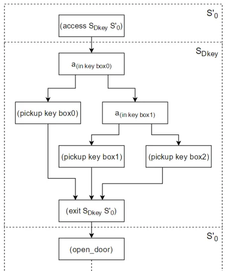
Figure 1 illustrates this process.
The door can be opened with the key. With the door open the flat tire can be found and fixed. Note that the branching tree built to pickup the key has collapsed into a single partial states0 ∈ S00. We know with certainty that, during execu-tion, we will have acquired the key. However, we do not knowhowthis key was acquired only that we have it. The remainder of the plan is therefore not contingent of where the key was found.
5
Results
In this section we present results obtained by using our fac-torisation method. Our baseline is the encoding described in Section 2. We allow 30 minutes per task and 2GiB of memory. We used FF-X (Hoffmann and Nebel 2001) solve both encodings. We expect our encoding toscalebetter at domains that are highly factorisable. Domains that cannot be factorised fail gracefully as we fall back on the previous encoding. We show results for the Contingent Benchmarks CLG Suite1.
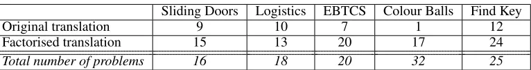
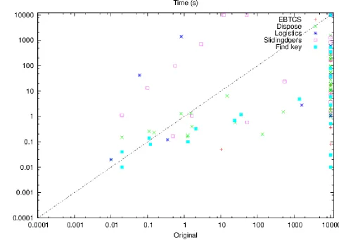
The results are depicted in Figure 2. The number of in-stances solved per domain are depicted in Table 1.
1
[image:5.612.325.551.53.323.2]http://www.ai.upf.edu/software/clg-contingent-planner
Figure 1: Solution to the example problem. The dashed box shows which partial state set is currentlyaccessed.
5.1
Sliding Doors
This domain models a set of corridors where an agent needs to move from the initial corridor to the goal corridor. Every corridor has a set of doors, one of which is open. The plan-ner needs to search for the open door in each corridor. The observation actions for every corridor are dependent, but ob-servation actions for different corridors are independent.
This domain is highly factorisable. In every corridor a single door is open and there are no dependencies between the doors in every corridor. Our encoding creates a partial state set for each corridor that encapsulates the knowledge about which door is open. We created 16 planning instances. The number of corridors ranges from 1 to 4 and the number of doors per corridor ranges from 2 to 5.
As the number of corridors grows, our factorised ap-proach outperforms the original encoding. Furthermore we manage to solve much larger and complex problem instances than the original encoding can deal with.
Sliding Doors Logistics EBTCS Colour Balls Find Key
Original translation 9 10 7 1 12
Factorised translation 15 13 20 17 24
[image:6.612.117.500.51.102.2]Total number of problems 16 18 20 32 25
Table 1: Number of problems solved per domain.
becomes too large to handle and our approach can solve in-stances the original encoding could not cope with.
One challenge in our encoding for this problem is theexit
action. Whenever we exit a partial state set, only those facts that are true in all active states are copied toS0. The planner needs to make sure that it only exits a partial state set when the location of the agent is equal in all active states. The higher the number of doors, the more states that the planner needs to manage per partial state set. However, as the num-ber of corridors increases we see that our approach scales better.
The number of actions in a plan cannot be compared di-rectly, as we have additional actions in our encoding (access
andexit). A plan for the original encoding is a complete tree where each traversal is a complete plan for one of the states. Whereas in our factorised encoding we have a more com-pressed plan as we force the planner to converge to a single state whenever we exit the partial state set. For problem in-stances that are not factorisable, we pay for the overhead and our plans are longer. However, for domains that factorise well, we find shorter plans in less time.
5.2
Logistics
The logistics domain models a number of cities which have a number of locations and an airport. Each city has a number of trucks that can move packages around in the city. For a package to reach another city it needs to be moved to an airport, and transported via an aeroplane to another city.
In this experiment we limit the domain to a single aero-plane and each city has a single airport and a single truck. The number of cities ranges from 1 to 2, the number of pack-ages ranges from 1 to 3, and the number of locations per city ranges from 1 to 3. Creating a total of 18 problem instances. Each package is hidden in a single city at one of its possi-ble locations. The planner needs to locate each package and deliver it to a destination in a different city. Packages can be located by trucks and aeroplanes, both trucks and aeroplanes can perform sensing actions to check if a package is at the same location the vehicle.
If there is only a single location per city, the problem is not a contingency problem as each packages can only be at a single location. In the original encoding this problem col-lapses in a single state, making it very easy to solve. How-ever, in our encoding each package is part of its ownpartial state setwhich makes the problem much harder to solve. For example, a problem instance where there are two cities, each consisting of a single locations, and three packages per city (six total) our encoding has seven partial state sets (one for each package in addition to the initial state), whilst the orig-inal encoding collapses the entire problem in a single state.
For problem instances with more locations, our encoding solves more problem instances and does it quicker. How-ever, we do not observe the improvement we expected. Whilst the problem is highly factorisable the planner strug-gles to exploits our encoding. Like the previous problem, the
exitandaccesspartial state sets seem to be the bottleneck. We will return to this discussion in our conclusions.
5.3
EBTCS
This domain encodes a bomb diffuse problem. To diffuse a bomb, we must find in which package it is hidden and subsequently flush it down the toilet.
In order to test whether our method scales better we have varied the number of bombs and the number of packages each bomb can be hidden in. The number of bombs ranges from 1 to 5 and the number of packages ranges from 2 to 5. For a total of 20 problem instances. We have limited the number of toilets in each problem instance to one.
Our method clearly scales better as the number of bombs and packages increase. In fact we manage to solve all the benchmark problems. The largest problem instance the pre-vious method manages to solve contains five bombs that can be hidden in two different packages. This problem instance has25 = 32possible initial states. In contrast, our method manages to solve the problem instance that has five bombs hidden in five packages which has55 = 3125possible ini-tial states. In our encoding, we encapsulate the whereabouts of each bomb in a partial state set, this results in5 partial state sets, each consisting of 5partial states. This reduces our encoding to25 + 1states.
5.4
Colour Balls
The colour balls domain is an interesting domain as there are two hidden facts per ball, its location and its colour. Both needs to be discovered before we can dispose the ball in the appropriate garbage container. In our encoding we have as many garbage containers as there are colours, each garbage container accepts one unique colour of balls. Furthermore, we made sure that all locations are fully connected.
The number of balls ranges from 2 to 3, the number of lo-cations ranges from 2 to 5, and the number of colours ranges from 2 to 5. In total there are 32 problem instances.
Figure 2: Scatterplot of the time it took (in seconds) to solve problem instances. Values of 10.000 denote instances that were not solved. We omitted results neither translation could find a solution to.
partial state sets per ball, one that encapsulates the colour a ball has and the other encapsulates the location of where the ball is plus one for the initial state.
5.5
Find Key
The final problem we explore is the find keyproblem that we have used as a rolling example througout the paper. The number of boxes and tires range from 1 to 5 for a total of 25 problem instances.
Given the set of keyskand the set of locationslthe num-ber of states that are created in the original encoding is equal to| l ||k|. In our encoding the number of partial states is equal to| l | +| k | +1. As the number of locations and keys increases our encoding to performs better as we have to deal with less partial states.
Our encoding solves all problem instances, except the problem instance with 5 keys and 5 tires.
6
Discussion and Future Work
In this paper we have presented a novel translation method that translates a contingency planning problem into a
clas-sical planning problem. Our method factorises the contin-gency planning problem by finding dependent observation sets, each set consists of actions whose observations are de-pendent. We presented an efficient algorithm to find these sets and presented how these sets are turned into partial state sets and how they are exploited in our translation.
Our translation is based on a previous encoding that enu-merates all possible states and encodes a stack mechanism in the planning domain to cope with uncertainty. The mapping we use to construct the partial state sets greatly reduces the number of states we need to encode for problem instances that are highly factorisable. For example, consider a prob-lem instance for thefind keydomain where we have five lo-cations and four keys. The previous method encodes 625 different states, whereas we only encode 21 partial states.
into a single state. Branches only occur in the context of a partial state set.
Our method manages to scale better and can solve larger problem instances faster. However, the encoding of a con-tingency planning domain into a classical planning problem is not flawless. We rely on the planner to find a branched plan in the context of partial state sets such that – when we exit that partial state set – all the facts that we require are identical for all states in the active states. That is why, as the number of states in a partial state set becomes too large, we struggle to find plans or take longer than the original ap-proach.
In future work we will explore the possibility of improv-ing performance by movimprov-ing the machinery that tackles the contingent nature of the problem inside the planner. We hy-pothesise that such a planner can find solutions faster, and al-low us to construct better heuristics. Whilst the RPG heuris-tic proved sufficient for the domains explored in this paper we want heursitics that are not agnostic to the contingent nature of the planning problem. For example, when FF cal-culates the heuristic values of successor states to the current state, it is unaware that inactive states on the stack have no influence on the current branch.
References
Albore, A.; Palacios, H.; and Geffner, H. 2009. A translation-based approach to contingent planning. InProc. of Int. Joint Conf. on Artificial Intelligence (IJCAI-09). Bonet, B., and Geffner, H. 2011. Planning under partial observability by classical replanning: Theory and experi-ments. InProceedings of the Twenty-Second international joint conference on Artificial Intelligence-Volume Volume Three, 1936–1941. AAAI Press.
Bonet, B., and Geffner, H. 2014. Belief tracking for plan-ning with sensing: Width, complexity and approximations.
J. Artif. Intell. Res. (JAIR)50:923–970.
Bonet, B. 2009. Deterministic pomdps revisited. In Pro-ceedings of the Twenty-Fifth Conference on Uncertainty in Artificial Intelligence, UAI ’09, 59–66. Arlington, Vir-ginia, United States: AUAI Press.
Brafman, R. I., and Shani, G. 2012a. A multi-path compila-tion approach to contingent planning. In Hoffmann, J., and Selman, B., eds., Proceedings of the Twenty-Sixth AAAI Conference on Artificial Intelligence, July 22-26, 2012, Toronto, Ontario, Canada. AAAI Press.
Brafman, R. I., and Shani, G. 2012b. Replanning in do-mains with partial information and sensing actions. Jour-nal of Artificial Intelligence Research45:565–600. Bryce, D.; Kambhampati, S.; and Smith, D. E. 2006. Plan-ning graph heuristics for belief space search. J. Artif. Int. Res.26(1):35–99.
Coles, A. J. 2012. Opportunistic branched plans to max-imise utility in the presence of resource uncertainty. In Pro-ceedings of the Twentieth European Conference on Artifi-cial Intelligence (ECAI-10).
Ghallab, M.; Isi, C. K.; Penberthy, S.; Smith, D. E.; Sun, Y.; and Weld, D. 1998. Pddl - the planning domain
def-inition language. Technical report, CVC TR-98-003/DCS TR-1165, Yale Center for Computational Vision and Con-trol.
Hoffmann, J., and Nebel, B. 2001. The FF planning sys-tem: Fast plan generation through heuristic search.Journal of Artificial Intelligence Research14:253–302.
Hoffmann, J. 2005. Contingent planning via heuristic for-ward search with implicit belief states. InIn Proceedings of ICAPS05, 71–80. AAAI.
Muise, C. J.; Belle, V.; and McIlraith, S. A. 2014. Comput-ing contComput-ingent plans via fully observable non-deterministic planning. In Brodley, C. E., and Stone, P., eds., Pro-ceedings of the Twenty-Eighth AAAI Conference on Arti-ficial Intelligence, July 27 -31, 2014, Qu´ebec City, Qu´ebec, Canada., 2322–2329. AAAI Press.
Muise, C. J.; McIlraith, S. A.; and Beck, J. C. 2012. Im-proved non-deterministic planning by exploiting state rel-evance. In McCluskey, L.; Williams, B.; Silva, J. R.; and Bonet, B., eds.,Proceedings of the Twenty-Second Interna-tional Conference on Automated Planning and Scheduling, ICAPS 2012, Atibaia, S˜ao Paulo, Brazil, June 25-19, 2012. AAAI.
Palacios, H.; Albore, A.; and Geffner, H. 2014. Compiling contingent planning into classical planning: New transla-tions and results. Models and Paradigms for Planning un-der Uncertainty: a Broad Perspective 65.
Rintanen, J. 2004. Complexity of planning with partial observability. InICAPS 2004. Proceedings of the Four-teenth International Conference on Automated Planning and Scheduling, 345–354. AAAI Press.