Improving the accuracy of general perturbations methods of spacecraft lifetime analysis

IAC-15-A6.4.6

IMPROVING THE ACCURACY OF GENERAL PERTURBATIONS METHODS FOR SPACECRAFT LIFETIME ANALYSIS

Emma Kerr

University of Strathclyde, Scotland, [email protected] Malcolm Macdonald

University of Strathclyde, Scotland, [email protected]

Using modern mathematic tool sets, various general perturbations methods such as the methods developed by the authors1,2, by Cook, King-Hele & Walker3 or by Griffin & French4 among others can be enhanced with the development of an average projected area model. A new method of determining the average projected area of a tumbling CubeSat is presented, which improves on the accuracy of the method recommended in Section 6.3 of the ISO standard 27852:2010(E)5. This enhancement can be applied to many different general perturbations methods and due to its simple mathematical nature it allows users to perform rapid Monte-Carlo analyses with thousands of permutations of the problem. Traditional numerical or even semi-analytical solutions would require a much greater length of time to produce an orbit lifetime prediction for a single permutation. For the range of CubeSat configurations presented it can be seen that the new method improves the error in the average projected area from, approximately 27% to within 5%. The enhancements are seen to outperform the ISO standard consistently and the ISO standard is seen to consistently overestimate the average projected area when considering non-cuboid spacecraft configurations, meaning that when applied to an orbit decay model it will consistently underestimate the orbit lifetime. However its worth lies not only in the improvement in accuracy but also in the time saved when considering space debris analysis or in initial mission design where many parameters may be unknown. In these situations the ability to swiftly provide solutions for thousands of permutations of the problem or to provide a range of predictions based on initial uncertainties and a confidence value for that range is invaluable. The enhanced solution has then been demonstrated using UKube-1 (COSPAR spacecraft identification 2014-037F) as a case study. It can be seen that the new method outperforms the ISO standard, with an error in the average projected area of 8.09% compared to the ISO standards 14.48%.

I. INTRODUCTION

Much attention has been given to developing general perturbations methods (often referred to as ‘analytical methods’) for orbit lifetime analysis and many methods exist, for example the various methods presented by King-Hele and co-authors based on power series expansions of eccentricity, semi-major axis and eccentric anomaly.3,6–12 The methods presented by Sharma using K-S elements offer another example.13–16 These methods focus variously on circular, low-eccentricity or high-eccentricity orbits, and deal with complications to the atmospheric friction (commonly referred to as ‘atmospheric drag’) calculation such as the oblateness of the atmosphere or the introduction of geopotential perturbations to the orbit propagation model. However, little focus has been given to improving the accuracy of these methods by refining the inputs such as the estimated cross-sectional area or the drag coefficient used in determining atmospheric drag.

Primary body atmospheric drag is the main contributor to artificial satellite orbit decay in Earth orbit below 1000 km altitude as it acts against the velocity vector resulting in a reduction in orbit semi-major axis. The magnitude of this frictional force is

directly proportional to the cross-sectional area of a spacecraft. This area is not always the area of a cross-section however, but instead is the area seen when observing the spacecraft along the velocity vector. When considering non-convex solids, for example a spacecraft with deployable panels, the area required for the atmospheric drag calculation is the area that would be orthographically projected onto a plane perpendicular to the velocity vector. Therefore herein this area will be referred to as the projected area.

Several methods of calculating the projected area have been presented; the method presented by Ben-Yaacov, Elderman and Gurfil provides the most promise for incorporation into general perturbations methods. It calculates the projected area by projecting each of the individual faces of a spacecraft onto a plane perpendicular to the required view vector then removing any shaded areas.17 This method provides a method for the estimation of the projected area of a spacecraft in fixed attitude relative to the velocity vector, however if the spacecraft tumbles this method would be incapable of determining an accurate projected area. In order to apply the projected area of a tumbling spacecraft to a general perturbations method a method to calculate the average projected area is required.

To the best of the authors knowledge the only method offering an average ‘cross-sectional area’ calculation for spacecraft is the ISO standard 27852:2010(E)5. This standard states that, in lieu of a more detailed numerical integration model, a flat plate model should be used. However this model is incapable of providing accurate results when considering any configuration other than a cuboid without deployable structures.

A correction factor for the ISO standard is introduced herein to model the average projected area of a CubeSat to a greater degree of accuracy. This method could, however, be extended to incorporate larger spacecraft. CubeSats offer an interesting test case however as they are becoming an increasing controversial topic in the space community. They are considered by some simply as debris due to their typically short orbit lifetimes and tendency to fail, while others dispute this classification.

II. AREA AVERAGING MODEL Calculating the expected average area of a tumbling spacecraft can be problematic as many factors can affect the mode of tumble. If the tumble is truly random, however, numerical methods can be used to simulate tumbling accurately and can be incorporated easily into special perturbations (numerical) methods for orbit propagation and orbit lifetime analysis. If, however, speed is to be considered general perturbations methods become more useful therefore to accurately simulate a tumbling spacecraft a method of calculating the average projected area of spacecraft during its orbit lifetime is particularly important.

Calculating the Average Projected Area

In order to assess the average projected area of a randomly tumbling spacecraft, it is assumed that the tumble is uniform and every aspect of the spacecraft will be seen equally often throughout the orbit lifetime. A uniform sphere of viewpoints is then set

up with the spacecraft at the centre and the projected area is calculated for each viewpoint using a method similar to that presented by Ben-Yaacov et al.17. The average of all of these values is then taken to be the average projected area.

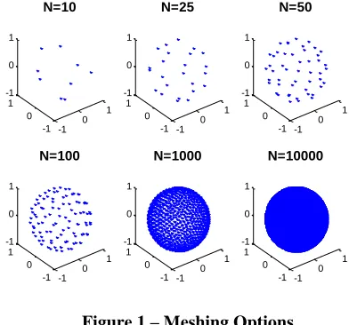
Six different spheres were considered, with increasing numbers of viewpoints, in order to make sure an accurate average is achieved. These spheres can be seen in Figure 1.

Figure 1 – Meshing Options

In order to compare accuracy a 3U CubeSat was used as a test case, the minimum area of this case will be the 10x10cm face. Using the 3U with 52 scenarios of various deployable panel sizes and positions as check for accuracy, the various spheres are compared; this comparison can be seen in Table 1.

Table 1 – Viewpoint Sphere Comparison

N Minimum

Area (m2₎

Average %Error in Projected Area

Standard Deviation in %Error in Projected Area

10 0.0250 1.021 0.715

25 0.0222 0.398 0.247

50 0.0201 0.172 0.148

100 0.0165 0.047 0.034

1000 0.0129 0.002 0.001

10000 0.0109 - -

From Table 1 it can be seen that the accuracy in the determining the minimum projected area is greatly improved by increasing the number of viewpoints used. However, it can also be seen that the average projected area is relatively unaffected by the number of viewpoints used. In fact the improvement in accuracy from 10000 down to 10 viewpoints is just over 1%. A comparison of the curve fit generated from this data can be seen in Figure 2. It should be noted that along the x-axis, in Figure 2, the ISO standard is plotted; this allows an easy comparison of the different configurations.

-1

0 1

-1 0 1 -1 0 1

N=10

-1

0 1

-1 0 1 -1 0 1

N=25

-1

0 1

-1 0 1 -1 0 1

N=50

-1 0 1

-1 0 1 -1 0 1

N=100

-1 0 1

-1 0 1 -1 0 1

N=1000

-1 0 1

-1 0 1 -1 0 1

Figure 2 – Comparison of Curve Fit

It can be seen in Figure 2 that the curve fit for the various spheres are extremely similar; therefore the 50-viewpoint sphere is used herein as it offers a compromise between the improvement in computational efficiency and the loss of accuracy. The following procedure could, however, be repeated using a greater number of viewpoints to improve the accuracy of the end result. This curve fit can now be used as a correction factor for the ISO standard. It should be noted, however, that it would only be applicable for the few configurations used to generate it, therefore it requires expansion to include further configurations before application.

The Correction Factor

The curve fit is expanded to include many CubeSat configurations in order to be a more effective correction factor for most probable configurations of CubeSats. These configurations vary from a basic 1U (i.e. 10cm cube) to 6U each with between 0 and 8 deployable panels set at various angles (90°, 135° & 180°). In this study 325696 unique configurations were considered, this encompasses the majority of configurations of CubeSats already in orbit; this is however an incomplete list. Larger CubeSats and larger deployable panels, than those considered herein, have been proposed, therefore if considering cases out with those considered herein the trend-line used should be adjusted to incorporate these possibilities.

To demonstrate the accuracy of the new correction factor it is compared to the average projected area calculation using the sphere of viewpoints and the ISO standard average cross-sectional area. Figure 3 shows the various configurations considered as different points. It can be seen that the average projected area calculated using the sphere of viewpoints is considerably smaller than the ISO standard area for the majority of configurations. There is one exception to this rule, however, for the few configurations where there are no deployable panels; in those cases the ISO standard is accurate.

Figure 3 – Comparison of Curve Fit and ISO Standard

It is apparent from Figure 3 that the curve fit generated using the new data set, including all probable CubeSat configurations, provides a more accurate estimate of the projected area than the ISO standard. Therefore this curve fit provided should be used as a correction factor to the ISO standard. The projected area of a CubeSat can therefore be calculated as

𝐴𝑃𝑟𝑜𝑗𝑒𝑐𝑡𝑒𝑑 = 0.7295 𝐴𝐼𝑆𝑂0.9624,

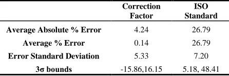
where AISO is the area determined using the ISO standard method. In order to properly quantify improvement the percentage error between the calculated value and the values provided by the correction factor and the ISO standard are compared in Figure 4 and Table 2.

Figure 4 – Accuracy Comparison of Correction Factor and ISO Standard

Table 2 – Accuracy Comparison of Correction Factor and ISO Standard

Correction Factor

ISO Standard

Average Absolute % Error 4.24 26.79

Average % Error 0.14 26.79

Error Standard Deviation 5.33 7.20

It can be seen clearly in both Figure 4 and Table 2 that the correction factor provides more accurate results than the ISO Standard. It can be seen from Table 2 that the average absolute error in the projected area calculated using the correction factor is much smaller than when using the ISO standard. It should be noted that the absolute error is used for this comparison as it provides a better understanding of the accuracy of the method, while the average error for the correction factor is approximately 0% the absolute error is 4.24%, meaning that on average error in the projected area is ±4.24%. It can also be seen in Table 2 that while the ISO standards 3rd standard deviation still excludes 0%, the correction factor is focussed around approximately 0%. The correction factor also produces a much smaller spread of errors as is demonstrated by the standard deviation. It can also be seen that the error in the ISO standard is consistently positive, meaning that the ISO standard always overestimates the area, excepting of course the no-deployable panel configurations. Though this may seem to give a conservative estimate of the projected area, it will give an orbit lifetime prediction that will be considerably shorter than could be expected. Therefore using the ISO standard to demonstrate space debris mitigation law compliance is not recommended. Given the data it is recommended, provided speed is not an issue, that the average projected area be calculated using the sphere of viewpoints. If, however, speed is to be considered the new correction factor should be used.

III. CASE STUDY – UKUBE-1

In order to show the effectiveness of the new correction factor, the method is demonstrated using the UKube-1 spacecraft (COSPAR spacecraft identification 2014-037F) as a case study. The new correction factor is applied to the general perturbations solution for low eccentricity orbit lifetime prediction developed by the authors.1,2 Conservatively it is assumed that the spacecraft is non-operational from the time it is launched, and hence its orbit must decay within 25 years of orbit insertion. Note that UKube-1 did operate following orbit insertion and hence this analysis is not a true-to-life prediction; such a prediction is not currently possible as the spacecraft is attitude controlled, however the prediction herein would have been applicable pre-launch for regulatory assessment purposes.

Using UKube-1’s actual launch date, specifications, and the relevant ISO standard5, as defined in Table 3, the average projected area can be calculated and the orbit lifetime can be predicted. Note the semi-major axis, eccentricity and inclination are taken from orbital tracking data, and as such are specified to the level of detail available.

Table 3 – UKube-1 Initial Orbit Parameters

Parameter Value

Beginning of Deorbit Phase (Assumed) 8th _{July 2014}

Total Mass at Launch 3.98 kg

Drag Coefficient (as specified by ISO

27852:2010(E)) 2.2

Initial Semi-Major Axis 7006.23 km

Initial Eccentricity 0.0003369

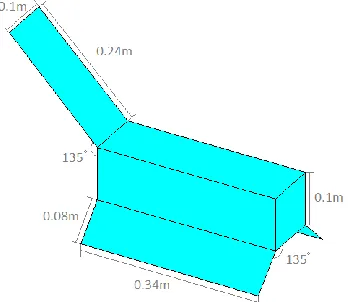
Initial Inclination 98.4032°

Given the geometry of UKube-1, as seen in Figure 5, the average area is calculated using the average projected area method with the viewpoint sphere, the correction factor and the ISO Standard method; the values calculated using of each of these methods are shown in Table 4.

Figure 5 - UKube-1 Geometry

Table 4 – Projected Area of UKube-1

Method Area (m2_{) % Error}

Average Projected Area 0.0683 -

Correction Factor Area 0.0628 -8.09

ISO Standard Area 0.0782 14.48

It can be seen that in this case the correction factor underestimates the projected area while the ISO standard method over estimates it. These areas are then applied to the orbit lifetime prediction and the orbit lifetime predictions attained can be seen in Table 5 and the projected decay can be seen in Figure 6.

Table 5 – Orbit Lifetime Prediction for UKube-1

Method Lifetime

(Years) % Error

Average Projected Area 12.2 -

Correction Factor Area 13.2 8.19

Figure 6 - Projected Decay of UKube-1

It can be seen in Table 5 that as expected the ISO standard method gives a shorter orbit lifetime than the projected area method. It can also be seen that the error in the orbit lifetime calculation has decreased for the ISO method and increased slightly for the curve fit, this is due to the complex nature of the relationship between orbit lifetime and projected area. Therefore it should be noted that the error cannot just be assumed to be the passed directly through; instead the standard deviation of the correction factor, as shown in Table 2, should be used to inform a Monte Carlo analysis of the orbit lifetime such as that shown in Figure 7.

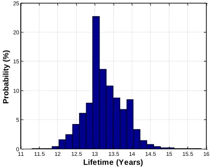
Figure 7 – Monte Carlo Analysis of UKube-1 Orbit Lifetime – Probability Distribution Showing

Effect of Variation in Projected Area

Figure 7 was generated by using a normal distribution, with the mean set as the average projected area calculated for UKube-1 using the correction factor with an error of approximately ±16% as indicted by the 3 sigma error in Table 2. The use of the 3 sigma bound means that approximately 99.7% of possible projected areas are captured; therefore there is a 99.7% probability that the actual orbit lifetime will also be captured. The predicted orbit lifetime range produced in this analysis was

11.3-15.9 years, with an average of 13.2 years; the orbit lifetime predicted using the sphere of viewpoints to calculate the average projected area was 12.2 years which falls within this range. Using the 2 sigma (approximately 95% of possible projected areas captured) bound this range becomes 12.0-14.9 years, which also includes the expected lifetime, 12.2 years. However the use of the more conservative 3 sigma interval is recommended, especially when considering regulatory compliance.

This method can also be used to provide an estimate of the maximum altitude that the spacecraft could have been launched to whilst still complying with best practise guidelines stating that a spacecraft should deorbit within 25 years of its end of life.18,19 The current solar cycle is considered a minimum cycle (specifically its maximum is low), however the magnitude of future cycles are unknown. Therefore conservatively the next two cycles are assumed to be minimum cycles to determine a maximum altitude as this will ensure that the spacecraft will de-orbit within the 25-year window. In the case of UKube-1 it can be seen from Figure 8 that the maximum allowable altitude would have been approximately 678km, 50km above the actual insertion altitude.

Figure 8 - UKube-1 predicted orbital lifetime versus initial altitude

IV. CONCLUSION

The ISO standard has been shown to consistently overestimate the average projected area when considering non-cuboid spacecraft configurations, i.e. CubeSats with deployable panels. This means that when applied to an orbit decay model it will consistently underestimate the orbit lifetime. However, it has also been shown that by the addition of a correction factor the ISO standard method can be used to produce a reliable estimate of the average projected area of a tumbling spacecraft. It is thereafter possible to incorporate the average projected area into general perturbations solutions using the newly introduced correction factor. Finally, using the

Time (years)

A

lt

it

u

d

e

(

k

m

)

0 2 4 6 8 10 12 14

0 100 200 300 400 500 600 700 800

0 1 2 3 4 x 10-4

E

c

c

e

n

tr

ic

it

y

Perigee Apogee Eccentricity

Lifetime (Years)

Probabil

ity

(%)

11 11.5 12 12.5 13 13.5 14 14.5 15 15.5 16 0

5 10 15 20 25

In

it

ia

l

A

lt

it

u

d

e

(

k

m

)

Predicted Lifetime (years)

0 5 10 15 20 25 30

0 100 200 300 400 500 600 700 800

correction factor it was found that the UKube-1 spacecraft was inserted into a lower orbit than necessary to comply with the 25-year limit set out by the ECSS and IADC guidelines.

V. ACKNOWLEDGEMENTS

Emma Kerr thanks the European Space Agency (ESA) for their support in attending this conference.

VI. REFERENCES 1 _{Kerr, E., and Macdonald, M., “A General}

Perturbations Method for Spacecraft Lifetime Analysis Incorporating Solar Activity,” In Draft

for Proceedings of the Royal Society A, 2015.

2 _{Kerr, E., and Macdonald, M., “A General} Perturbations Method For Spacecraft Lifetime Analysis,” 25th AAS/AIAA Space Flight

Mechanics Meeting, Wiliamsburg, VA, USA:

2015, pp. 1–15.

3 _{Cook, G. E., King-Hele, D. G., and Walker, D. M.} C., “The Contraction of Satellite Orbits under the influence of Air Drag I. With Sphericallly Symmetical Atmosphere,” Proceedings of the Royal Society A: Mathematical, Physical and

Engineering Sciences, vol. 257, 1960, pp. 224–

249.

4 _{Griffin, M. D., and French, J. R., Space Vehicle}

Design, Reston, VA: American Institute of

Aeronautics and Astronautics, Inc., 2004. 5 _{International Organisation for Standardisation,}

27852:2010(E): Space systems — Estimation of

orbit lifetime, 2010.

6 _{Cook, G. E., King-Hele, D. G., and Walker, D. M.} C., “The Contraction of Satellite Orbits Under the Influence of Air Drag II. With Oblate

Atmosphere,” Proceedings of the Royal Society A: Mathematical, Physical and Engineering

Sciences, vol. 264, 1961, pp. 88–121.

7 _{King-Hele, D. G., “The Contraction of Satellite} Orbits Under the Influence of Air Drag III. High-Eccentricity Orbits,” Proceedings of the Royal Society A: Mathematical, Physical and

Engineering Sciences, vol. 267, 1962, pp. 541–

557.

8 _{Cook, G. E., and King-Hele, D. G., “The} Contraction of Satellite Orbits Under the Influence of Air Drag IV. With scale height dependant on altitude,” Proceedings of the Royal Society A: Mathematical, Physical and

Engineering Sciences, vol. 275, 1963, pp. 357–

390.

9 _{Cook, G. E., and King-Hele, D. G., “The}

Contraction of Satellite Orbits under the Influence of Air Drag V. with Day-To-Night Variation in Air Density,” Philosophical Transactions of the

Royal Society of London A: Mathematical,

Physical and Engineering Sciences, vol. 259, Dec.

1965, pp. 33–67. 10

Cook, G. E., and King-Hele, D. G., “The Contraction of Satellite Orbits Under the Influence of Air Drag VI. Near-Circular Orbits with Day-to-Night Variation in Air Density,”

Proceedings of the Royal Society A: Mathematical, Physical and Engineering

Sciences, vol. 303, 1968, pp. 17–35.

11

King-Hele, D. G., and Walker, D. M. C., “The Contraction of Satellite Orbits under the Influence of Air Drag VII. Orbits of high eccentricity, with scale height dependent on altitude,” Proceedings of the Royal Society A: Mathematical, Physical

and Engineering Sciences, vol. 411, 1987, pp. 1–

17.

12 _{King-Hele, D. G., and Walker, D. M. C., “The} Contraction of Satellite Orbits Under the Influence of Air Drag VIII. Orbital lifetime in an oblate atmosphere, when perigee distance is perturbed by odd zonal harmonics in the

geopotential,” Proceedings of the Royal Society A: Mathematical, Physical and Engineering

Sciences, vol. 414, 1987, pp. 271–295.

13 _{Sharma, R. K., “A third-order theory for the effect} of drag on Earth satellite orbits,” Proceedings of the Royal Society A: Mathematical, Physical and

Engineering Sciences, vol. 438, 1992, pp. 467–

475.

14 _{Sharma, R. K., “Analytical approach using KS} elements to near-Earth orbit predictions including drag,” Proceedings of the Royal Society A: Mathematical, Physical and Engineering

Sciences, vol. 433, 1991, pp. 121–130.

15 _{Sharma, R. K., “Contraction of high eccentricity} satellite orbits using K-S elements with air drag,”

Proceedings of the Royal Society A: Mathematical, Physical and Engineering

Sciences, vol. 454, 1998, pp. 1681–1689.

16 _{Sharma, R. K., “Contraction of satellite orbits} using KS elements in an oblate diurnally varying atmosphere,” Proceedings of the Royal Society A: Mathematical, Physical and Engineering

Sciences, vol. 453, Nov. 1997, pp. 2353–2368.

17 _{Ben-Yaacov, O., Edlerman, E., and Gurfil, P.,} “Analytical technique for satellite projected cross-sectional area calculation,” Advances in Space

Research, vol. 56, Jul. 2015, pp. 205–217.

18 _{ECSS Requirements & Standards Devision, Space}

Product Assurance: Safety 3.1.9, Noordwijk:

1996.

19 _{Inter-Agency Space Debris Coordination} Committee, “IADC-02-01 Space Debris