MeyerChapter2013

(1)

CHAPTER 1 INFORMATION-THEORETIC GENE

SELECTION IN EXPRESSION DATA

PATRICK E. MEYER AND GIANLUCA BONTEMPI

MACHINE LEARNING GROUP, COMPUTER SCIENCE DEPARTMENT,

UNIVERSIT ´E LIBRE DE BRUXELLES, BELGIUM.

{PMEYER,GBONTE}@ULB.AC.BE

1.1 INTRODUCTION

Genome-wide patterns of gene expression represent a snapshot of the state of a cell in a given condition. Using different snapshots, taken under different conditions, it becomes possible to build statistical models that can efficiently classify and predict new snapshots. A typical application of such techniques consists in discovering new molecular signatures of tumor cells for diagnostic and prognostic purposes [52, 53]. However, the detection of functional relationships between genes as well as the design of effective models from expression data is a major statistical challenge, mainly because of the data dimensionality. Expression datasets are typically characterized by a low number of noisy samples together with a high number of variables. As a result, even a simple predictive model such as a linear regression cannot be used without eliminating irrelevant and redundant variables as a first step [30]. A number of experimental studies [28, 6, 46] have shown that the elimination of irrelevant and redundant variables as well as the selection of synergetic variables [35, 24] can dramatically increase the predictive accuracy of models built from data. Moreover, variable selection can decrease future measurements and storage requirements [20] while increasing the intelligibility of a model.

Please enter\offprintinfo{(Title, Edition)}{(Author)} at the beginning of your document.

(4)

In order to derive efficient methods of variable selection, formal definitions of relevance, redundancy andsynergy of variables have been defined. Information theory, a theory introduced for data transmission and signal compression [48] and widely used in areas such as statistics, physics, economics or biology, provides a particularly adapted framework for measuring, quantifying and defining variable interactions [38].

The outline of this chapter is the following. Section 1.2 introduces the curse of dimensionality. Section 1.3 focuses on widely used variable exploration strategies. Section 1.4 intoduces the information-theoretic framework. Section 1.5 recalls vari-able selection techniques which have been proposed in the literature. Section 1.6 introduces estimation techniques that can be used for implementing the selection strategies on the basis of observed data.

1.2 THE CURSE OF DIMENSIONALITY

A natural question arises when it comes to make experiments or measurements: “how many experiments do I need in order to obtain a clear signal in my data?” or even “how many genes can I select when I have made 100 experiments”?

(5)

VARIABLE SELECTION EXPLORATION STRATEGIES 3

1.3 VARIABLE SELECTION EXPLORATION STRATEGIES

Let us consider the following problem: givenda number of variables to select, is there an algorithm that can select the optimal subset of variables of a given size?

Unfortunately, various results, like the theorem by Cover and Van Campenhout [14], show that finding the optimal subset of sizedamongnvariables requires to test

all

n d

combinations of subsets. However, this is impossible in practice, since

it would take too much time to compute all of them. Hence, search heuristics have been used to reach a good predictive subset of variables.

Let us denoteAthe search space of

n d

subsets of random variables ofX

having sized. Variable selection can be seen as a combinatorial optimization problem [28] which depends on:

1. a method of exploring the spaceA(including the starting point and the stop criterion),

2. an evaluation function returning a measure of accuracy.

More formally the problem is: givenninput variablesXand a performance measure F :A→R, find the subsetXS ⊂Xwhich maximizes the performance,

X_Smax= arg max

XS∈A

F(XS) (1.1)

Exploration strategies can be classified into three main categories of combinatorial optimization algorithms namely optimal search, stochastic search and sequential search(see [21], chapter 4).

1. Optimal search strategies include exhaustive search and branch-and-bound methods [21]. Their high computational complexity makes them impracticable with a high number of inputs and, for this reason, they are not discussed in this work.

2. Stochastic search strategies are also calledrandomized or non-deterministic [45] because two runs of these methods (with the same inputs) will not neces-sarily lead to the same result [16]. These methods explore a smaller portion of the search spaceAby using rules often inspired by nature. Some examples are: simulated annealing [16], tabu search [16] and genetic algorithms [55, 16].

(6)

Because of their simplicity and their wide adoption in the variable selection com-munity, we focus here on the three main sequential strategies namely the forward selection, the backward one and the bi-directional one.

In the following, we denote byX the complete initial set of variables and by XM ET H

i ∈ X, i ∈ A = {1,2, ..., n} the variable selected at each step by the method M ET H. XS and XR are the set of selected variables and the set of remaining variables respectively. Hence, at each stepX = {XS, XR}. Xi orXj usually denotes a variable inXRor inXS, respectively.

1.3.1 Forward Selection search

Forward Selection [9, 28] is a sequential search method that starts with an empty set of variables,XS =φ. At each step, it selects the variableXtthat brings the best improvement (in terms of a given evaluation criterionF(·). A pseudo-code of the method is given in Algorithm 1.1. As a consequence of the sequential process, each selected variable influences the evaluations of the following steps.

This search has been widely used in variable selection, (see [9, 6, 28]). The forward selection algorithm selects a subset ofd < nvariables indsteps and explores only

Pd₋1

i=0(n−i)subsets.

However, this search has some weaknesses:

1. two variables that are synergetic (i.e., highly relevant only once taken together, see 1.4.3) appear as not relevant if taken individually and are as consequence ignored by this procedure,

2. selecting the best variable at each step does not mean selecting the best subset. Indeed, suppose that we have the following situation:

Y =f(X5, X4, X3) +N(0, σ1) =f(X1, X2) +N(0, σ2) (1.2)

whereN(µ, σ)denotes a normally distributed noise with meanµand variance σ. If we have, the following order of univariate relevance:

rel(X5)> rel(X1)> rel(X2)> rel(X4)≥rel(X3) (1.3)

and

σ1> σ2 (1.4)

the best subset should beX1,2={X1, X2}because the variance of the noise

is smaller. Also, there are less variables in the latter combination, which usually lead to a lower number of parameters to estimate in a model. How-ever, the forward selection algorithm will, in many cases, select the subset X3,4,5 = {X5, X4, X3}. Indeed, it first selects X5 becauseX5is the most

relevant variable. GivenX5, the best improvement can be brought byX4, and

(7)

VARIABLE SELECTION EXPLORATION STRATEGIES 5

Algorithm 1.1

Inputs: input variables X, the output variable Y, a maximal subset size d >0,a performance measure F(·) to maximize

XS:=φ XR:=X

while (|XS| < d) maxscore:=−∞

for all the inputs Xi in the search space XR

Evaluate F(XS,i) for the variable Xi with XS the subset of selected variables.

if ( F(XS,i)> maxscore) Xt:=Xi

maxscore:=F(XS,i) end-if

end-for XS:=XS,t XR:=XR₋t end-while

Output: the subset XS

1.3.2 Backward Elimination search

Backward elimination [9, 28, 39] is a search method that starts by evaluating a subset containing all the variablesXS = X and progressively discards the least relevant variables. For instance, at the second step, the method comparesnsubsets ofn−1

inputs. The variableXtassociated with the least favorable improvement of accuracy is eliminated. The process is repeated until it yields the chosen number of inputsd (see Algorithm 1.2). This method does not suffer from the risk of ignoring a pair of complementary variables as it is the case for forward selection.

Algorithm 1.2

Inputs: input variables X (the input space), the output variable Y, a minimal subset size d >0, and a performance measure F(·) to maximize

XS:=X

while (|XS| > d) worstscore:=∞

for all inputs Xj in the subset XS

Evaluate F(XS₋j), with all inputs of the subset XS without Xj

if ( F(XS₋j)<worstscore) Xt:=Xi

worstscore:=F(XS₋j) end-if

end-for XS:=XS₋t end-while

(8)

1.3.3 Bi-directional search

The strengths of the forward selection and of the backward elimination can be combined in different manners.

As an example, let 26 random variables constitute the search space and be denoted by letters of the alphabet. Let the best subset of four variables be denoted by the letters{B, E, S, T}. The forward and the backward approaches can be combined in different ways:

• by using a backward elimination on a subset selected with a forward search [9].

If a forward selection has selected the subset{C, B, E, S, T, D, F, G}, then, we can use a backward elimination in order to keep the most important variables of the subset, and reach the subset{B, E, S, T}.

• by performing a stepwise approach [39, 9]: At each step, choose the best action between eliminating a variable or selecting one.

In our example, we may at some stage have selected the subset{E, A, S, T}. The stepwise algorithm chooses between adding a variable that brings the best improvement{B, E, A, S, T}or eliminating the less important variable

{E, S, T}.

• by using sequential replacement [39, 9]: This procedure consists in replacing k≥1variables at each step.

In our example, we can imagine at some stage having the subset{P, E, S, T} that becomes the subset{B, E, S, T}after an iteration. The pseudo-code of the algorithm fork= 1is described in Algorithm 1.3.

Algorithm 1.3

Inputs: a selected subset of inputs XS,the set of remaining

variables XR, the output variable Y,and a performance measure

F(·) to maximize

do

for all inputs Xi in the remaining variables XR

Evaluate F(XS,i) end-for

Xt1:= arg maxXiF(XS,i)

for all for all inputs Xj in the subset XS

Evaluate the F(XS₋j) end-for

Xt2:= arg maxXjF(XS−j)

(9)

RELEVANCE, REDUNDANCY AND SYNERGY 7

end-do while Xt16=Xt2

Output: the subset XS

1.4 RELEVANCE, REDUNDANCY AND SYNERGY

In order to improve the resolution of the two variable selection problems stated above, i.e., subset estimation and search of good combination, many variable selection criteria have been developped in the past decade. These criteria focus on 1) select relevant variables without having to estimate accurately the full joint distribution of a subset 2) guide the heuristic search in the space of combinations.

These variable selection criteria have been built around three main notions: rele-vance, redundancy and synergy. These three notions can be efficiently formulated in an information-theoretic framework that is introduced in the following subsections. For simplicity, we consider here discrete variables though the theory can be extended to the continuous variable case.

1.4.1 Relevance

In this section entropy, conditional entropy and mutual information are defined. These notions will be intensively used in the following in order to define relevance, redundancy and synergy.

Theentropy[10] of a discrete random variableY with probability mass function p(Y)is defined by:

H(Y) =H(p(Y)) =−X

y∈Y

p(y) logp(y) =EY

log 1

p(y)

(1.5)

Note that this definition remains valid for a discrete random vector (i.e. a subset of random variables).

The usual unit of the entropy is thebit. However, other units are sometimes chosen for this measure. The unit depends on the base taken for the logarithm of Eq 1.5, base 2 for bit, base 10 forban. Thedeciban(one tenth of a ban) is also known as a useful measure of belief since 10 decibans correspond to an odds ratio of 10:1; 20 decibans to 100:1 odds, 30 decibans to 1000:1, etc [25]. The natural logarithm (base e) is increasingly used for computational reasons and in this case the unit is thenat.

Theconditional entropyofY givenXis,

H(Y|X) =H(Y, X)−H(X) (1.6)

This quantity measures the uncertainty of a variable once another one is known. The reduction of entropy due to conditioning can be quantified by a symmetric measure calledmutual information[10]:

(10)

Themutual informationbetweenXandY is,

I(Y;X) =X

x∈X

X

y∈Y

p(x, y) log

p(x, y) p(x)p(y)

(1.8)

Mutual information can be also viewed as a divergence between the joint distri-butionp(X, Y)and the product distributionp(X)p(Y)[10] or between the marginal distributionp(X)and a conditional distributionp(X|Y). As a consequence, when two variables are independent, their mutual information is null and the higher the dependency between the variables, the higher the value of the mutual information. When the two variables are identical, this measure reaches its maximum and is equal to the entropy of the variable, i.e.,I(X;X) =H(X).

The mutual information is a natural measure of relevance since it quantifies the dependency level between random variables. The use of mutual information as relevance measure traces back to [11]. Later, [50] introduced a selection criterion called theinformation bottleneckwhich uses also mutual information as a relevance measure. [29] defines the relevanceof a setXSto an output variableY as the mutual informationI(XS;Y).

As a result, the relevance of an input variableXiknowing a setXS to an output variableY is the gain of relevance resulting from usingXiadditionally toXS:

I(Xi;Y|XS) =I({XS, Xi};Y)−I(XS;Y) (1.9)

This quantity is precisely the conditional mutual information [10]. Its normalized version (i.e. constrained to range between zero and one) has been introduced by [5] in a variable selection procedure.

Note that it is possible to increase the information of a variable with another by appropriate conditioning, as shown in the following example.

LetY andX be two independent random variables andZ be a random variable defined as a deterministic function ofY andX(see Eq. 1.10).

X →Z←Y (1.10)

AsXandY are independent, we haveI(X;Y) = 0and sinceZ=f(X, Y), we obtainI(X;Y|Z)>0. As a result, the conditional mutual information is higher than the mutual information, i.e. I(X;Y|Z)> I(X;Y), which means that conditioning can increase relevance.

1.4.2 Redundancy

(11)

RELEVANCE, REDUNDANCY AND SYNERGY 9

betweennsets of random variablesX1, X2, ..., Xnis,

R(Xi;...;Xn) = n

X

i=1

H(Xi)−H(X1, X2, ..., Xn) (1.11)

Note that in the two-variables case,

R(Xi;Xj) =H(Xi) +H(Xj)−H(Xi, Xj) =I(Xi;Xj) (1.12)

While the relevance measure concerns the relation between inputs and outputs, the bivariate redundancy measure applies exclusively to input variables.

1.4.3 Synergy

Synergy and redundancy are two sides of a coin that has been calledvariable in-teraction.The definition of variable interaction in information-theoretic terms can be found in the seminal paper of [34] and, more recently, in [23].

The interaction amongnsets of random variables,X1, X2, ..., Xnis defined as:

C(X1;X2;...;Xn) = n

X

k=1

X

S⊆{1,...,n}:|S|=k

(−1)k+1H(XS) (1.13)

Given a random vectorX and a random variable Y the link between mutual informationI(X;Y)and interaction information is made explicit by the following formula from [29].

I(X;Y) =P_i_∈_AC(Xi;Y)−

P

i,j∈AC(Xi;Xj;Y)

+...+ (−1)n+1_C₍_X

1;X2;...;Xn;Y)

(1.14)

withC(Xi;Y) =I(Xi;Y).

In plain words, mutual information can be seen as a series where higher order terms are corrective terms that represent the effect of the multivariate interaction. In most cases, the measure of interaction is positive and it indicates that thensets of variables share a common information (redundancy). However, interaction can be negative. In the latter case, the variables are said to be complementary [35] or synergetic [2].

The synergy effect was mentioned in several variable selection papers [28, 20, 23, 24] and has been explicitely used in variable selection algorithms only recently [29, 35, 59].

In particular, the synergy between two random featuresXiandXjand the output

Y (n= 3)

−C(Xi;Xj;Y) =−H(Xi)−H(Xj)−H(Y)

+H(Xi, Xj) +H(Xi, Y) +H(Xj, Y)−H(Xi, Xj, Y)

=I(Xi,j;Y)−(I(Xi;Y) +I(Xj;Y))

(1.15)

(12)

indeed, that the joint information of two random variables, i.e.,I(Xi,j;Y)can be higher than the sum of their individual informationI(Xi;Y)andI(Xj;Y).

An example of synergy is Example 1.4.1 where conditioning increase relevance. Another known illustration of this phenomenon is the XOR problem as pointed out by [28]:

X1 X2 Y =X1⊕X2

1 1 0

1 0 1

0 1 1

0 0 0

One can see thatX1andX2have a null relevance individually, i.e. I(X1;Y) = 0,

I(X2;Y) = 0, whereas togetherX1,2has a maximal relevance, i.e. I(X1,2;Y) =

H(Y)>0. Synergy explains why a combination of apparently irrelevant variables can perform efficiently in a learning task. It also gives an intuition behind the Cover and Van Campenhout theorem [14] mentionned earlier, that requires to test all combinations of subset to find the optimal one.

1.5 INFORMATION-THEORETIC FILTERS

Variable selection methods based on mutual information are also called information-theoretic filters.

Let us start by stating the objective of aninformation-theoretic filter:

Given a training datasetDmofmsamples, an output variableY,ninput variables

Xand an integerd≤n, find the subsetXS⊆Xof sizedthat maximizes the mutual

informationI(XS;Y).

In other words, the objective offilters variable selection(for a givend), is to find the subsetXS, with|XS|=d, such that:

X_Smax= arg max

XS⊆X:|XS|=d

I(XS;Y) (1.16)

(13)

INFORMATION-THEORETIC FILTERS 11

In the following, we review the most important filter selection methods found in the literature which are based on information theory. We present the algorithms by stressing when and where the notion of relevance, redundancy and synergy are used.

1.5.1 Variable Ranking

This methodvariable ranking(RANK) returns a ranking of variables on the basis of their individual mutual informations with the output. This means that, givenninput variables, the method first computesntimes the quantityI(Xi, Y),i = 1, . . . , n, then ranks the variables according to this quantity and eventually discards the least relevant ones [17, 3].

The main advantage of this method is its low computational cost. Indeed, it requires onlyncomputations of bivariate mutual information. The main drawback derives from the fact that possible redundancies between variables are not taken into account. Indeed, two redundant variables, yet highly relevant taken individually, will be both well-ranked. On the contrary, two variables could be synergetic to the output (i.e., highly relevant together) while being poorly relevant once each taken individually. As a consequence, these variables could be badly ranked, or even eliminated, by a ranking filter.

1.5.2 Fast Correlation Based Filter

Fast Correlation Based Filter(FCBF) is a ranking method combined with a redun-dancy analysis which has been proposed in [58]. The FCBF starts by selecting the variable (in the remaining variablesXR) with the highest mutual information, denoted byX_iF CBF. Then, all the variables which are less relevant toY than redun-dant toX_iF CBF are eliminated from the list. For example,Xiis removed from the remaining variable setXRif

I(Xi;XiF CBF)> I(Xi;Y)

At the next step, the algorithm repeats the selection and the elimination steps. The procedure stops when no more variable remains to be taken into consideration.

In other words, at each step, the set of selected variablesXSis updated with the variable

X_iF CBF = arg max

Xi∈XR

I(Xi;Y) (1.17)

and the set of remaining variablesXRis updated by removing the set

{Xi ∈XR−i : I(Xi;Y)< I(Xi;XiF CBF)} (1.18)

This method is affordable because a few (less thann2_{) evaluations of bivariate}

(14)

Note that in [58], a normalized measure of mutual information called thesymmetrical uncertaintyis used, i.e. SU(X, Y) = _H₍2_XI(₎₊X;_HY₍)_Y₎. This measure helps to improve the performances of the selection by penalizing inputs with large entropies.

1.5.3 Backward elimination and Relevance Criterion

LetX_Smax⊂Xbe the target subset, i.e., the subsetXS of sized, that achieves the maximal mutual information with the output (1.16). By the chain rule for mutual information [10],

I(X;Y) =I(X_Smax;Y) +I(X_Rmax;Y|X_Smax) (1.19)

whereXR=X−S is the set difference between the original set of inputsXand the set of variablesXSselected so far.

The backward elimination (using mutual information) [47] starts withXS =X and, at each step, eliminates from the set of selected variableXS, the variableXjback having the lowest relevance onY,

X_jback= arg min

Xj∈XS

I(Xj;Y|XS−j) (1.20)

In other words,Xback

j is an approximation ofXRmaxin (1.19). The approximation is exact for a subset sized=n−1of one variable less than the complete set. The elimination process is then repeated until the desired size is reached. However, this approach is intractable for large variable sets since the beginning of the procedure requires the estimation of a multivariate density that includes the whole set of variables X.

1.5.4 Markov Blanket Elimination

The Markov blanket elimination [30] consists in approximatingI(Xj;Y|XS−j)in (1.20) byI(Xj;Y|XMj)withXMj ⊂XS−j a subset of variables, i.e. the Markov

blanket, having limited fixed sizek. The algorithm proceeds in two phases. First, for every variableXj in the selected setXS,kvariablesXMj are selected among

the variablesXS−j. Second, the least relevant variableXjM B (conditioned on the selected subsetXMj ⊆XS−j) is eliminated, i.e.,XS =XS\X

M B j .

X_jM B= arg min

Xj∈XS

I(Xj;Y|XMj) (1.21)

The process is repeated until the selected variable setXS contains no more ir-relevant and redundant variables, or when the desired subset size is reached. The method is named from the fact thatXMj is an approximate Markov blanket. In

[30], the Pearson’s correlation coefficient [26] is used in order to find thekvariables most correlated to the candidateXj. Thesekvariables are considered as the Markov blanketXMj of the candidateXj. In this way, only linear dependencies between

(15)

very slow. In fact, finding a Markov blanket is itself a variable selection task. As a result, this method is adapted to large dimensionality problems only with very strong assumptions on the structure ofXM.

1.5.5 Forward Selection and Relevance Criterion

A way to sequentially maximize therelevance(REL) quantityI(XS;Y)in (1.16), is provided by the chain rule for mutual information [10]:

I(XS0;Y) =I(XS;Y) +I(Xi;Y|XS) (1.22)

whereXS0 =XS,iis the updated set of variables. Rather than maximizing the left-hand side term directly, the idea of the forward selection combined with the relevance criterion consists in maximizing sequentially the second term of the right-hand term, I(Xi;Y|XS). In other words, the approach consists in updating a set of selected variablesXSwith the variableXiRELfeaturing the maximum relevance.

In analytical terms, the variableXREL

i returned by the relevance criterion at each step is,

X_iREL= arg max

Xi∈XR

{I(Xi;Y|XS)} (1.23)

whereXR=X₋Sis the difference between the original set of inputsXand the set of variablesXS selected so far. This strategy prevents from selecting a variable which, though relevant toY, is redundant with respect to a previously selected one. This algorithm has been used in [5, 3, 7, 47]. In [5], a normalized version of relevance is used.

Although this method is appealing, it presents some major drawbacks. The estimation of the relevance requires the estimation of large multivariate densities. For instance, at thed-th step of the forward search, the search algorithm requiresn−d evaluations, where each evaluation requires in turn the computation of a(d+ 1) -variate density. It is known that for a larged, the estimations are poorly accurate and/or computationally expensive [44]. In particular in the small sample settings (around one hundred), having an accurate estimation of large (d >3) multivariate densities is difficult (see 1.2). For these reasons, the recent filter literature adopt selection criteria based on bi- and trivariate densities at most.

1.5.6 Forward Selection and Conditional Mutual Information Maximization criterion

TheConditional Mutual Information Maximization criterion(CMIM) approach [18] proposes to select the variableXi ∈ XR whose minimal relevance I(Xi;Y|Xj) conditioned to each selected variable taken separatelyXj ∈XS, is maximal. This requires the computation of the mutual information ofXi and the outputY, condi-tioned on each variableXj∈XSpreviously selected.

(16)

X_iCM IM = arg max

Xi∈XR { min

Xj∈XS

I(Xi;Y|Xj)} (1.24)

A variableXican be selected only if its information to the outputY has not been caught by an already selected variableXj.

The CMIM criterion is an approximation of the relevance criterion,

X_iREL= arg max

Xi∈XR

{I(Xi;Y|XS)}

whereI(Xi;Y|XS)is replaced byminXj∈XS(I(Xi;Y|Xj)).

[18] shows experiments where CMIM is competitive with FCBF [58] in selecting binary variables for a pattern recognition task. This criterion selects relevant vari-ables, avoids redundancy, avoids estimating high dimensional multivariate densities and does not ignore complementarity two-by-two. However, it does not necessar-ily select a variable complementary to the already selected variables. Indeed, a variable that has a high negative interaction to the already selected variable will be characterized by a large conditional mutual information with that variable but not necessarily by a large minimal conditional information. In the XOR problem, for instance, the synergetic variables have a null relevance taken alone. In that case,

minXj∈XSI(Xi;Y|Xj) = 0and CMIM would not select those variable.

1.5.7 Forward Selection and Minimum Redundancy - Maximum Relevance criterion

TheMinimum Redundancy-Maximum Relevance (mRMR) criterion has been pro-posed in [44, 51, 43] in combination with a forward selection search strategy. Given a setXS of selected variables, the method updatesXS with the variableXi ∈XR that maximizesvi−zi, whereviis a relevance term andzi is a redundancy term. More precisely,viis the relevance ofXito the outputY alone, andziis the average redundancy ofXito each selected variablesXj ∈XS.

vi=I(Xi;Y) (1.25)

zi=

1 |XS|

X

Xj∈XS

I(Xi;Xj) (1.26)

X_iM RM R= arg max

Xi∈XR

{vi−zi} (1.27)

(17)

A justification of MRMR given by the authors [44] is that

I(X;Y) =H(X) +H(Y)−H(X, Y) (1.28)

with

R(X1;X2;...;Xn) = n

X

i=1

H(Xi)−H(X) (1.29)

and

R(X1;X2;...;Xn;Y) = n

X

i=1

H(Xi) +H(Y)−H(X, Y) (1.30)

hence

I(X;Y) =R(X1;X2;...;Xn;Y)−R(X1;X2;...;Xn) (1.31)

where,

• the minimum of the second termR(X1;X2;...;Xn)is reached for independent variables since, in that case, H(X) =P_iH(Xi)andR(X1;X2;...;Xn) =

P

iH(Xi)−H(X) = 0. Hence, if a subset of variables XS is already selected, a variableXishould have a minimal redundancyI(Xi;XS)with the subset. Pairwise independency does not guarantee independency. However, the authors approximateI(Xi;XS)with_|_S1_|

P

j∈SI(Xi;Xj).

• the maximum of the first termR(X1;X2;...;Xn;Y)is attained for maximally dependent variables.

Qualitatively, in a sequential setting where a selected subsetXSis given, indepen-dence between the variables inXis reached by minimizing 1

|XS| P

Xj∈XSI(Xi;Xj)' I(Xi;XS)and maximizing dependency between the variables ofX and ofY, i.e., by maximizingI(Xi;Y).

Although the method addresses the issue of bivariate redundancy through the term zi, it does not capture synergy between variables. This can be ineffective in situations like Example 1.4.1 where, although the set{X, Z}is very relevant for predictingY, onceXhas been selectedZwill not since

1. the redundancy termziis large due to the redundancy ofX andZ,

2. the relevance termviis small sinceZalone is not relevant toY.

(18)

1.5.8 Forward Selection and Minimum Interaction - Maximum Relevance criterion

TheMinimum Interaction-Maximum Relevance(mIMR) criterion, also calledDouble Input Symmetrical Relevance(DISR) in a previous version, has been proposed in [35, 8] in combination with a forward selection search strategy. Given a setXS of selected variables, the method updatesXSwith the variableXi∈XRthat maximizes

vi−wi, whereviis a relevance term andwiis an interaction term. As in mRMR,vi is the relevance ofXito the outputY alone, however in mIMR the second termwi is an average interaction ofXito each selected variablesXj∈XS.

vi=I(Xi;Y) (1.32)

wi=

1 |XS|

X

Xj∈XS

C(Xi;Xj;Y) (1.33)

XimIM R = arg max Xi∈XR

{vi−wi} (1.34)

At each step, this method selects the variable which has the best trade-off between relevance and interaction. At step d of the forward search, the search algorithm computes n−d evaluations where each evaluation requires the estimation of a bivariate density plusdtrivariate ones. Assuming normally distributed variables, trivariate densities can even be computed with bivariate terms, leading to much faster selection of variables. This criterion eliminates redundant variable (because they are penalized by a positivewi) but also tends to select synergetic variable (because of their negativewi) while avoiding the estimation of multivariate densities.

A theoretical justification of mIMR given by the authors is that

I(XS;Y)≥

1

d 2

X

Xi∈XS X

Xj∈XS

I(Xi,j;Y) (1.35)

with

arg max

Xi∈XS X

Xj∈XS

I(Xi,j;Y) = arg max Xi∈XS

 

I(Xi;Y)−

1 |XS|

X

Xj∈XS

C(Xi;Xj;Y)

  

(1.36)

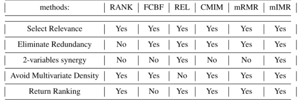
1.5.9 A theoretical comparison of filters

The presented criteria can be analyzed under different perspectives. We stress in Table 1.1,

(19)

FAST MUTUAL INFORMATION ESTIMATION 17

2. the ability of a criterion to avoid the estimation of large multivariate densities and

3. whether it returns a ranking of variables.

Table 1.2 reports a comparative analysis of the different techniques in terms of computational complexity of the evaluation step.

methods: RANK FCBF REL CMIM mRMR mIMR

Select Relevance Yes Yes Yes Yes Yes Yes

Eliminate Redundancy No Yes Yes Yes Yes Yes

2-variables synergy No No Yes No No Yes

Avoid Multivariate Density Yes Yes No Yes Yes Yes

Return Ranking Yes No Yes Yes Yes Yes

Table 1.1 Comparison of the properties (relevance, redundancy and synergy, ability to avoid estimation of large multivariate densities, ability to rank the variables) that are taken into account in each selection criterion.

variable evaluation: RANK REL CMIM mRMR mIMR

calls of mutual information 1 1 d d+ 1 d+ 1

k-variate density 2 d+ 1 3 2 3

computational cost O(C) O(d×C) O(d×C) O(d×C) O(d×C)

Table 1.2 The computational cost of a variable evaluation using rel, cmim, mrmr, mimr withCbeing the cost of a mutual information estimation.

We observe from Tables 1.2 and 1.1 that the mIMR criterion avoids redundant variables, multivariate density estimation, but selects synergetic variables (up to the second order), at the same computational cost than CMIM and mRMR. Numerous ex-perimental studies have shown the performances of mRMR and mIMR on expression datasets [38, 8].

1.6 FAST MUTUAL INFORMATION ESTIMATION

(20)

between computational load and accuracy in a variable selection purposes [38, 41]. However, it should be noted that most filters exposed above could be used with other estimators or even with other evaluation functions/ similarity measures than mutual information.

Mutual information computation requires the determination of three entropy terms (see Section 1.4.1):

I(X;Y) =H(X) +H(Y)−H(X, Y)

An effective entropy estimation is then essential for computing mutual information. Entropy estimation has gained much interests over the last decade[13] and most approaches focus on reducing the bias inherent to entropy estimation.

For microarray datasets, bias reduction should not be the only criterion to choose an estimator. Bias reduction should be traded with speed/computational complexity of the estimator. Indeed, in variable selection and network inference, mutual information estimation routines are expected to be called a huge number of times and used for estimating tasks with the same number of variables and the same amount of samples. Since filters consists mainly in comparing information-theoretic quantities, the correct ranking of the estimated quantities is much more important than the correct estimation of the quantities. A similar conclusion has been reached in [33, 41]. We refer the reader to [42, 13, 4, 40, 12] for alternative approaches of entropy and mutual information estimation.

1.6.1 Discretizing variables and empirical estimation

We describe here the equal frequency discretization since it has been reported in [57] Meyer as one of the most efficient discretization method.

The equal frequency discretization scheme consists in partitioning the interval

[a, b]into|Xi|intervals, each having the same number,m/|Xi|, of data points [15, 56, 32]. As a result, the intervals can have different sizes. If the|Xi|intervals have equal frequency, then the computation of entropy is straightforward:log_|X1

i|.

The value of the number of bins|Xi|controls a trade-off. With a too high|Xi|, each bin will contain a few number of points, hence the variance is increased, whereas a too low|Xi|will introduce a too high loss of information [10]. A classical choice of|Xi|is given by the samples square root

√

m[56]. One justification given for that choice is that the ratiom/|Xi| becomesm/

√

m = √m, hence there are as many bins as the average number of points per bin. Note also, that when estimating the entropy of a bivariate distribution where each variable has√mbins, the number of bins of the joint distribution is upper-bounded by|Xi| ≤ √m×√m = m. As a result, the empirical entropy estimator should not be too biased when combined with this choice of|Xi|.

(21)

FAST MUTUAL INFORMATION ESTIMATION 19

ˆ

Hemp(X) =−X

x∈X

#(x) m log

#(x)

m (1.37)

where#(x)is the number of data points having valuex. Because of the convexity of the logarithmic function, underestimates ofp(x)cause errors onE[_log1_p₍_x₎]that are larger than errors due to overestimations. As a result, entropy estimators are biased downwards, that is,

EHˆemp(X)≤H(X). (1.38)

It has been shown in [42] that

1. the variance of the empirical estimator is upper-bounded by a term

(logm)2

m

which depends only on the number of samples

2. the asymptotic bias is−|X |−₂_m1and depends on the number of bins|X |[42]. As

|X | m, this estimator can still have a low variance but the bias can become very large [42].

The computation ofHˆemp₍_X₎_{has an}_O₍_m₎_{complexity cost.}

The Miller-Madow correction is given by the following formula which is the empirical entropy corrected for the asymptotic bias,

ˆ

Hmm(X) = ˆHemp(X) +|X | −1

2m (1.39)

where|X |is the number of bins with non-zero probability. This correction, while adding no computational cost, reduces the bias without changing variance. As a result, the Miller-Madow estimator is often preferred to the naive empirical entropy estimator.

1.6.2 Assuming Normally Distributed Variables

Another way to deal with continuous variables without discretizing variables and decreasing the computational cost, is to assume that variables follow a well known probability distribution, such as the Gaussian one.

LetX be a multivariate Gaussian, having a density function,

f(X) = p 1

(2π)n_|_V_|exp

(−1 2(x−µ)

T_V−1₍_x₋_µ₎₎

(1.40)

with meanµand covariance matrixV.

The (differential) entropy of this distribution is [10]

H(X) = 1

2ln{(2πe)

n_|_V_|} _(1.41)

(22)

As a result, the mutual information between two normal distributions is given by [22]

I(Xi, Xj) =

1 2log

σiiσjj

|V|

(1.42)

whereσiiandσjj are the standard deviations ofXiandXjrespectively. Hence

I(Xi, Xj) =−

1

2log(1−ρ

2₎ _(1.43)

with ρ being the Pearson’s correlation [26] between Xi and Xj. Note that the complexity of estimatingρˆ2_is_O₍_m₎_{, whith}_m_{is the number of samples.}

1.7 CONCLUSIONS

Variable selection algorithms are mostly composed of two parts: a search strategy and an evaluation function. In the case of information-theoretic filters a third component is given by the mutual information estimator. In this chapter we have introduced eight different information-theoretic evaluation functions together with three heuris-tics searches and two mutual information estimators. The three sequential heurisheuris-tics searches introduced, namely the forward, the backward and the bi-directional selec-tion, share with the two mutual information estimators, the empirical and the gaussian, a low computational cost coupled with a growing literature of good empirical results. Having a low computational cost is critical in large datasets such as microarray data where the number of subset combinations is very high. An additional requirement brought by typical expression datasets is the ability to deal with a low number of samples. Most of the selection criteria presented here use combinations of only bi-and trivariate probability distributions in order to reduce the effect of the curse of dimensionality. Indeed, the latter require exponentially more samples for estimating larger joint distribution. Finally we a have introduced the notion of relevance, redun-dancy and synergy out of an information-theoretic framework in order to understand and compare each method’s ability to combine those bi- and trivariate distributions in an efficient setting.

REFERENCES

1. H. Almuallim and T. G. Dietterich. Learning with many irrelevant features. In Proceed-ings of the Ninth National Conference on Artificial Intelligence (AAAI91), pages 547–552. AAAI Press, 1991.

2. Dimitris Anastassiou. Computational analysis of the synergy among multiple interacting genes.Molecular Systems Biology, 2007.

3. R. Battiti. Using mutual information for selecting features in supervised neural net learning. InIEEE Transactions on Neural Networks, 1994.

(23)

REFERENCES 21

5. D. A. Bell and H. Wang. A formalism for relevance and its application in feature subset selection.Machine Learning, 41(2):175–195, 2000.

6. A. Blum and P. Langley. Selection of relevant features and examples in machine learning. Artificial Intelligence, 97:245–271, 1997.

7. B. V. Bonnlander and A. S. Weigend. Selecting input variables using mutual informa-tion and nonparametric density estimainforma-tion. In Proceedings of the 1994 International Symposium on Artificial Neural Networks (ISANN94), 1994.

8. G. Bontempi and P. E. Meyer. Causal filter selection in microarray data. InInternational Conference On Machine Learning (ICML), 2010.

9. R. Caruana and D. Freitag. Greedy attribute selection. InInternational Conference on Machine Learning, pages 28–36, 1994.

10. T. M. Cover and J. A. Thomas.Elements of Information Theory. John Wiley, New York, 1990.

11. R. T. Cox.Algebra of Probable Inference. Oxford University Press, 1961.

12. G. Darbellay and I. Vajda. Estimation of the information by an adaptive partitioning of the observation space.IEEE Transactions on Information Theory, 1999.

13. C. O. Daub, R. Steuer, J. Selbig, and S. Kloska. Estimating mutual information using b-spline functions - an improved similarity measure for analysing gene expression data. BMC Bioinformatics, 5, 2004.

14. L. Devroye, L. Gy¨orfi, and G. Lugosi. A Probabilistic Theory of Pattern Recognition. Springer-Verlag, 1996.

15. J. Dougherty, R. Kohavi, and M. Sahami. Supervised and unsupervised discretization of continuous features. InInternational Conference on Machine Learning, pages 194–202, 1995.

16. J. Dreo, A. Petrowski, P. Siarry, and E. Taillard. M´etaheuristiques pour l’Optimisation Difficile. Eyrolles, 2003.

17. W. Duch, T. Winiarski, J. Biesiada, and A. Kachel. Feature selection and ranking filters. InInternational Conference on Artificial Neural Networks (ICANN) and International Conference on Neural Information Processing (ICONIP), pages 251–254, June 2003.

18. F. Fleuret. Fast binary feature selection with conditional mutual information.Journal of Machine Learning Research, 5:1531–1555, 2004.

19. D. Franc¸ois, F. Rossi, V. Wertz, and M. Verleysen. Resampling methods for parameter-free and robust feature selection with mutual information. Neurocomputing, 70(7-9):1276– 1288, 2007.

20. I. Guyon and A. Elisseeff. An introduction to variable and feature selection. Journal of Machine Learning Research, 3:1157–1182, 2003.

21. Isabelle Guyon, Steve Gunn, Masoud Nikravesh, and Lotfi A. Zadeh.Feature Extraction: Foundations and Applications. Springer-Verlag New York, Inc., 2006.

22. S. Haykin.Neural Networks: A Comprehensive Foundation. Prentice Hall International, 1999.

23. A. Jakulin and I. Bratko. Quantifying and visualizing attribute interactions, 2003.

(24)

25. E. T. Jaynes. Probability Theory: The Logic of Science. Cambridge University Press, 2003.

26. M. G. Kendall, A. Stuart, and J. K. Ord.Kendall’s advanced theory of statistics. Oxford University Press, Inc., 1987.

27. M. B. Kennel, J. B. Shlens, H. D. I. Abarbanel, and E. J. Chichilnisky. Estimating entropy rates with bayesian confidence intervals.Neural Computation, 17(7), 2005.

28. R. Kohavi and G. H. John. Wrappers for feature subset selection. Artificial Intelligence, 97(1-2):273–324, 1997.

29. I. Kojadinovic. Relevance measures for subset variable selection in regression problems based on k-additive mutual information.Computational Statistics and Data Analysis, 49, 2005.

30. D. Koller and M. Sahami. Toward optimal feature selection. InInternational Conference on Machine Learning, pages 284–292, 1996.

31. I. Kononenko. Estimating attributes: Analysis and extensions of RELIEF. InEuropean Conference on Machine Learning, pages 171–182, 1994.

32. H. Liu, F. Hussain, C. Lim Tan, and M. Dash. Discretization: An enabling technique. Data Mining and Knowledge Discovery, 6, 2002.

33. A. A. Margolin, I. Nemenman, K. Basso, C. Wiggins, G. Stolovitzky, R. Dalla Favera, and A. Califano. ARACNE: an algorithm for the reconstruction of gene regulatory networks in a mammalian cellular context. BMC Bioinformatics, 7, 2006.

34. W. J. McGill. Multivariate information transmission.Psychometrika, 19, 1954.

35. P. E. Meyer and G. Bontempi. On the use of variable complementarity for feature selection in cancer classification. In F. Rothlauf et al., editor,Applications of Evolutionary Computing: EvoWorkshops, volume 3907 ofLecture Notes in Computer Science, pages 91–102. Springer, 2006.

36. P. E. Meyer, K. Kontos, F. Lafitte, and G. Bontempi. Information-theoretic inference of large transcriptional regulatory networks. EURASIP Journal on Bioinformatics and Systems Biology, Special Issue on Information-Theoretic Methods for Bioinformatics, 2007.

37. P. E. Meyer, D. Marbach, S. Roy, and M. Kellis. Information-theoretic inference of gene networks using backward elimination. InInternational Conference on Bioinformatics and Computational Biology (Biocomp), 2010.

38. P. E. Meyer, C. Schretter, and G. Bontempi. Information-theoretic feature selection using variable complementarity. IEEE Journal of Special Topics in Signal Processing, 2(3), 2008.

39. A.J. Miller.Subset Selection in Regression Second Edition. Chapman and Hall, 2002.

40. I. Nemenman, W. Bialek, and R. de Ruyter van Steveninck. Entropy and information in neural spike trains: Progress on the sampling problem. Physical Review Letters, 69, 2004.

41. C. Olsen, P. E. Meyer, and G. Bontempi. On the impact of entropy estimation on transcriptional regulatory network inference based on mutual information. EURASIP Journal on Bioinformatics and Systems Biology, 2009.

(25)

REFERENCES 23

43. H. Peng and F. Long. An efficient max-dependency algorithm for gene selection. In36th Symposium on the Interface: Computational Biology and Bioinformatics, may 2004.

44. H. Peng, F. Long, and C. Ding. Feature selection based on mutual information: criteria of max-dependency, max-relevance, and min-redundancy.IEEE Transactions on Pattern Analysis and Machine Intelligence, 27(8):1226–1238, 2005.

45. L. Portinale and L. Saitta. Feature selection.Applied Intelligence, 9(3):217–230, 1998. 46. G. Provan and M. Singh. Learning bayesian networks using feature selection. Inin Fifth

International Workshop on Artificial Intelligence and Statistics, pages 450–456, 1995.

47. F. Rossi, A. Lendasse, D. Franc¸ois, V. Wertz, and M. Verleysen. Mutual information for the selection of relevant variables in spectrometric nonlinear modelling. Chemometrics and Intelligent Laboratory Systems, 2:215–226, 2006.

48. C. E. Shannon. A mathematical theory of communication.Bell System Technical Journal, 1948.

49. M. Studen´y and J. Vejnarov´a. The multiinformation function as a tool for measuring stochastic dependence. InProceedings of the NATO Advanced Study Institute on Learning in graphical models, pages 261–297, 1998.

50. N. Tishby, F. Pereira, and W. Bialek. The information bottleneck method. InProceedings of the 37-th Annual Allerton Conference on Communication, Control and Computing, 1999.

51. G. D. Tourassi, E. D. Frederick, M. K. Markey, and Jr. C. E. Floyd. Application of the mutual information criterion for feature selection in computer-aided diagnosis. Medical Physics, 28(12):2394–2402, 2001.

52. M. J. van de Vijver, Y. D. He, L. J. van’t Veer, H. Dai, A. A. Hart, D. W. Voskuil, G. J. Schreiber, J. L. Peterse, C. Roberts, M. J. Marton, M. Parrish, D. Atsma, A. Witteveen, A. Glas, L. Delahaye, T. van der Velde T, H. Bartelink H, S. Rodenhuis, E. T. Rutgers, S. H. Friend, and R. Bernards. A gene-expression signature as a predictor of survival in breast cancer.New England Journal of Medecine, 347, 2002.

53. L. J. van ’t Veer, H. Dai, M. J. van de Vijver, Y. D. He, A. A. Hart, M. Mao, H. L. Peterse, K. van der Kooy, M. J. Marton, A. T. Witteveen, G. J. Schreiber, R. M. Kerkhoven, C. Roberts, P. S. Linsley, R. Bernards, and S. H. Friend. Gene expression profiling predicts clinical outcome of breast cancer.Nature, 406, 2002.

54. W. Wienholt and B. Sendhoff. How to determine the redundancy of noisy chaotic time series.International Journal of Bifurcation and Chaos, 6(1):101–117, 1996.

55. J. Yang and V. Honavar. Feature subset selection using A genetic algorithm. InGenetic Programming 1997: Proceedings of the Second Annual Conference, page 380. Morgan Kaufmann, 1997.

56. Y. Yang and G. I. Webb. Discretization for naive-bayes learning: managing discretization bias and variance. Technical Report 2003/131 School of Computer Science and Software Engineering, Monash University, 2003.

57. Y. Yang and G. I. Webb. On why discretization works for naive-bayes classifiers. In Proceedings of the 16th Australian Joint Conference on Artificial Intelligence, 2003. 58. L. Yu and H. Liu. Efficient feature selection via analysis of relevance and redundancy.

Journal of Machine Learning Research, 5:1205–1224, 2004.

(26)

MeyerChapter2013

CONTENTS

CHAPTER 1

INFORMATION-THEORETIC GENE

SELECTION IN EXPRESSION DATA