Estimation of the power electronics lifetime for a wind turbine

Proceedings of 9th _{PhD Seminar on Wind Energy in Europe} September 18-20, 2013, Uppsala University Campus Gotland, Sweden

Estimation of the Power Electronics Lifetime for a Wind Turbine

Kamyab Givaki*, Max Parker, Peter Jamieson CDT for Wind Energy Systems, University of

Strathclyde, Glasgow, UK *e-mail: [email protected]

ABSTRACT

A comparison has been made of the converter lifetime for a 3MW horizontal axis wind turbine for different wind turbulence levels. Torque and speed of the turbine shaft were used to calculate voltage and current time series that those were used to calculate the junction temperatures of diode and IGBT in the generator-side converter by a thermal-electrical model. A rainflow counting algorithm of the junction temperature in combination with an empirical model of the lifetime estimation has been used to calculate the lifetime of the power electronic module in the turbine. The number of parallel converters for each wind condition to achieve 20 years life time also has been found. it is found greater turbulence levels will lead to less lifetime of the converter in the wind turbine.

INTRODUCTION

The applications of the wind turbines are increasing every day in the world. The EU governments are intending to increase the share of renewable energies of the total energy production to 20% by 2020 [1]. In the UK, in accordance to EU policies, the share of the renewables in the overall energy production should increase to 15% by 2020 [2]. Due to higher wind speed in the offshore, most of new wind farms are building in the offshore sites. Availability of turbines are higher onshore than that offshore. This issue can be explained by the environmental difference in onshore and offshore sites and accessibility of the wind [3].

In the offshore site, it is more economical to put bigger turbines but by increasing the size of the failure rate of the turbine will increase. Furthermore, one of the most important reasons for failures in the variable speed wind turbine is converter [4]. In modern wind turbines, converters are made by using Insulated Gate Bipolar Transistors (IGBTs). The IGBTs are available in module based and with two different packaging types. Figure 1 shows the different types of the IGBTs. Selection of each types of IGBT depends on voltage level of the application. In the wind turbines, because of their low voltage level (<1000), usually the conventional modules are used; on the other hand, for medium voltage (>1000), applications presspack modules are the best solutions [5]. The failure mode in the classic presspack modules is the short circuit due to a turn off failure in the IGBT, while in the conventional modules open circuit at short times and accordingly a short circuit is the main failure mode [6].

Packing related failures are the most frequent failures that occur in the power electronic devices. This failure mechanism is mainly because of the difference in coefficients of thermal expansion of the different parts of chip and packaging which leads to the thermo-mechanical stress on the packaging [7]. In the horizontal axis wind turbines (HAWTs), one of the reasons for the thermal cycling is alternating current that causes pulsating loss in the IGBT and diode as well as the variation of the wind speed which leads to variation of the power in the converter. [5]. Wind turbulence will cause huge fatigue loading on the wind turbine [8].

Figure 1.Different types of IGBT modules[6]

presented. Then the results of the simulations will be presented in section 4. Finally section 5 will conclude this paper.

MODEL DESIGN

In this paper, lifetime of the converter had been calculated for variable wind speed turbine by using binnig process. In the binnig process, the wind speed between cut-in and cut-out speed is separated to different bins with a 10 minutes mean speed value that represents that bin. Other previous works [5]- [11]- [12] that had been done to calculate the power electronic lifetime in the wind turbines did not take into account wind speed variations over the wind turbine lifetime. In this paper the lifetime fluctuation of the wind speed is taking into account.

The MATLAB/Simulink model that has been used in this paper is based on the model that had been used in [5]. Some modification has been done in the model used in [5] to allow it to take into account the lifetime variation of the wind speed in the lifetime calculation. Figure 3 shows the structure of the model that used in this paper.

Figure 2. Structure of the model (adopted from [5])

A. Turbine Model

The rating of the turbine that was used in this study is 3MW. In the below rated wind speeds, the rotor speed is controlled to track the maximum power point. Once the rated wind speed is reached, pitch control will be used to keep the turbine at the 3MW output condition.

The specifications of the turbine are presented in table 1:

TABLE I

WIND TURBINE SPECIFICAIONS

Type HAWT, Up Wind, Variable Speed, Full Rated Converter

Number of blades 3 Power rating 3MW

Maximum speed 1.50795 rad/s at low speed shaft Rated speed 11.5m/s

Cut-in speed 3m/s Cut-out speed 25m/s

Output of the turbine block is the normalized torque and normalized rotor speed in the low speed shaft. Figure 4 shows power curve of the wind turbine.

B. Generator and Converter Model

A high speed permanent magnet generator has been used in this study. The output frequency of the generator 50Hz and it was assumed that per unit reactance of the generator is 0.4. For simplicity, generator and gearbox losses have been ignored. In this paper, only the generator-side converter was studied. To have the lower converter rating, the magnitude of the voltage of generator terminals was assumed to be equal to EMF [13].

Voltage of the generator-side converter is 690V and the DC-Link voltage is assumed to be 1300 V. In addition, the converter is selected to be based on the integrated power module (IPM). The number of the IPMs can be changed in this model to test the impact of different number of IPMs.

C. Loss Model of the Converter

Conventional pulse width modulation (PWM) system has been used to modulate the converter with a switching frequency of 1kHz. It is assumed that the frequency of the switching is high enough to have no impacts on the temperature of the switches, so the actual switching process has not been simulated in this study. The switching losses here were calculated by formulas which are introduced by the manufacturer of the IPM [14]. It should be noted that the losses in the IPM are the combination of the switching and conduction losses.

D. Thermal Model of the Converter

The thermal model of the power electronic device is also given by the manufacturer and this model is “based on the thermal equivalent circuit diagrams” [14]. The following figure shows the thermal equivalent circuit for the device used in this study.

Figure 3. Thermal model of converter [14]

It is assumed that a water block with the water temperature of 40̊C was the heatsink in this model.

The thermal impedance between two points (𝑍𝑡ℎ(𝑥−𝑦)) can be obtained by the sum of 1st order systems as can be seen in equation (1).

𝑍𝑡ℎ(𝑥−𝑦)(𝑡) = ∑ 𝑅𝑗(1 − 𝑒

−𝑡 𝜏_𝑗) 𝑛

𝑗=1

(1)

In the above equation 𝑅𝑗 is the resistant of jth element and 𝜏𝑗 is the time constant of element j.

E. Lifetime model of the Converter

There are two major group of the lifetime modeling of the power electronic devices: empirical or analytical models; physical models [15]. “Analytical models describe the dependence of the number of cycles to failure on the parameters of temperature cycles i.e. amplitude, duration, frequency, mean value, dwell time, maximum and minimum temperature [15]”. The empirical models require some parameters that usually are provided by the device manufacturer.

Modeling the physical process that will be cause of the failure in the power electronic device is called the physical modeling of the lifetime. In these methods testing of the failure mode should be done to obtain accurate results [16].

The empirical formula (equation (3)) has been used for modeling of the lifetime of the power electronics devices in this paper. Formula (2) was introduced by the LESIT project[17].

𝑁𝑓 = 𝐴. ∆𝑇𝑗𝛼. 𝑒

(_𝑘𝐸𝑎

𝑏.𝑇𝑗𝑚) ₍₂₎

where 𝑁𝑓represents the number of cycles to failure of the device, ∆𝑇𝑗introduces the junction temperature amplitude of the thermal cycles and 𝑇_𝑗𝑚 represents the mean absolute junction temperature. 𝐴, 𝛼 and 𝐸_𝑎 are constant values that should be introduced by the power electronic module manufacturer. Also, 𝑘𝑏represents Boltzman constant.

The above model is assumed to be descriptive only; that means it doesn’t take into account the physical structure of the module and the actual failure mechanisms of crack growth and reconstruction; it should be noted that the model is somehow related to the physical characteristic of the device because ∆𝑇_𝑗 will have influence on the plastic deformation and 𝑇_𝑗𝑚 is related to the material properties [17].

Formula (2) will give the results by considering the temperature level where the thermal cycling is occurred; but other parameter will be influential in the results of the lifetime calculations e.g. pulse duration, angle of inclination, bond wire thickness, solder thickness and chip thickness, so, more accurate and complicated can be used.

To find the converter lifetime in each wind speed, equation (2) has been used as well as the IGBT and diode temperature cycles with AC frequency. To split the junction temperature time series into the different thermal cycles with different amplitude and average temperature for each cycle, a rainflow counting algorithm has been used [18]. After obtaining the results of the rainflow counting the lifetime IPM will be

calculated by the data of cycles and the Miner’s rule (shown in equation (3)) [5].

∑𝑛𝑖

𝑁𝑖 𝑚

𝑖=1

= 𝐶 (3)

where for each cycle, 𝑖, of a given magnitude and average temperature, 𝑛_𝑖 is the number of cycle and 𝑁_𝑖 represents the number of cycles to failure. In addition, C is a constant with value of 1.

SIMULATION METHODOLOGY

The operating range of the wind turbine is divided to some different bins, with 2m/s step for each bin. Then the simulation has been done in each bin for different number of parallel IPMs and different wind profiles. The base simulations have been done for mean wind speed of 9m/s with a Weibull distribution (equation (4)) and turbulence intensity of 16% (at 15m/s). In the other simulation value of turbulence intensity was increased by 15%.

𝑝(𝑢) = (𝑘

𝐶) (

𝑈

𝐶)

𝑘−1

exp [− (𝑈

𝐶)

𝑘

] (4)

In the above equation, 𝑝(𝑢) represents the Weibull probability density function, 𝑘 is a shape factor, 𝐶represents a scale factor and 𝑈 is the wind speed [19].

The simulations have been done for 10 minutes. The simulation time was set in the way to give 1 minute for the heatsink temperature to be stabilized.

The simulation for obtaining the lifetime of power electronic module has been done with a MATLAB script file that run the Simulink file and calculates the lifetime of the devices for different number of modules.

SIMULATION RESULTS

Junction temperature of the IGBT and diode versus wind speed for three parallel modules and mean wind speed of 9m/s is shown in Figure 4.

As it can be seen, with more number of parallel modules, the temperature of the device will be lower, due to the less current that will go through the device. On the other hand, the temperature of the diode junction was more than that in the IGBT junction. It should be noted that IPMs are made to operate as inverter, and then the rating of the IGBT is higher than the rating of the diode in each module. But here the IPM is operating as rectifier, in which more current will go through the diode, so the temperature of diodes will be higher than that in IGBT.

Figure 4. Junction temperature for IGBT and Diode versus wind speed for three parallel modules.

It can be concluded from the above table that the lifetime of the diode for the generator-side converter is less than the lifetime of IGBT with the same number of the parallel modules. The number of required modules to have 20 years converter lifetime with mean wind speed of 9m/s is presented in table 3. Lifetime consumption rate of converter is determined as the probability of occurrence of a particular wind speed by the lifetime at that wind speed [5]. Figure 8 shows the consumption rate of the diode versus wind speed for two different number of module cases.

TABLE II

LIFETIME DATA FOR DIFFERENT NEMBER OF PARALLEL MODULES AND MEAN WIND SPEED = 9m/s

Number of Modules IGBT lifetime(years) Diode Lifetime(years) Mean wind speed = 9 , turbulence intensity 16%

1 0.372 0.000043

2 453.38 0.787

3 11650 68.5

4 89090 952

Mean wind speed = 9 , turbulence intensity 16% + 15%

1 0.263 0.0000273

2 37.22 0.6078

3 9959 54.9

4 77485 820.5

TABLE III

REQUIRED NUMBER OF THE MODULES FOR ACHIEVING 20 YEARS LIFETIME FOR MEAN WIND SPEED = 9

Modules for Diode Modules for IGBT

𝑈̅ = 9, 𝐼 = 16% 2.725 1.561

𝑈̅ = 9, 𝐼 = 16% + 15% 2.776 1.874

Lifetime consumption rate of converter is determined as the probability of occurrence of a particular wind speed by the lifetime at that wind speed [5]. Figure 5 shows the consumption rate of the diode versus wind speed for two different number of module cases.

As it can be seen in the figure 5, the consumption rate around rated wind speed is more than any other wind speeds. This can be explained by the fluctuations in the power around the rated wind speed and switching in the control action from under rated to the above rated control actions.

Figure 5. Lifetime consumption rate versus wind speed for different wind cases and 1 module and 3 parallel modules

The consumption rate is the highest for mean wind speed of 9m/s with the higher amount of the turbulence level. So, consumption rate for higher turbulence cases is higher.

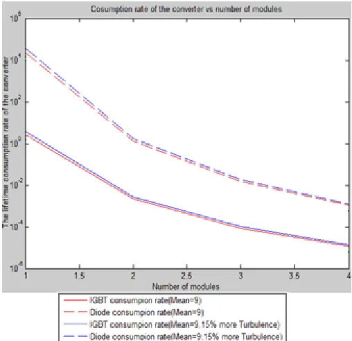
Figure 6shows the lifetime consumption rate of the diode and IGBT for different number of parallel modules. As it is obvious in the figure, the lifetime consumption rate of the diode and IGBT is decreased exponentially by increasing number of parallel modules.

Figure 6. Lifetime consumption rate of IGBT and Diode versus the number of the parallel modules

CONCLUSION

range has been used and the lifetime fluctuations of the wind speed have been modelled.

The overall lifetime of the power electronic modules for different number of parallel modules was estimated by electrical losses of the converter and the thermal data of the devices.

This study also shows that with the same wind mean wind speed the lifetime of converter for similar number of the parallel IPMs is higher for less wind turbulence value

One of the limitations in this study is the empirical model of lifetime estimation of converter that used. It is possible the empirical model is not accurate model for low amplitude, high number thermal cycles from the AC waveform. But as this model had been used for all the simulations with all different conditions, the best way to interpret the data is to compare all of results together.

REFERENCES

[1] European Reneable Energy Council, 2008, “Renewable Energy Technology Roadmap 20% by 2020,” European Reneable Energy Council, Brussels.

[2] Department of Energy and Climate Change, 2011, “UK Renewable Energy Roadmap,” Department of Energy and Climate Change, London.

[3] G. Wilson, D. McMillan and G. Ault, 2012, “Modelling the effects of the environment on wind turbine failure modes using neural networks,” in International Conference on Sustainable Power Generation and Supply (SUPERGEN 2012), Hangzhou.

[4] F. Spinato, P. Tavner, G. J. W. van Bussel and E. Koutoulakos, 2009, “Reliability of wind turbine subassemblies,” IET Renew. Power Gener, vol. 3, no. 4, pp. 387-401.

[5] M. Parker and C. Soraghan, 2013, “A Comparison of Converter Lifetime Between Horizontal- and Vertical-axis Wind Turbines,” in IET Renewable Power Generation Conference, Beijing .

[6] R. Zehringer, A. Stuck and T. Lang, 1, 1998, “Material Requirements for High Voltage, High Power IGBT Devices,” Solid-State Electronics, vol. 42, no. 12, pp. 2139-215.

[7] S. Yang, D. Xiang, A. Bryant, P. Mawby, L. Ran and P. Tavner, 2010, “Condition Monitoring for Device Reliability in Power Electronic Converters: A Review,”

IEEE Transactions on Power Electronics, vol. 25, no. 11, pp. 2734-2752.

[8] T. Ishihara, A. Yamaguchi and M. Sarwar, , 2012 “A Study of the Normal Turbulence Model in IEC 61400-1,” WIND ENGINEERING , vol. 36, no. 6, pp. 759-766.

[9] I. Van der Hoven, 1957, “Power Spectrum Of Horizontal Wind Speed In The Frequency Range From 0.0007 To 900 Cycles Per Hour,” Journal of Meteorology , vol. 14, no. 2, p. 160–164.

[10] T. Burton, D. Sharpe, N. Jenkins and E. Bossanyi, 2002, “The Wind Resource,” in Wind Energy Handbook, JOHN WILEY & SONS, LTD, pp. 11-40.

[11] O. Senturk, S. Munk-Nielsen, R. Teodorescu and L. Helle, 2011, “Electro-thermal modeling for junction temperature cycling-based lifetime prediction of a press-pack IGBT 3L-NPC-VSC applied to large wind turbines,” in IEEE Energy Conversion Congress and Exposition , Phoenix. [12] F. Fuchs and A. Mertens, 2011, “Steady State Lifetime

Estimation of the Power power semiconductors in the rotor side converter of a 2 MW DFIG wind turbine via power cycling capability analysis,” in 14th European Conference on Power Electronics and Applications (EPE 2011), Birmingham.

[13] A. Grauers and P. Kasinathan, 2004, “Force Density Limits in Low Speed PM Machines Due to Temperature and Reactance,” IEEE Transaction on Energy Conversion,

vol. 19, no. 3, pp. 518 - 525.

[14] A. Wintrich, U. Nicolai, W. Tursky and T. Reimann, 2004, “Application Manual Power Semiconductors,” SEMIKRON International GmbH, Nurembergx.

[15] I. Kovačević, U. Drofenik and J. Kolar, 2010, “New Physical Model for Lifetime Estimation of Power Modules:,” in International Power Electronics Conference (IPEC), Sapporo.

[16] C. Yin, H. Lu, M. Musallam, C. Bailey and C. Johnson, 2008, “A Prognostic Assessment Method for Power Electronics Modules,” in 2nd Electronics System-Integration Technology Conference, ESTC, Greenwich. [17] M. Held, P. Jacob, G. Nicoletti, P. Scacco and M.-H.

Poech, 1997, “Fast Power Cycling Test for IGBT Modules in Traction Application,” in International Conference on Power Electronics and Drive Systems.

[18] A. Niesłony, 2009, “Determination of fragments of multiaxial service loading strongly influencing the fatigue of machine components,” Mechanical Systems and Signal Processing, vol. 23, no. 8, pp. 2712-2721.