On the functional relationship between biodiversity and economic value

(1)

A P P L I E D E C O L O G Y Copyright © 2020 The Authors, some rights reserved; exclusive licensee American Association for the Advancement of Science. No claim to original U.S. Government Works. Distributed under a Creative Commons Attribution NonCommercial License 4.0 (CC BY-NC).

On the functional relationship between biodiversity

and economic value

Carola Paul1,2*, Nick Hanley3, Sebastian T. Meyer4, Christine Fürst5, Wolfgang W. Weisser4, Thomas Knoke1

Biodiversity’s contribution to human welfare has become a key argument for maintaining and enhancing bio-diversity in managed ecosystems. The functional relationship between biobio-diversity (b) and economic value (V) is, however, insufficiently understood, despite the premise of a positive-concavebVrelationship that dominates scientific and political arenas. Here, we review how individual links between biodiversity, ecosystem functions (F), and services affect resultingbVrelationships. Our findings show thatbVrelationships are more variable, also taking negative-concave/convex or strictly concave and convex forms. This functional form is driven not only by the underlyingbFrelationship but also by the number and type of ecosystem services and their potential trade-offs considered, the effects of inputs, and the type of utility function used to represent human preferences. Explicitly accounting for these aspects will enhance the substance and coverage of future valuation studies and allow more nuanced conclusions, particularly for managed ecosystems.

INTRODUCTION

The destructive power of humankind on natural ecosystems and the organisms living therein is well documented (1). During the past two decades, awareness that species extinction, habitat loss, and popula-tion decline in both natural and managed ecosystems may adversely

affect human well-being has increased (2,3). Economic valuation has

emerged as an important tool to illustrate this link between nature and

human welfare (3,4). Increasing public attention has spurred interest

in and funding of a number of joint academic and policy initiatives such as the European Biodiversity Strategy to 2020, Aichi targets, Sus-tainable Development Goals, and the IPBES (Intergovernmental Plat-form on Biodiversity and Ecosystem Services). These initiatives largely

build on the value of ecosystem services concept (Table 1) (3,5) and the

CICES (Common International Classification of Ecosystem Services) cascade (6), in which aspects of biodiversity are valued indirectly as the foundation of ecosystem functioning and service provision (Fig. 1) [see reviews (7–9)].

Evidence from biodiversity–ecosystem function research points

toward an increase in ecological benefits with higher levels of

bio-diversity (10,11). This relationship has also been hypothesized for

the link between biodiversity and economic value. For example,

Seddonet al.[(12), p. 7] conclude“(…) that by maximizing species,

functional and phylogenetic diversity we maximize an ecosystem’s

value over the long term.”However, empirical studies investigating

functional biodiversity (b)–economic value (V) relationships are

rare, while the methods and concepts of economic valuation applied

are very heterogeneous. This refers, inter alia, to the concept of“

bio-diversity”(discussed in more detail below), ranges of biodiversity

levels considered, as well as the type of ecosystem services, their

in-teractions, and the valuation method used. These complexities leave us with an incomplete and unsatisfactory understanding of the func-tional relationships between biodiversity and economic value.

Despite lacking evidence, the implicit assumption of a positive re-lationship between biodiversity and economic value prevails in the

political arena (4,13). Gaining an improved understanding ofbV

re-lationships and the conditions affecting possible functional forms will be crucial to provide a better scientific footing for future valuation studies, thereby informing future private and public ecosystem man-agement decisions. The objective of this study is therefore to set out a

range of possiblebVrelationships based on theoretical considerations

backed up with empirical evidence. Our research is guided by the following question: What are the functional relationships between biodiversity and economic value? We argue that these links may be more complex and more variable than generally assumed. Our focus

is on revealing the conditions under which specific functionalbV

re-lationships may be expected.

Following the definition by Pascualet al.(14), we will refer to“

eco-nomic value”as the anthropocentric and instrumental values,

quanti-fied by direct or indirect use and nonuse values of biodiversity, which we describe in more detail in the following section (see also Table 1). We follow the premise that the economic value of biodiversity may be affected by many intermediate steps, as illustrated in Fig. 1. We build on the three-step effect CICES cascade as a mechanistic model to link economic value to biodiversity. We review how methodological choices may affect the functional relationship of links between bio-diversity, ecosystem functions, services, and values and how these

may ultimately affect the expectedbVrelationships.

We start by describing the cascade model, providing a brief re-view of individual links along the cascade. These sections draw on an extensive body of biodiversity–ecosystem functioning and eco-system service research. The next section discusses important shapes

of possiblebVrelationships (Fig. 2), which have been derived from

stylized mathematical functional relationships informed by theoretical and empirical evidence. These relationships are conceptual in nature and are useful in illustrating how economic value may be influenced by changes in biodiversity. Last, we outline how the conditions

iden-tified to affectbVrelationships could be incorporated in future

valu-ation studies. With this study, we hope to contribute to an improved 1

Institute of Forest Management, Department of Ecology and Ecosystem Management, TUM School of Life Sciences Weihenstephan, Technical University of Munich, 85354 Freising, Germany.2_{Department of Forest Economics and Sustainable Land-use}

Planning, University of Goettingen, 37077 Goettingen, Germany.3Institute of Bio-diversity, Animal Health and Comparative Medicine, University of Glasgow, Glasgow G12 8QQ, Scotland.4_{Terrestrial Ecology Research Group, Department of Ecology and}

Ecosystem Management, TUM School of Life Sciences Weihenstephan, Technical Uni-versity of Munich, 85354 Freising, Germany.5_{Institute for Geosciences and Geography,}

Department of Sustainable Landscape Development, Martin-Luther University Halle, 06108 Halle, Germany.

*Corresponding author. Email: [email protected]

on September 17, 2020

http://advances.sciencemag.org/

(2)

Table 1. Definitions used in this study (direct quotations from corresponding sources if not denoted otherwise).

Term Definition Source

Biodiversity The variability among living organisms from all sources, including inter alia terrestrial, marine and other aquatic ecosystems and the ecological complexes of which they are part. Biodiversity includes diversity within species, between species and between ecosystems

(5) following the 1993 Convention on Biological Diversity

Ecosystem function

The transfer of energy, material, organisms or information among the components in an ecosystem (25) based on (24)

Ecosystem service

The aspects of ecosystems utilized (actively or passively) to produce human well-being (13)

Value The contribution of an action or object to user-specified goals, objectives or conditions (5)

Utility A measure of satisfaction or relative preference (3)

Intrinsic value Inherent value that is the value something has independent of any human experience or evaluation. Such a value is viewed as an inherent property of the entity (e.g. an organism) and not ascribed or generated by external valuing agents (such as human beings)

(14)

Instrumental value

The value attributed to something as a means to achieve a particular end such as human well-being (14)

Economic value Economists group values in terms of“use”or“nonuse”value categories, each of which is associated with a selection of valuation methods.Use valuescan be both direct and indirect and relate to the current or future (option) uses.Direct usevalues may be“consumptive”(e.g. drinking water) or“nonconsumptive” (e.g. nature-based recreational activities).Indirect use valuescapture the ways that people benefit from something without necessarily directly seeking it out (e.g. flood protection).Nonuse valuesare based on the preference for components of nature’s existence without the valuer using or experiencing it and are of three types:existence value, altruistic value and bequest value

(14)

Stated preference Consumer preferences are understood through questions regarding WTP or willingness to accept (3)

Uncertainty A broad concept meaning limited knowledge about the future, present, and past. Knight (60) distinguishes between risk (events can be quantified by probabilities) and uncertainty (events cannot be quantified by probabilities). Walkeret al.(61) define five levels of uncertainty: (i) clear enough future (with sensitivity information); (ii) alternate futures with probability; (iii) alternate futures can be ranked according to likelihood; (iv) multiplicity of alternate futures, no ranking possible; (v) unknown future. Our examples mainly assume type 2 uncertainty; in Discussion, we also mention studies dealing with type 4 uncertainty

Based on (60,61)

WTP The maximum income that an individual would be willing to give up to gain something good, such as improvement in environmental quality, or to avoid something bad, such as a decrease in

environmental quality

(113)

Willingness to accept

The minimum monetary compensation that an individual would be willing to accept to forgo something good, such as improvement in environmental quality, or to put up with something bad, such as a decrease in environmental quality

(113)

Revealed preference

A method to assess possible value options or to define utility (consumer preferences) based on the observation of consumer behaviour [estimated for example through the travel cost method, or hedonic pricing e.g. by using real estate prices as a surrogate market for clear air or aesthetic views]

(3) (extended)

Production function

A function used to estimate how much [biodiversity and/or] a given ecosystem service (e.g. regulating service) contributes to the delivery of another service or commodity which is traded on an existing market

(5)

Externality A consequence of an action that affects someone other than the agent undertaking that action and for which the agent is neither compensated nor penalized through the markets. Externalities can be positive or negative

(5)

Social costs and benefits

Costs and benefits as seen from the perspective of society as a whole. These differ from private costs and benefits in being more inclusive (all costs and benefits borne by some member of society are taken into account) and in being valued at social opportunity cost rather than market prices, where these differ; sometimes termed“economic”costs and benefits

(5)

Benefit transfer Economic valuation approach in which estimates obtained (by whatever method) in one context are used to estimate values in a different context

(5)

Insurance value Decrease of the risk premium due to a (marginal) change in the level of biodiversity. The risk premium is the reward required by a risk-averse person for accepting a higher risk or, in other words, the amount of money that generates the same utility (for a risk-averse decision-maker) between the two situations of receiving for sure the expected return minus the risk premium or facing the risky (random) return

Own definition inspired by (114)

Option value The WTP a certain sum today for the future use of an asset (115)

(3)

Fig. 1. Underlying cascade and types of values for linking biodiversity with economic value.Taken from Potschin and Haines-Young (6) with small alterations and extensions. Blue boxes follow the indirect valuation pathway (solid lines), and yellow boxes include direct valuation (dashed lines) or combinations of both. For def-inition of terms, see Table 1. Abbreviations used in blue boxes are also used for mathematical representations in the text, Table 2, and Supplementary Methods.

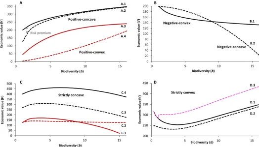
Fig. 2. Plausible biodiversity–economic value(bV) relationships derived from theoretical considerations and empirical examples reviewed here.See Table 2 and Supplementary Methods for detailed description and assumptions of example relationships depicted here. (AtoD) Economic value is given in monetary units, and biodiversity is given in number of species (see Supplementary Methods for numerical examples). For A.3, thexaxis has to be multiplied by a factor of 100.

(4)

understanding ofbVrelationships, thus informing future develop-ment and application of interdisciplinary valuations studies, oriented toward a better means of including biodiversity in private and public decision-making.

A CASCADE LINKING BIODIVERSITY TO ECONOMIC VALUE The value of biodiversity has been described as the result of a cascade of links from biodiversity (b) through ecosystem functions (F) to

eco-system services (S) to economic value (V) (Fig. 1) (6). Costanzaet al.

(4) argue that a cascade is not suitable for representing complex,

non-linear relationships and feedbacks between biodiversity and economic value. However, we are convinced that a cascade model is helpful for investigating how these relationships could be untangled and how

they contribute to the shape of the overallbVrelationship, especially

in cases where there are nonlinearities. We extend the cascade depicted

in Fig. 1 according to suggestions by Bartkowski (15) to consider

as-pects of uncertainty. We first describe the current understanding of these individual links, which will allow us to deduce the resulting shape

of thebVrelationship, which is our primary focus.

Biodiversity–ecosystem function relationships

The term biodiversity was coined by Wilson (16) as a shortened

ver-sion of“biological diversity.”At first glance, the concept can be simple:

“biodiversity is the sum total of all biotic variation from the level of

genes to ecosystems”(Table 1) (17). While these simplified

defini-tions are still frequently used in economic valuation (15), the

multi-dimensional nature of biodiversity as understood in ecology requires a

range of different metrics to describe its different aspects (17). Modern

ecological research considers the number of species (18),

abundance-weighted species richness and evenness of species distributions (19),

functional diversity (i.e., the diversity in functional attributes or traits

in a community) (20), phylogenetic diversity (i.e., the evolutionary

re-latedness in a community) (21), and genetic and phenotypic diversity

among and within species (22). Most commonly used as a measure of

biodiversity is the number of species, which we will use for simplicity in the following text and in the empirical examples, when not noted otherwise.

The persistence of ecosystems requires the continuous flow of

energy and the recycling of matter (23). The transfer of energy, material,

organisms, or information among the components in an ecosystem is

called an ecosystem function (Table 1) (24,25).

Classically, biodiversity research is interested in understanding the abiotic and biotic drivers of the diversity of organisms in an ecosystem.

The relatively young field of biodiversity–ecosystem functioning (bF)

research emerged around 1990. This field considers biodiversity itself as a driver of ecosystem properties, thus asking questions about the functional importance of biodiversity (26). The past three decades

have seen an increased interest in this question (7,27). Biodiversity

experiments that manipulate species richness while excluding con-founding effects are an important tool to test causal relationships

between biodiversity and ecosystem functions (28). Early and very

influential biodiversity experiments were set up in the United States

in Cedar Creek, MN (29) by the BIODEPTH consortium in Europe (30)

and in the United Kingdom (31). These and subsequent biodiversity

experiments [the Jena Experiment described in (32)] have resulted in

more than 570 independent manipulations of species richness that now form the foundation of our understanding of the effect of bio-diversity on ecosystem functions.

The main conclusion frombFresearch of the past decades is that a

low diversity in an assemblage is associated with a lowered mean level of many ecosystem functions and is often associated with an increase

in the coefficient of variation of the level of the functions (11,33,34).

Several meta-analyses support this conclusion in terrestrial [e.g.,

(35,36)] and marine (37) ecosystems.

Species richness and ecosystem function relationships typically are positive-concave curves that frequently saturate at low levels of species richness, e.g., when three to six species are present in the system (30). These saturating relationships have been taken as support for the

re-dundancy hypothesis (38,39), which proposes that high functioning

can be achieved with only a few species. However, redundant species may contribute to maintaining ecosystem functions when other spe-cies are lost or under changing environmental conditions (40), referred

to as an ecological insurance effect (40,41). A turnover in the identity

of species contributing to a particular function may increase the

cu-mulative number of species sustaining functioning over time (42,43).

Last, when considering multiple functions simultaneously, the num-ber of species contributing to ecosystem multifunctionality is generally

higher than the number of species needed for single functions (44,45).

Biodiversity experiments are deliberately conducted under con-trolled conditions to investigate the effects of biodiversity independent of other confounding factors. This has sparked a long-standing debate about the questions of whether, and under what conditions, results from these biodiversity experiments can be transferred to the natural

world and to managed ecosystems (46,47). In these natural or

man-aged“real-world”systems, there are many environmental and

man-agement factors that are drivers of ecosystem functions in addition to

and interacting with biodiversity (48). Consequently, building onbF

research, we may thus assume that the ecosystem functionFdepends

on biodiversity (b) and may also depend on human inputs and

man-agement (i), such as fertilizer or pesticides.

F¼fðb;iÞ ð1Þ

Ecosystem functions and ecosystem services

The idea of“ecosystem services”has undergone a process of

approach-ing an appropriate definition (Table 1) [e.g., (3,5,13,49,50)]. This can

now be summarized as contributions to human well-being that people can experience from natural processes, patterns, and structures (i.e., ecosystem functions sensu lato). Generally speaking, all definitions cover the different aspects of ecosystems from the perspective of human

well-being (51). This implies that an ecosystem function can only be a

service if a demand is identified. Ecosystem functions would thus form

the capacity of ecosystems to provide services (52). This indicates that all

services are related to functions, while, vice versa, ecosystem functions that do not result in a service exist. This strong link between ecosystem functions and services might not be fully applicable for cultural services, which often include human interventions to create a service [e.g.,

cul-tural landscapes and recreational values (53)]. Social and behavioral

sciences have largely worked independent of the service concept to

an-alyze the importance of nature’s cultural services for people. However, it

has also been shown that models can link cultural and aesthetic services with functions [i.e., ecosystem structures and processes from a land-scape perspective (54)]. Cultural services may then be integrated into

the concept of ecosystem services (55), and indicator sets have been

sug-gested in the context of the national-level mapping [e.g., (56)]. For our present purposes, we assume that consistent and quanti-fiable links exist between ecosystem functions and services, which

(5)

may be used as a basis for valuation. We exemplify these links for a

single or bundled ecosystem service(s),S, which is dependent on one

or more ecosystem functions (see Eq. 1) and on an indicatorP,

show-ing if and how strongly this ecosystem function is in demand.

S¼fðF;PÞ ð2Þ

Pforms a link to valuation. It may be represented by a price or social benefits for one unit of an ecosystem function, as described below.

Valuation of ecosystem services and biodiversity

To provide an analytical framework, we focus on how changes in

biodiversity-related ecosystem functions and services affect peoples’

utility either directly or indirectly. Utility is a concept for measuring

peoples’degree of satisfaction and thereby the subjective value people

assign to something in making choices. A utility function is a device that helps us predict how people will make choices between alterna-tives and gives one way of representing human well-being. A benefit is a specific advantage being valued or its contribution to overall utility, for example, the opportunity for outdoor recreation. We refer to eco-nomic valuation as an attempt to measure human preferences for a good. Theoretically, economic value is the total area under the de-mand curve for a good or service (see fig. S1A), but this information is not usually available for many aspects of biodiversity and the ser-vices it supports.

In Fig. 1, we differentiate between two ways of estimating the con-tribution of biodiversity to economic value, referred to as direct and indirect. First, people may obtain direct benefits from the presence, diversity, and abundance of organisms or ecosystems. For example, people can experience greater utility from walking in woodlands with more bird species than fewer species and may be happier knowing that a new marine protection area is conserving cold water corals, even if they themselves cannot visit the corals. These aspects generate a mix of use and nonuse values, the latter often being distinguished into

exis-tence, bequest, or altruistic values [see Table 1 and (57)]. These values

directly affect peoples’utility to varying degrees, in which interperson

variability is referred to as preference heterogeneity.

Building further on the cascade approach, we can also quantify the benefits of biodiversity in an indirect way. For instance, when higher species diversity results in an increased net primary production (NPP) and therefore enhances provisioning and/or regulating services or when biodiversity provides pest control affecting marketable food products or if high overall forest plant diversity is needed to obtain

specific pharmaceutically valuable species, then peoples’utility is

in-directly increased by these effects (see solid lines and blue boxes in Fig. 1). This type of valuation builds on all steps along the cascade using ecosystem services as an intermediate link between the ecological and economic context. Ecosystem services can be characterized as market-based private goods (e.g., timber outputs), as nonmarket-based quasi-public goods (e.g., the opportunity for recreation in forests), and as positive externalities (e.g., carbon sequestered by means of forestry) (Table 1). For many of the biodiversity-dependent goods, markets do not exist, meaning that market prices cannot be used to measure the value of increases in their supply.

For both types of valuation—the direct and indirectbVapproaches

(both dashed and solid lines in Fig. 1)—the valuation of nonmarket

goods may build on among other things: (i) the avoided (social) costs when using ecosystem structures and processes rather than alternatives,

(ii) the changes in the service’s market value caused by a nonmarket

service serving as productive inputs (e.g., the effects of pollination

on crop outputs) (58), or (iii) peoples’willingness to pay (WTP) for

changes in the level of biodiversity or for an affected service. WTP attempts to quantify the expected utility experienced by a person from consuming a certain good or receiving a specific service (59).

As Bartkowski (15) shows, estimating“uncertain-world values”

(depicted in the upper yellow box and upper dashed lines in Fig. 1) is another important aspect where biodiversity is indirectly linked to notions of economic value. Here, we consider two facets of uncertainty connected to economic value. Uncertainty relates first to the fluctu-ation of services provided by a system around an estimated mean. Second, uncertainty may also be associated with potential discovery of additional species and their so far disregarded values, creating a WTP for options associated with biodiversity-rich ecosystems. Both concepts require that fluctuations or probabilities may be measurable and appropriately assigned. Such a situation is often referred to as

de-scribing“risk”(60) or as level 2 uncertainty, where alternate futures

with identifiable probabilities exist (Table 1) (61). However, these

es-timations, for example, of standard deviations of provided functions or probabilities of discovery also involve high uncertainty. Therefore, we here use risk and Knightian uncertainty interchangeably following

Bikhchandaniet al.(62), assuming that some quantification of

uncer-tainty is needed to understand its economic consequences.

One way of economically integrating these uncertain-world values is by a concave utility function characterized by diminishing marginal utility. On the basis of this utility curve, an insurance value may arise if economic return fluctuations are reduced by growing a higher variety of crop species, whose return fluctuations are independent or nega-tively correlated. A reduction in return fluctuations, excluding any effects of crop diversity on the expected (average) return, will increase utility for risk-averse persons, while he or she will require a reward

(a“risk premium”) for accepting higher levels of risk (Table 1) (62).

Therefore, a risk-averse farmer would benefit from using a higher agrobiodiversity of crop species as a production input as well as a risk

hedging strategy (63). Building on the simple proverb of“don’t put all

your eggs in one basket,”the farmer would require a smaller risk

pre-mium when using higher agrobiodiversity for production. Baumgärtner

(64) and Finger and Buchmann (65) estimated an insurance value of

biodiversity as the decrease of the risk premium when biodiversity increases by one unit.

Concerning our second example of uncertainty, biodiversity may

also offer option values (Table 1) (15). Higher levels of biodiversity

may, for instance, provide future but currently unknown commercial opportunities in an uncertain world, such as the potential use of spe-cific species for pharmaceutical products or using biodiversity as a library on genetic information for future screening (66). A large frac-tion of prescripfrac-tion drugs are derived from natural products, while genetic information is also important for plant breeding.

Bioprospect-ing attempts to realize this potential (67). Consequently, biodiversity

generates an option value concerning currently unknown future benefits

(15). In addition, the economic theory of real options brings an aspect

of flexibility into consideration (68). For example, one can postpone

decisions on invasive species control to obtain better information to

improve policy responses (69). In natural resource management, the

value of these options depends on the degree of flexibility they provide

for decision-makers (70), where flexibility is better facilitated by

resist-ant compared to vulnerable ecosystems (71). Empirical evidence also suggests that (economic) resistance to shocks may depend on the level

of biodiversity in some situations (72).

(6)

RESULTING SHAPES OF BIODIVERSITY–ECONOMIC VALUE RELATIONSHIPS

On the basis of this economic background of valuation, we postulate

that the main contribution of biodiversity to economic value (V) is

associated with facilitating and supporting ecosystem services. Utility

(U) is thus created indirectly asU(S) (Fig. 1, solid lines). The

contri-bution of biodiversity is also a direct one, i.e.,U(b), when people obtain

benefits from the presence, diversity, and abundance of organisms or ecosystems (lower dashed line in Fig. 1). Summarizing both types of valuation, economic value may then be described as

V ¼fðUðS;bÞÞ ð3Þ

Given the cascade,F=f(b,i)→S=f(F,P)→V=f(U(S)) (Fig. 1), we will focus mainly on the indirect contribution of biodiversity to economic value, as this contribution may be established using the well-researched biodiversity–ecosystem function relationships. We derive four hypotheticalbVrelationships illustrated in Fig. 2. The relationships include positive-concave and positive-convex (Fig. 2A), negative-concave and negative-convex (Fig. 2B), and strictly concave (Fig. 2C) and (quasi-) or strictly convex (Fig. 2D) functional forms. We suggest that the functional relationships are driven by five main conditions: (i) the type ofbFrelationship, (ii) the number and type of ecosystem services considered, (iii) the trade-offs between services or between risk and return, (iv) whether effects of“synthetic”inputs are considered, and (v) the type of utility function used to represent human preferences.

For each functional form, we discuss the conditions under which it may be expected and how a potential mathematical formulation may look (Table 2). The rationale for each mathematical representation and the underlying assumptions are described in more detail in Sup-plementary Methods. We will then discuss how well these relation-ships are supported by empirical evidence. Our starting point will

be the most frequently assumed positivebVrelationship.

Positive-concave or positive-convex relationships

A positive-concave relationship between biodiversity and economic values (Fig. 2A) means that economic value increases with additional species in the ecosystem at a diminishing rate. The response in eco-nomic value per additional unit of biodiversity is large when starting at a low level of biodiversity and decreases for higher levels (Fig. 2A, A.1).

This relationship may result from a positive-concavebF

relation-ship, frequently observed for single ecosystem functions, such as

NPP (73–75). O’Connoret al.(76) have, for example, described the

relationship between a change in species richness on biomass (hereF)

(Table 2) as a power function

FðbÞ ¼a_bb _ð₄_Þ

withaandbbeing coefficients, defined asa> 0 and 0 <b< 1 for a positive-concavebFrelationship. Provided that a demand for the eco-system function exists and that the economic value is proportional to the ecosystem service, a positive-concavebVrelationship results. This proportional relationship builds on two main assumptions: First, the priceP(Eq. 2) attributed to each species is identical for all species, which means that the ecosystem service provided (denoted asSin Eq. 2) is considered a homogeneous good (Table 2, column“Type ofSgood”). This condition would, for example, apply to carbon

sequestration where there are no differences in the value of a ton of carbon sequestered by different species [e.g., (74)]. The commercial market price for hay might, however, differ between grassland species because of differences in quality and consumer preferences (Table 2) [e.g., (77)]. Second, the linear relationship betweenSandV(Eqs. 2 and 3) provides that the relative increase in satisfaction gained from receiving an additional unit ofSis constant for all levels ofS. This could be represented by a linear utility functionU(S) (Eq. 3). Such a utility function assumes that decisions are taken independently from risks (i.e., assuming risk neutrality) and wealth of the decision-makers (see Table 2, column“Human preferences”).

A recent example for a positive-concavebVrelationship is a study

by Lianget al.(75) (Fig. 3A). On the basis of a positive-concave

rela-tionship between biodiversity and NPP derived from experimental

plots, Lianget al.(75) suggest a high commercial wood value

asso-ciated with the biodiversity of species-rich forests. The underlying as-sumption is that the economic value added from forests is directly affected by, and proportional to, forest productivity (i.e., biomass pro-duction; see green triangles in Fig. 3A). Here, biomass is directly re-lated to a mean commercial value, meaning that wood is considered a homogeneous good, for which quality and species identity are not ex-plicitly considered.

Similarly, Hungateet al.(74) found a positive-concavebVbased

on the social costs of carbon (Table 1) estimated for an increasing num-ber of species in pasture systems (see magenta circles in Fig. 3A). While

these studies focus on a single ecosystem service—wood production

and carbon storage—Costanzaet al.(73) used an aggregated value,

where ecoregion-specific NPP values were coupled with a benefit

trans-fer function based on an earlier study by Costanzaet al.(78) (yellow

circles in Fig. 3A). Using this type of aggregation, trade-offs between

services are assumed to be absent (see Table 2, column“Trade-offs/

social costs or benefits”), and quite different individual preferences

are aggregated to derive economic values (79).

The studies mentioned above applied linear utility functions, and this rather strong assumption has been relaxed by Finger and

Buchmann (65) using a positive-concave utility function to assess

av-erage returns from grassland yields and their variance (blue diamonds in Fig. 3A). This utility function accounts for the effects of uncertainty

in ecosystem service provision on peoples’preferences. Under the

presence of uncertainty, the notion of“expected utility,”E[U(S)], is

used. Given a concave utility function, the expected utility of the same average economic return then increases with decreasing variance.

Finger and Buchmann’s study assumed a positive-concavebF

relation-ship for grassland biomass yield and a negative-convexbFrelationship

for the variance of yield, which is in line with findings from biodi-versity experiments (11). This constitutes two positive effects (a double dividend) of increasing biodiversity, here quantified by Shannon di-versity index, namely, increased mean provision and reduced variabil-ity of the studied service. Combining a concave utilvariabil-ity function with a

concavebFreinforces the positive-concavebVrelationship rather than

altering the general relation (Table 2 and Fig. 2A, A.2).

Concave, positive relationships have also been found for the eco-nomic value of additional species in the pharmaceutical industry (80).

As the functional relationship published by Simpsonet al.(80) shows

(Fig. 3B), stochastic considerations—known as sampling effects inbF

research—may constitute a positive impact of biodiversity on economic

value (Fig. 2A, red solid line, and Table 2, A.3). When species richness increases, the probability of finding a new species of value for the phar-maceutical industry rises.

(7)

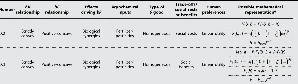
Table 2. Description of conditions (columns) for hypothesized biodiversity (b)–economic value (V) relationships (lines) as depicted in Fig. 2.Numbers in the first column refer to denomination of functional relationships in Fig. 2 (bF, biodiversity-function relationship;S, ecosystem service). For further explanation and derivation of mathematical functions, see the Supplementary Materials. In our example mathematical representations, we refer to biodiversity as the number of species (see the Supplementary Materials for numerical examples).

Number bV

relationship

bF

relationship

Effects drivingbF

Agrochemical inputs

Type of

Sgood

Trade-offs/ social costs or benefits

Human preferences

Possible mathematical representation*

Relationship of

cascade affected bF bF bF-FS SV SV SV

A.1

Positive-concave Positive-concave

Biological

synergies† No Homogeneous No Linear utility

V(b) =PF(b)

F(b) =abb0 <b< 1

A.2

Biological synergies/ stochastic (averaging effect)

No Homogeneous No Concave utility (risk averse)

V(b) =PF(b)0_:5_PF₍g_b₎ var(PF(b))

F(b)

¼E[abb];F(b) =abb

0 <b< 1,g> 0

A.3

Stochastic

(sampling) effect No

Assumed as

homogeneous No Linear utility

V(b) =PF(b)

F(b) = 1−(1−p)b

P> 0

A.4

Positive-convex Positive-convex

Biological

synergies No Homogeneous No Linear utility

V(b) =PF(b)

F(b) =abbb> 1

B.1

Negative-convex Negative-convex

Biological

synergies No Homogeneous No Linear utility

V(b) =PF(b)

F(b) =abbb< 1

B.2 Negative-concave

Negative-concave No synergies No Homogeneous No Linear utility

V(b) =PF(b)

F(b) =a(1₋(bm+ 1)−bbb)

C.1 Strictly concave

Negative-concave

Stochastic (averaging) effect

No Homogeneous Risk return Concave utility (risk averse)

V(b)¼PF(b)0:5 g

PF(b) var(PF(b)) F(b)

¼E[a(1(bm+ 1)bbb)] F(b) =a(1−(bm+ 1)−bbb)

b> 1,g> 0

C.2 Strictly

concave Negative-convex

Biological synergies/ stochastic (averaging)

effect

No Homogeneous Risk return Concave utility (risk averse)

V(b) =PF(b)0:5 g

PF(b) var(PF(b)) F(b)

=E[abb];F(b) =abb

b< 0,g> 0

C.3 Strictly

concave Positive-concave

Biological

synergies No Heterogeneous Various prices Linear utility

V(b)¼P(b)F(b)

F(b) =abb

0 <b< 1

C.4 Strictly concave

Positive-concave +

negative-concave

Biological

synergies No Homogeneous TwoS Linear utility

V(b) =P1F1(b) +P2F2(b)

F1(b) =a1bb1

F2(b) =a2(1−(bm+ 1)−b2bb2)

0 <b1< 1,b2> 1

D.1 Strictly

convex Positive-concave

Biological synergies

Fertilizer/

pesticides Homogeneous No Linear utility

V(b,i) =PF(b,i)

F(b,i) =a

(

b bmb+

(

1

b bm

)

wi

)

b

b=bmaxi−ϑ

continued on next page

(8)

As a third form of a positivebVlink, we conceptualize a positive-convex relationship (Fig. 2A, A.4). For this case, the increase in econom-ic value per additional biodiversity unit would be increasingly larger at a higher biodiversity level. Such a relationship could arise from

positive-convexbFrelationships, as hypothesized by Moraet al.(81), for which

empirical evidence is so far lacking. Given a homogeneous good and a

linear utility function, a positive-convexbFlink would translate into a

positive-convexbV(Table 2, A.4).

In conclusion, the evidence collected above suggests a

positive-concavebVrelationship under certain conditions. These include the

valuation of a single ecosystem service of interest or the absence of trade-offs between multiple ecosystem services or risks and returns, strong ecological synergies and/or sampling effects, and the consideration

of a homogeneous ecosystem output—such as carbon sequestration—for

which species identity and quality are less relevant. It mostly requires a linear utility function or a concave utility function when variability of

the level ofFis considered.

Negative-concave or negative-convex relationships

A positivebFlink was a precondition for the results presented above.

However, ecosystem functions are not always positively linked with spe-cies diversity, possibly resulting in a negative, either concave or convex

bVrelationship (Fig. 2B). For instance, Costanzaet al.(73) showed in an

empirical study of various ecoregions of North America that the NPP of low-temperature regions—as opposed to high-temperature regions— was negatively correlated with species richness. Combining NPP with an economic value function that considers multiple services created a

negativebVrelationship for these low-temperature regions. In

agree-ment with this finding, a recent study by Sandauet al.(46) found

neg-ativebFrelationships for specific conditions in a grassland experiment,

where colonization from the surrounding species pool was allowed.

Hence, a negativebFmay turn a positive-concave or positive-convex

relationship into a negative one, even when assuming a homogeneous service good, a linear utility function, and the absence of trade-offs (Table 2, B.1).

In addition to these rather scarce empirical examples for a negative

bF, we may theoretically expect these relationships in the absence of

biological synergies. This means that we would exclude any beneficial

interactions between species, which are the mechanistic basis for a

pos-itivebFrelationship. This could, for example, be the case when growing

crops on separate parcels of a field, thus avoiding the higher complexity of mixed, e.g., intercropping, systems. Growing various parcels of dif-ferent crops, including those with lower NPP, will inherently lead to a lower average value for this ecosystem function as compared to a mono-culture of the most productive species. In the absence of biological

syn-ergy and risk aversion, this would lead to a negativebVrelationship

(Table 2, B.2).

Strictly concave relationships

Strictly concave biodiversity–economic value relationships (Fig. 2C)

may be found if assumptions deviate from those, described for

positive-concavebVrelationships in terms of (i) a utility function accounting

for risk aversion (Table 2, relationships C.1 and C.2), (ii) heterogeneous ecosystem service goods (C.3), or (iii) if trade-offs among multiple services exist (C.4).

As described in the earlier section, risk-averse persons may benefit from a statistical averaging effect associated with biodiversity, which decreases the variability of services and thus enhances expected utility. The portfolio effect is among the main causes for a positive influence

of species diversity on the stability of economic returns (65), leading to

a positive-concave relationship for risk-averse decision-makers (see Table 2, A.2). However, this provides that there is a double dividend effect, namely, a reduction of risk plus a positive effect of biodiversity on the expected return, for example, through increased yields. If the posi-tive effect of biodiversity on expected return is excluded, accounting for the resulting trade-offs between (economic) risk and expected (average) return, the relationship may turn from a positive-concave to a strictly

concavebVrelationship. This can be exemplified by a stylized farm

growing crops on separated parcels (as described above). Therefore, species interactions among crops are largely excluded while allowing efficient agricultural management. Adding additional species to such a land-use portfolio will lead to a strong initial decrease in the standard deviation of economic returns, provided that the return of the different crops is not perfectly correlated [see example in fig. S2 (pink symbols)]. With higher numbers of admixed crop species, this decrease in standard deviation of returns becomes smaller. However, the expected (average)

Number bV

relationship

bF

relationship

Effects drivingbF

Agrochemical inputs

Type of

Sgood

Trade-offs/ social costs or benefits

Human preferences

Possible mathematical representation*

D.2 Strictly

Fertilizer/

pesticides Homogeneous Social costs Linear utility

V(b,i) =PF(b,i)−iC

F(b,i) =a

₍

b bmb+

(

1

b bm

)

wi

)

b

b=bmaxi−ϑ

D.3 Strictly

Fertilizer/

pesticides Homogeneous

Social

benefits Linear utility

V(b,i) =P1F1(b,i) +P2F2(b)

F1(b,i) =a1

(

bbmb+

(

1 b bm

)

wi

)

b1

F2(b) =a2(b−1)b2

b=bmaxi−ϑ

*V(b) is the economic value depending on biodiversity,b.bis the number of species in our examples.bmis the maximum biodiversity.F(b) is the ecosystem

function, depending onb.Pis an indicator for demand; in our examples, it is a price or a (saved) social cost.P(b)is an average price, depending on biodiversity,

b.E[·] is an expected value;a,b,g,w, andϑare coefficients.g> 0 quantifies the constant relative risk aversion.Pquantifies the probability for a commercial success when testing a species for pharmaceutical use.iis a human input. var(·) is the variance. †With biological synergies, we refer to the observation that two or more organisms may produce a greater result than each would achieve individually. This may be due to ecological facilitation, which benefits at least one species in terms of increased productivity, reduced physical stress or disturbance (particularly in forest ecosystems), or reduced predation. We distinguish these effects from stochastic averaging and sampling effects described in more detail in the text.

(9)

Fig. 3. Empiric examples forbVrelationships.(A) Services related to biomass production or carbon sequestration are considered. All values have been normalized between zero (minimum economic value/species richness) and 100% (maximum economic value/species richness). Yellow: Costanzaet al.(73) estimate a biodiversity (reflected by the number of vascular plants) NPP relationship for certain ecoregions in the United States and couple this function with a function to estimate aggregated economic value published earlier (78). Magenta: Annual economic value of carbon sequestration in grasslands (74) based on a medium scenario for social costs of carbon, when progressively adding grass species to a grassland monoculture [data were adopted from Hungateet al.(74)]. The authors report net present values of differences in ecosystem carbon content with an increasing number of grass species over a 50-year period (marginal values) based on social costs of carbon (112) discounted with a constant 4% discount rate. Green: Commercial forest value when species richness (per plot) varies (75). An assumed reduction by one tree species forms high and low economic values close to 100%, while a reduction to only one tree species forms the minimum (zero achievement level). Blue: Utility of commercial value of biomass yields in grasslands depending on Shannon diversity index (65). (B) Marginal and cumulative values of species for pharmaceutical bioprospecting [data are from Simpsonet al.(80)]. A probability for a commercial discovery,

P, of 0.000012 or 0.000020 for each single species and other coefficients according to Simpsonet al.(80) was assumed to compute upper bounds for marginal species net economic value according to equation 10 of Simpsonet al.(80). The numbernof species available for pharmaceutical testing was varied from 5000 to 250,000. The mathematical products of the respective marginal net economic value and the number of additional species were summed to express the functional relationship between the number of species and the cumulative net economic value in percent. (C) Insurance value of admixing natural tree species into nonnatural forests based on data taken from (85). With nonnatural forest, we refer to a forest plantation made up by a single nonnative tree species. Admixing these stands, poor in species diversity and forest structure, with native tree species [e.g., those suggested by the concept of potential natural vegetation; see, e.g., (83)] would increase naturalness. The insurance value is quantified as the decrease in risk premium (Table 1; see eqs. S7 to S13). Here, we assigned logarithmic utility to each uncertain economic return, which was subsequently averaged. If the economic risk is high (i.e., we have volatile economic return), a high risk premium and a high expected economic return are required. For example, the high risk premium required for a nonnatural forest (Norway spruce) is reduced by about€450 per hectare by integrating 7% natural tree species (European beech) [data: (85); valuation approach: (65)].

(10)

return also decreases when adding crops with lower expected return. Capturing these risk/return trade-offs in a concave utility function, as typically assumed for risk-averse people, results in a strictly concave

bio-diversity/economic utility relationship as surrogate for abVrelationship

(fig. S2, orange line, and Table 2, C.1) (82).

In addition to the purely stochastic effect described above, higher levels of naturalness, associated with enhanced native biodiversity,

may have a stabilizing effect, also referred to as“insurance value”(see

Tables 1 and 2 and Fig. 3C). For example, consider a forest plantation that is planted with either a species maximizing for productivity and profitability (e.g., spruce in Central Europe) or the natural dominant

species (referred to as“natural”) of the region (e.g., beech) or a mixture

of both (Fig. 3C). Assume a higher survival probability for the non-natural tree species in a mixed, seminon-natural forest, where a non-natural spe-cies completes the composition. This constitutes a biological synergy, which affects the stability of the economic return (72). Further assume that aspects of biodiversity are represented by an indicator of

natural-ness of forest structure (83). The proportion of the native tree species can

be considered as an indicator for naturalness following Bončinaet al.

(84). Figure 3C shows that the monetarized insurance value (see

Table 1 and the Supplementary Materials for more details) is higher for a more diverse, seminatural forest, where the native tree species stabilizes the nonnatural species, compared to a profitable, yet risky, monoculture of the nonnatural tree species. This increase in the

in-surance value constitutes a positivebVrelationship sensu Finger and

Buchmann (65) (Table 2, A.2). However, in our example, for high

proportions (more than 50%) of the natural dominant tree species, the return declines so steeply that the balance between economic re-turn and risk becomes unfavorable. In the dataset used for this ex-ample (85), the return variability in beech-dominated stands becomes high, compared to the low average economic return. Con-sequently, the trade-off between economic return and risk turns the

positive-concave into a strictly concavebVrelationship (Table 2,

C.1). Consideration of risk reduction when using multiple species

may even turn a negative-convexbFinto a strictly concavebV(as

for B.1, see Table 2, C.2).

Our second condition for strictly concave relationships is the con-sideration of heterogeneous goods (C.3), i.e., differences in the (com-mercial) quality of ecosystem functions and resulting services

produced by specific species or ecosystems. As Binderet al.(77)

out-lined, species richness alone is, from a private producer perspective, less relevant than the identity and relative abundance of species. A farmer would only select those communities that offer the highest utility for each level of species richness. In line with risk/return analysis, this could

be considered a species/value efficiency frontier. Binderet al.(77)

calculated optimal species identity and relative abundance of managed

grassland for maximizing the economic (land) value—based on the

risk-adjusted (certainty equivalent) present value of the future stream

of profits—for each level of species richness. The economic analysis

accounted for effects of species composition and interactions on hay quality, quantity, and variability, as well as differences in seed costs. It was found that while the average of compositions showed a

positive-concavebVrelationship, the economically optimized grassland

com-munities yielded a strictly concave relationship. The same functional relationship was even found for a risk-neutral decision-maker (i.e., with

a linear utility function). This important finding demonstrates thatbV

relationships strongly depend on the species identity and composition of the studied communities, particularly when taking a private producer perspective (Table 2, C.3).

Last, a third case for a strictly concavebVrelationship is

multifunc-tionality, which has been defined as the ability to integrate human pro-duction with the retention of service flows (86). This means that we focus on multiple services, which build on single or multiple functions and are subsequently valued together or separately. Biodiversity is not always positively linked with all services and their economic values be-cause of trade-offs between functions and/or services (Table 2, C.4) (45). A further complication is that multifunctionality (in terms of functions and services) itself is not a constant but changes depending on the

num-ber and identity of considered functions (45,87). In line with this

finding, the economic value attributed to multifunctionality may be expected to change, depending on the type and number of functions/ services considered. As an example, with relationship C.4 (Fig. 2C and

Table 2), we consider two services. First, we provide a negativebF

rela-tionship, characterized by an increasing rate of reduction in the level of

Fwith increasingb(Table 2, C.4). The scenario could occur, for

in-stance, if a farm grows various crops on separated parcels in a

compart-mental land-use system (88). Second, we assume a concave saturating

bFrelationship. Within a compartmental land-use concept, such abF

may apply when high compositional crop diversity reduces soil erosion. With increasing numbers of agricultural crops, the harvesting times would become more and more diversified, meaning that the area

ex-posed for erosion would be approximately proportional to1_b, where—

in an ideal case—brefers to the number of crops. The avoided soil

erosion constitutes an economic value, and aggregating both effects

results in a strictly concavebV.

In our review, we found very few examples, which account for trade-offs between services in valuation studies [see fig. S3 for one example

based on Braat and ten Brink (89)]. The actual shape of thebV

relation-ships assuming traoffs among functions and services will greatly de-pend on the valuation of individual services, given that single services are valued and subsequently aggregated. Higher values of provisioning

services, compared to those used by Costanzaet al.(73), could have

con-siderably changed their confirmed positive-concavebVrelationship

(depicted in Fig. 3A) if trade-offs were included. For example, if

maxi-mum levels of biodiversity exclude high levels of food production—so

food becomes much more valuable under increasing scarcity—the

positive-concavebVrelationship described by Costanzaet al.(73) could

become strictly concave, with a possible maximum at intermediate levels of biodiversity. This highlights the importance of a careful selec-tion of valuaselec-tion and aggregaselec-tion methods and the use of sensitivity

analyses to identify potential functionalbVrelationships.

Strictly convex relationships

A strictly convex relationship (Fig. 2D) can be interpreted as an indi-cation that higher biodiversity may compensate for greater

manage-ment intensity and vice versa. Weigeltet al.(90) demonstrate equal

and high productivity in high-diversity/low-input and low-diversity/ high-input grassland systems. Their study suggests that management intensity could substitute for diversity when high productivity is the aim. When constraining environmental heterogeneity using inputs such as fertilizer, irrigation, or pesticides, monocultures may produce very high yields (91). Under these homogenized environmental conditions, high biodiversity is not persistent. In contrast, if envi-ronmental heterogeneity is high (i.e., without homogenization), no single species will obtain maximum yield, under all conditions, due to differentiation of niches. Increasing biodiversity will then increase

yield. Combining both perspectives results in a strictly convexbF,

which may be associated with a similarbVrelationship if economic

(11)

value is proportional to productivity (Fig. 2D, D.1, and Table 2, column

“Agrochemical inputs”).

In addition, the use of plant diversity to replace expensive agricultur-al inputs suggests a higher economic vagricultur-alue from more species-rich eco-systems, if diversity is cheaper than agricultural input or if social costs associated with environmental pollution from chemical inputs may be so avoided. These interdependencies do not alter the strictly convex

shape of thebVrelationship but may change their maxima, as seen in

Fig. 2, where, in D.2, high biodiversity (right end) more than compen-sates the economic value under high agrochemical inputs (left end). Consequences of increasing the level of biodiversity such as these have rarely been investigated in an economic context, although they could be of particular interest for highly managed ecosystems. Excessive fertilizer usage implies social costs resulting from increased air and water

pollu-tion (91). Consequently, a substantial part of the economic value of

bio-diversity (agrobiobio-diversity) is the avoided cost of nitrogen pollution, for example, reducing the social costs of nitrogen (SCN). Estimates of the

SCN are variable but may be high (92). Keeleret al.(92) report a

dis-counted value of monetary damages caused by a change in N, which varied between US$0.001 and US$10 per kilogram of nitrogen.

These effects of reducing the short-term social costs of land manage-ment are important for informing the long-term perspective. Avoided soil degradation will save long-term costs of soil rehabilitation or

repla-cement (93) and may thus change the strictly convex relationship even

further in favor of more biodiverse ecosystems. To illustrate the possible effects of both biodiversity and fertilizer on agricultural yield, we ana-lyzed data for organic and conventional farms using either multi- or monocropping systems, with multicropping referring to growing more than one different crop species on the same field during one growing season [table S1; using data obtained from (94)]. In these systems, monocropping may produce higher agricultural yields than multicrop-ping systems, but only under high N inputs (fig. S4). In contrast, the multicropping system delivers relatively high agricultural production levels at a much lower N input. For example, multicropping may achieve an annual level of production of 4.4 tons per hectare with 80 kg less N input than monocropping. If we assume a very high potential SCN of US$10 per kilogram of nitrogen, saving 80-kg nitrogen by exploiting agrobiodiversity would yield a present value of US$ 800 per hectare each year. This demonstrates the importance of the idea of ecological

replacement (95) in valuing biodiversity, which may lead to a strictly

convex functionalbVrelationship.

Using this example, we can also account for other nonmarket benefits of biodiversity, for example, considering improved carbon

stor-age in more biodiverse ecosystems (74). This would lead to abV

rela-tionship, as shown in Fig. 2 (D.3). Under these conditions, more biodiverse ecosystems may actually dominate monocultures with high agrochemical inputs, from an economic value point of view.

CHALLENGES AND OPPORTUNITIES FOR FUTURE RESEARCH Our research shows that the functional relationship between bio-diversity and economic value is more variable than the well-known

and often presumed positive-concavebFrelationship. This enhanced

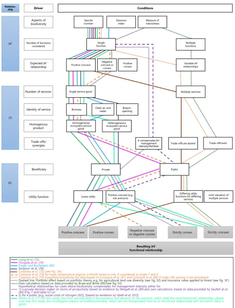
complexity arises even in simplified theoretical functional relationships, as demonstrated in Table 2. Figure 4 summarizes the identified

conditions driving possiblebVfunctional forms along the three-step

cascade (Fig. 1) and illustrates how far these conditions are covered by the empirical examples used in our review. The lines connecting dif-ferent conditions represent the selected studies reviewed here. The large

majority of empirical studies reveal positive-concavebVrelationships,

while they only cover a limited number and types of conditions. The simplified roadmap reveals that, although theoretical considerations (dashed lines in Fig. 4) and single empirical observations (solid lines) give strong arguments for strictly concave and convex relationships,

comprehensive studies, which capture the multitude of effects, are—

to the best of our knowledge—missing. In the following section, we out-line the challenges, which might explain this lack while suggesting

potential next steps in science to improve the understanding ofbV

re-lationships. We structure our discussion along the conditions identified

to affectbVrelationships (Table 2).

Underlying biodiversity–ecosystem function relationship

Our analysis shows that the underlyingbFrelationship is not the sole

driver of the functional form of the relationship between biodiversity and economic values (bV) (Fig. 4 and Table 2). However, it remains

the crucial foundation ofbVrelationships, as conceptualized in Fig. 1.

A large body of literature has improved insights into thebFlink during

the past decade. These studies span the entire gradient of species diver-sity, ranging from low biodiversity levels such as in managed grassland communities consisting of a few dozen species to biodiversity-rich com-munities such as tropical forests. In contrast, studies investigating

func-tionalbVrelationships have mostly focused on agricultural-dominated

environments, thus describing a low diversity margin. This is

problem-atic, as, for example, a typical positive-concavebVfor bioprospecting

arises only when considering much higher numbers of species and

or-ganisms (Fig. 2, A.3). To the best of our knowledge,bVstudies covering

the entire range of biodiversity levels within an ecosystem or biome are

largely missing. Therefore, our review necessarily focused onbV

rela-tionships at the lower end of biodiversity levels. FuturebVstudies

should explore a wider gradient of biodiversity levels, examining how

bVshapes may be affected by the range of biodiversity levels considered.

This will help develop a more nuanced and more useful view onbV

relationships in science and policy.

The term biodiversity comprises a large range of concepts. While most of the examples refer to the number of species and the Shannon diversity index (Fig. 4), we have admittedly also included rather vague

surrogates, such as“naturalness”(example shown in Fig. 3C) or a

gra-dient from urban to natural landscape structures (fig. S3). We did so because these surrogates for aspects of biodiversity may be helpful for broader agricultural or forestry management decisions, for which more specific indices are not available. However, we believe that the general functional relationships are not altered by different measures of bio-diversity. We have also shown that, despite very limited empirical

evi-dence, negativebFfunctions may be expected under certain conditions.

Accordingly, we suggest that a careful sensitivity analysis should be

ap-plied when using bVrelationships for informing management

decisions, which question build on the assumption of positive-concave

bF. These sensitivity analyses could then estimate how changes in the

underlyingbFmay alterbVrelationships.

Type of ecosystem service considered

Our second condition along the cascade is the type of services con-sidered and whether each species may be assumed to contribute equally to the provision of functions and the associated service. This issue could be investigated using market-based valuation methods for biodiversity.

An example study is from Lianget al.(75), which had the primary

objective of quantifying a biodiversity/productivity relationship yet

al-so derived a positive-concavebV. TheirbVrelationship is based on

(12)

Fig. 4.“Roadmap”of studies presented as examples forbVrelationships.Figure orders the example studies (each study being represented by one line; see lower box for sources) by the identified drivers of functionalbVrelationships (boxes with gray borders) across the three-step cascade (blue boxes from top down; see Fig. 1 for abbreviations) and gives the resulting relationship (lower gray boxes). Solid lines show empirical studies, which largely follow the three-step cascade. Dashed lines reflect own considerations based on empirical and theoretical evidence (see lower box for a more detailed description). Figure is intended to show which conditions are most frequently considered or still missing in the studies reviewed here and how this may affect the resultingbVrelationship.

(13)

commercial wood production to monetize the effect of tree diversity on productivity in forest ecosystems. However, they ignore the effects of highly vacillating commercial importance of different species, indi-vidual timber quality of stems, and mortality when measuring com-mercial value. Consideration of these differences in quality would

most likely have changed the shape of thebVfunction, potentially

altering it into a strictly concave relationship (Table 2, C.2) [e.g., (96)]. Future studies relating biodiversity with commercial value based on NPP should therefore only compare the efficient species compositions, which give the highest commercial value for each species richness level,

as demonstrated by Binderet al.(77). Using such an approach, they

demonstrate the importance of species identity and resulting product quality in grassland management. It was found that the marginal (pri-vate producer’s) economic net benefit of species richness strongly de-clined for higher levels of biodiversity because of marginal species having higher seed costs. Their comprehensive study builds on a long-term biodiversity experiment under controlled management with differences in input costs and product quality, where quantity and prices for different species compositions are available. These comprehensive studies accounting for heterogeneous ecosystem service goods are am-bitious tasks, particularly when aimed at biodiversity-rich forest eco-systems with long rotation cycles or when accounting for the uncertainty surrounding the marginal species. Despite being

challenging, this research is needed for deriving robustbV

relation-ships. Species identity might not only be important when focusing

on indirect valuation of biodiversity. Jacobsenet al.(97) demonstrated

that the type of species may also affect existence values of biodiversity, measured as WTP for habitat conservation. Hence, combining identity-specific biodiversity indices with economic valuation is an important field for future research.

Considering multiple services simultaneously

Connected to the type of services is the number of services, forming the link between biodiversity and human well-being. Scientists and policy-makers are calling for comprehensive approaches toward sustainable land use, which incorporates multiple ecosystem services and biodiversity (98). We show that considering multiple

functions and services will strongly affect thebVrelationship when

incorporating trade-offs among services. The resulting relationship

will most likely deviate from the positive-concavebVrelationship

observed for single ecosystem services and instead tend to be strictly concave (Table 2 and Fig. 4). In contrast, synergies among services and functions will typically not change the relationship but lead to steeper slopes. Most studies investigating trade-offs among services con-sider biodiversity as an additional service rather than as the foundation

of ecosystem functioning and services (99,100). A reason for this lack of

studies is, first, that only few allow integration of multiple functions and/or services at the same site in a comparable time frame. This is due to the high measurement effort needed for recording multiple

eco-system functions (101). Even when these datasets are available, the

pro-blem thatbFrelationships are often investigated at a plot scale (see

section onbFrelationships) remains, while many ecosystem services

require larger spatial scales, such as the landscape or regional scale

(102). Trade-offs among services and the effect of management on

these trade-offs may depend on the spatial scale (103). Nevertheless, the effects of biodiversity on economic value have been found to be similar across spatial scales for both grassland experiments (32) and

agrobiodiversity (104). Future valuation studies should consider the

landscape scale to address landscape composition and configuration

and the impact of landscape structural features on the capacity of

land-scapes to provide services (105). Different spatial scales of ecosystem

services also affect the suitability of valuation methods and respective

institutional scales (102). In our roadmap (Fig. 4), this problem of

scaling may also be translated into the nature of the perspective one

takes or the beneficiary one focuses on—whether valuation refers to a

public or private perspective. A careful differentiation between public beneficiary and private producer perspectives is needed when selecting valuation methods and the conceptual setup of ecological-economic

models, which are increasingly used to derive not onlybVbut also

pol-icy recommendations (98).

For analyzing multiple services and trade-offs, integrating non-market considerations are furthermore important. Improvements could encompass deriving direct and indirect values or ecological production

functions for services, as demonstrated by Jonssonet al.(106), for

biological control services in agricultural landscapes. We also see much potential for valuing ecosystem services based on stated preference or production function methods. Choice experiments could even help val-ue various biodiversity-dependent services simultaneously. A consistent

use of methods is important not only to derive scientifically soundbV

relationships but also to identify adequate governance instruments for

each perspective (102). For a more specific discussion of valuation

methods—which is not our primary focus here—we refer the reader

to more specific literature on this topic (3,15).

Effect of synthetic inputs and ecological replacement

Ecological intensification is discussed as a key strategy to sustain agri-cultural production while minimizing adverse effects on the

environment. Kleijnet al.(95) conceptualize the role of biodiversity

in this concept through two pathways: first, to use biodiversity to complement external inputs, thus increasing agricultural productivity, or second, to replace artificial inputs while holding yield constant. Our theoretical analysis shows that substitution between biodiversity and synthetic inputs may lead to strictly convex relationships. This finding

gives further support to the empirical observation by Kleijnet al.(95)

that practical uptake of ecological intensification is still very limited, de-spite scientific evidence on its benefits. The strictly convex relationship conceptualized here may explain this apparent paradox, in that the ini-tial decline in economic value (left end in Fig. 2D) may drive farm decisions, while science tends to perceive and promote the increase at higher biodiversity levels (Fig. 2D, left end).

With the latter statement being a rather bold hypothesis, it under-lines the importance of biodiversity as a replacement for agrochemicals and the need for proper integration of these considerations into eco-nomic valuation studies. The contribution of biodiversity to the produc-tion funcproduc-tion of a service may be valued as well as the avoidance of costs by reducing inputs, such as fertilizer, irrigation, or pesticides. For asses-sing the effects of ecological intensification, it is again crucial to distin-guish between private producers and public beneficiaries, represented

by methods of either private or social cost benefit analysis (95). In

our theoretical example, we find that considering social costs and benefits enhances the functional relationship of a strictly convex rela-tionship. A better integration of these relationships into decision-making would consequently be desirable.

Selection of appropriate utility function

A further aspect to be improved is the use of specific utility functions to link changes in ecosystem service supply to changes in human well-being and choices. We found that using a positive-concave utility function