City, University of London Institutional Repository
Citation
: Verrall, R. J., Nielsen, J. P. and Jessen, A. H. (2010). Prediction of RBNS and
IBNR claims using claim amounts and claim counts. ASTIN Bulletin, 40(2), pp. 871-887.
This is the unspecified version of the paper.
This version of the publication may differ from the final published
version.
Permanent repository link:
http://openaccess.city.ac.uk/3807/
Link to published version
:
Copyright and reuse:
City Research Online aims to make research
outputs of City, University of London available to a wider audience.
Copyright and Moral Rights remain with the author(s) and/or copyright
holders. URLs from City Research Online may be freely distributed and
linked to.
City Research Online:
http://openaccess.city.ac.uk/
[email protected]
Prediction of RBNS and IBNR claims using claim
amounts and claim counts
Richard Verrall, Jens Perch Nielsen and Anders Hedegaard Jessen
April 9, 2010
Abstract
1
Introduction
There are a number of stochastic models that can be used to estimate reserves in non-life insurance mathematics; see Schmidt (2007) for an extensive litera-ture list. Wüthrich and Merz (2008), England and Verrall (2002) and Taylor (1986) provide useful overviews of stochastic claims reserving. Most of these models have been designed to deal with data which have been aggregated in some way, as this often makes the presentation of the data convenient. How-ever, this aggregation of the data may lead to a loss of information that in some cases can give relatively poor estimation and prediction of the outstanding li-abilities. This has been the subject of some recent papers on reserving: for example, Taylor and McGuire (2004) uses a generalized linear model framework to model the characteristics of individual claims. Norberg (1993, 1999) sets out a framework for the claims occurrence, reporting and payment process, at an individual claims level. Also relevant in this context is Norberg (1986). Models based on individual claims data tend to be very detailed, often rather complex and use extensive data to estimate parameters. For the practising actuary how-ever, they have certain limitations: in particular, they are difficult to implement because the use of data at an individual level is particularly computationally challenging. Furthermore, very large and elaborate data sets are often hard to get in insurance companies, and it is often the case that a model will only get used in a practical situation if it can be applied to a wide variety of data sets across a wide variety of business lines.
It can be seen from this that there is a difficult choice to be made of whether to use individual data, which is theoretically appealing but computationally dif-ficult, or whether to use aggregate data, which is much easier to deal with but from which some (possibly important) information has been lost.
In this paper, we propose a stochastic model for loss reserving which is based on incremental reported claim numbers Nij and paid amounts Xij and which serves to predict RBNS and IBNR claims separately. We take a similar approach as Ntzoufras and Dellaportas (2002) and Wright (1990), in that we build a model for aggregate paid claims from basic principles at the level of individual data. We believe that the use of the aggregated counts data, which is readily available in most actuarial offices, can improve the reserving accuracy. Other interesting possibilities of adding extra data compared to the simple chain ladder method are Liu and Verrall (2009a, 2009b), Ntzoufras and Dellaportas (2002), Schnieper (1991), Verrall (1990) and Verrall and England (2005).
Including the data on incurred counts enables us to model the payment pat-terns for RBNS claims. In this way, we separate the reporting delay (in the in-curred counts) from the payment delay (in the paid claims). In contrast, widely used methods such as the chain ladder technique simply include all sources of delay in a single development pattern.
(1975), Mack (1991), Neuhaus (2004) and Renshaw and Verrall (1994) stochas-tic models have since been formulated that lead to the same estimates as the chain ladder method. In all these papers, the models take the data as given and do not attempt to build a model based on the commonly accepted compound Poisson framework, used elsewhere in risk theory. It could be argued that the over-dispersed Poisson model could be interpreted in this way (see, for example, England and Verrall, 1999), but this was not the original approach taken. In this paper we derive model which is an approximation to an exact model based on more detailed data, and which is a compound Poisson model. Separate models are defined for IBNR and RBNS claims, allowing for the prediction of IBNR and RBNS claims separately. In this way, we take a similar approach to Bühlmann et al (for example), who also split the reserve into two elements.
The paper is set out as follows. In Section 2 we define the notation and de-scribe the data which we will assume is available. In Section 3, the theoretical development is given, working from assumptions at the level of individual data, which shows how the claims development is split into the IBNR and RBNS delays. In Section 4, the model which we will actually apply is given, as an ap-proximation to the more detailed models for individual data. Section 5 considers prediction and Section 6 examines results based on the model. The conclusion is contained in Section 7.
2
Data and notation
In deciding which data to use, the two main considerations are that this data should be readily available for most practical actuaries and that this extra data should have the potential to provide improved estimates of the RBNS and IBNR reserves. In general, we assume that a run-off triangle consists of the random variables△m={Xij : (i, j)∈ Am} whereAm={(i, j)∈N×N0 : 1≤i+j ≤
m}.
X10 X11 . . . X1,m−2 X1,m−1
X20 X21 . . . X2,m−2
.. . . ..
Xm0
The random variables in△mcould represent either the paid or the incurred
data. For the paid data,Xij,(i, j)∈ Am, are the total claims incurred in period iwhich are paid withjperiods delay from when they were incurred. For the in-curred data,Xij are total claims incurred in periodiwith delayj . In this case, the claims which are reported but not paid a claim estimate is included, rather than the actual payment. In a practical context, a decision has to be made as to whether to use paid or incurred data (or to try to use both). The advantage of using only paid data is that △m then contains no human judgement: it is
in the incurred data, cantain useful information about future payments. On the other hand, the inclusion of claim estimates is debatable since these are not "real data", and there may be political or business related considerations which make the individual claim estimates unreliable. There is further some variabil-ity that is disregarded, since the claim estimates and the actual paid amount often differ. Finally, claims estimates appear as paid at the wrong point in time which can disrupt the cashflow modeling.
For these reasons the approach taken in this paper is to use the triangle of paid claims, which is easily accessible in most companies. Thus,Xij is the total claims incurred in period i and paid with j periods delay. We combine this paid triangle with a second triangle, in the same format as the paid trian-gle above, containing the number of incurred claims. Note that these data are obtained from the incurred claims, and therefore use some of the information not used when just the aggregate paid claims are used. The random variables are denoted by ℵm ={Nij : (i, j)∈ Am} whereNij represents the number of
claims incurred in periodi and reported withj periods delay (in period i+j) for (i, j) ∈ Am. It would also have been possible to consider the number of
payments. This would remove one difficulty with the incurred claims (as dis-cussed below), in that some reported claims end up without a payment being made - the zero-claims. However, the use of the number of payments can lead to a number of other difficulties. For example, the number of payments is rarely easily accessible in insurance companies. The number of reported claims on the other hand is usually relatively easy to obtain.
We therefore assume that two triangles of data are available: the triangle of aggregate paid claims and the triangle of the number of incurred claims. As mentioned in the introduction, restricting the analysis to just these triangles to some extent complicates the statistical analysis, and it would be better, from this point of view at least, to assume that data was available at whatever level of detail was required. A disadvantage of this would be that the estimation of the models would become much more computationally intense, and the models could not be used when the data requirements were not satisfied.
Thus, a compromise about the data has been made, but it will be seen in Section 5 that by just including the count data for the incurred claims, it is pos-sible to improve significantly on the chain ladder technique without completely giving up the well known chain ladder idea. The chain ladder technique is, in fact, a special case of the model specified in this paper.
In the next section we define the model for △m and ℵm using some
un-observable random variables. The structure which are intended to mimic the models from Norberg (1993, 1999), but using a discrete time framework.
3
Modelling IBNR and RBNS claims
poisson interpretation of IBNR and RBNS claims (at the individual level) is derived. The aim of specifying a model for the individual claims is to derive a suitable model for the aggregated data which is assumed to be available.
Consider the kth claim of theNij claims incurred in periodi and reported withj periods delay. Usually a claim is not paid immediately upon notification to the insurance company. The final claim amount is generally paid with some waiting time from notification, often due to general consideration of the case, legal issues, collection of further information concerning the case, etc. In other words, there is a delay from a claim being reported until it is fully paid. The claims that have been reported but are not yet paid are the so called RBNS claims (or Incurred But Not Enough Reported (IBNER) claims). The related delay in payment is referred to as the RBNS delay.
Denote by Nijkpaid the part of the Nij claims which are (fully) paid with k
periods delay (after being reported),k= 0, ..., d. Herek= 0 corresponds to a claim being paid in the same period as it was reported whereask =d is the maximal possible RBNS delay in the model.dcould be chosen using information from the underlying data or the judgement from a claims handler.
The aggregate paid claims will depend on the number of claims paid in each development period, rather than the number of reported claims. The number of claims incurred in periodiand (fully) paid withj periods delay after being reported is denoted byNijpaid, where
Nijpaid=Nijpaid0 +Ni,jpaid−1,1+· · ·+Ni,jpaid−min{j,d},min{j,d}=
min{j,d}
X
k=0
Ni,jpaid−k,k
for(i, j)∈ Am.
Thus, the lifetime of a claim is divided into two: the IBNR delay and the RBNS (and IBNER) delay. These two sources of delay are modelled separately. The IBNR delay is considered when a model is specified for the reported numbers of claimssince the outstanding numbers for this triangle are the claims still to be reported. For the reported claims, the RBNS delay can be considered by specifying a model for the number of claims paid, given the numbers of reported claims. In other words, we specify a model forNijkpaid|Nij.
To begin with the the numbers of reported claims, it is assumed that the number of claims incurred in period i and reported withj periods delay, Nij, are independently distributed and have an over-dispersed Poisson distribution. It is well-known that for this model simplest way to obtain the predictions of future incurred claims is to use the chain ladder technique (see, for example, Hachemeister and Stanard, 1975 and Renshaw and Verrall, 1994, for proofs of this well known result). Thus, a straightforward way to obtain forecasts of the numbers of claims that will be reported for future delay periods is simply to apply the chain ladder technique to the triangle of the numbers of reported claims. In this way, the IBNR delay can be estimated.
the claim severities is also required. In this paper, it is assumed that claims are settled with a single payment, which simplifies the theory, estimation and data questions considerably. Although it may often be the case that there is often more than one payment per claim, including this in the model leads to a much more complicated approach. Also, we believe that the simplified approach used in this paper should provide some useful and realistic insights into the different sources of the claims delay patterns. Finally, data are often not available on the development of the payment patterns and definitions on payments may differ from one insurance company to the other, or even within the same insurance company. With this assumption,we can now specify the distribution of Nijkpaid|Nij. GivenNij we assume that the distribution of the numbers of paid claims follows a multinomial distribution. i.e.
(Nijpaid0 , ..., Nijdpaid)∼Multi(Nij;p0, ..., pd)
for(i, j)∈ Amand p0+· · ·+pd= 1 wherepi∈(0,1),0≤i≤d.
The aggregated incremental claims can be obtained by summing the indi-vidual payments:
Xij=
Nijpaid
X
k=1
Yij(k) (1)
for(i, j)∈ Am. HereY
(k)
ij ,(i, j)∈ Am,k≥1, denotes an individual claim
pay-ment. The final part of the model is to specify the distribution of the individual claims,Yij(k). It is assumed that these are independent of the numbers of claims,
and do not depend on the IBNR delay or the RBNS delay. It is also assumed that they are independently and identically distributed. We recognise that the assumption that the claim payments are identically distributed is unlikely to be valid in practice: in particular, the sizes of the payments are likely to depend on the delays. However, the model with this basic assumption provides a rea-sonable starting point and ways in which this can be relaxed can be explored in further developments of the approach.
With these distributional assumptions, the likelihood function can be written as
Lℵm,△m = Lℵm× L△m|ℵm
=
m
Y
i=1
m−i
Y
j=0
P(Nij=nij)
×
m
Y
i=1
fXi0,...,Xi,m−i|Ni0,...,Ni,m−i(xi0, ..., xi,m−i|ni0, ..., ni,m−i)
!
.
Since Lℵm and L△m|ℵm are not functions of the same parameters, it is
suffi-cient to maximizeLℵm andL△m|ℵm separately to maximizeL△m,ℵm. As stated
method.
Having defined the general framework, the next section formulates an ap-proximation to this the model and discusses its possibilities and limitations.
4
Approximating the Likelihood with an
over-dispersed Poisson Distribution
As was stated in the introduction, the process we have followed is to derive a model as far as possible, based on very basic unobservable random variables, and then approximate the model as closely as possible to motivate a model for the data available. The previous section has looked at the process that generates the claims, and we now look at the resulting model for the aggregate data and derive an approximation which is easier to use in practice. The approximation to the log-likelihood function for △m given ℵm is based on the theory of generalised
linear models (see, for example, McCullagh and Nelder, 1989). The approach taken is to construct a quasi-log likelihood which (for generalised linear models) requires just the first two moments,E[Xij|ℵm] andV[Xij|ℵm].
E[Xij|ℵm] = E[E[Xij|N paid ij ]|ℵm]
= E E
Nijpaid
X
k=1
Yij(k)|Nijpaid
|ℵm
= E[NijpaidE[Yij(k)]|ℵm]
= E[Nijpaid|ℵm]E[Y
(k)
ij ]
V[Xij|ℵm] = E[V[Xij|Nijpaid]|ℵm] +V[E[Xij|Nijpaid]|ℵm]
= E[V[
Nijpaid
X
k=1
Yij(k)|N paid
ij ]|ℵm] +V[NijpaidE[Y
(k)
ij ]|ℵm]
= E[NijpaidV[Y
(k)
ij ]|ℵm] +V[NijpaidE[Y
(k)
ij ]|ℵm]
Since the claim severities are assumed to be independently, identically dis-tributed, we can writeE[Yij(k)] =µandV[Yij(k)] =σ2. Hence
V[Xij|ℵm] =E[N paid
ij |ℵm]σ2+V[N paid
ij |ℵm]µ2 (2)
It can be seen that the distribution ofNijpaid|ℵmplays a crucial role in the first
of the numbers of claims paid with the appropriate length of delay, since (as shown in section 3)Nijpaid=Pmin{j,d}
k=0 N
paid
i,j−k,k. Considering first the mean,
E[Nijpaid|ℵm] = E
min{j,d}
X
k=0
Ni,jpaid−k,k|ℵm
=
min{j,d}
X
k=0
E[Ni,jpaid−k,k|ℵm] (3)
=
min{j,d}
X
k=0
Ni,j−kpk (4)
Hence
E[Xij|ℵm] =
min{j,d}
X
k=0
Ni,j−kpkµ. (5)
Assuming that the numbers of claims paid from different origin years are uncorrelated,
V[Nijpaid|ℵm] = V
min{j,d}
X
k=0
Ni,jpaid−k,k|ℵm
=
min{j,d}
X
k=0
V[Ni,jpaid−k,k|ℵm] (6)
=
min{j,d}
X
k=0
Ni,j−kpk(1−pk) (7)
Hence,
V[Xij|ℵm] =
min{j,d}
X
k=0
Ni,j−kpkσ2+ min{j,d}
X
k=0
Ni,j−kpk(1−pk)µ2
=
min{j,d}
X
k=0
Ni,j−kpk σ2+µ2(1 +pk)
≈
min{j,d}
X
k=0
Ni,j−kpk σ2+µ2
With this approximation,
V[Xij|ℵm]≈ σ2+µ2
min{j,d}
X
k=0
whereϕ=σ2+µµ2.
Since the variance is proportional to the mean, an over-dispersed Poisson model can be used, with the model for the mean being
E[Xij|ℵm] =
min{j,d}
X
k=0
Ni,j−kpkµ= min{j,d}
X
k=0
Ni,j−kψk (9)
whereψk=µpk. Now
d X k=0 ψk = d X k=0
µpk =µ d
X
k=0
pk=µ (10)
and hence pk = ψk
Pd
k=0ψk. Also, the first two moments of the claim severity
distribution can be derived usingµ=Pd
k=0ψkandσ2+µ2=ϕµ=ϕ
Pd
k=0ψk.
Thus, µ= d X k=0 ψk (11) and
σ2=ϕ d X k=0 ψk− d X k=0 ψk !2 (12)
To summarise, the chain-ladder technique will be applied to the triangle of the numbers of reported claims, an overdispersed Poisson model is fitted to the paid claims traingle, with mean
E[Xij|ℵm] =
min{j,d}
X
k=0
Ni,j−kψk
to obtain the maximum likelihood estimates of the parameters, ψˆ0,ψˆ1, ...,ψdˆ.
The maximum likelihood estimates of the parameters required to obtain predic-tions of RBNS and IBNR claims can then be obtained as follows:
ˆ
pk= ψkˆ
Pd
k=0ψkˆ
(13) ˆ µ= d X k=0 ˆ ψk. (14)
5
Prediction
This section considers how the model outlined in section 4 can be used to pre-dict outstanding claims. A key feature of the model described in this paper is that it is possible to separate the reserves for RBNS and IBNR claims. In the actuarial literature, a lot of attention has been given to the derivation of stochastic models for existing deterministic models. In fact, we would argue that too much attention has been paid to the minutiae of the philosophical un-derpinning of methods such as the chain ladder technique. We believe that is is more important to investigate ways to improve the insights and inferences that can be obtained from stochastic methods that look at the problem in different ways from the standard deterministic methods.
The model for the triangular arrays (ℵm,△m) = {(Nij, Xij) : (i, j)∈ Am}
can be extended in a natural way to the random variablesNij,(i, j)∈ Bmand Xij,(i, j)∈ Cm, where
Bm={(i, j)∈N20: 1≤i≤m, 0≤j ≤m−1}
and
Cm={(i, j)∈N20: 1≤i≤m, 0≤j≤m+d−1}.
The random variables thus appear in this format
N10 . . . N1,m−1
N20 . . . N2,m−1
..
. ...
Nm0 . . . Nm,m−1
X10 . . . X1,m+d−1
X20 . . . X2,m+d−1
..
. ...
Xm0 . . . Xm,m+d−1.
The estimates of outstanding claims are obtained by summing the predicted values of incremental claims. We therefore require a prediction for the expected incremental paid claims, Xil, where l > n−i, given (ℵm,△m). The future
values of the paid claims will be made up of two separate elements, and the prediction methods are different for each of these. The RBNS claims arise from the claims which have already been reported: in other words, they come from the values ofNij in ℵmwhich are already known. The IBNR claims arise from
the claims which are yet to be reported: they come from the future values of
Nij and, in this paper, these are predicted using the chain ladder technique. Thus, the expected RBNS claims are
µ
min{j,d}
X
k=i−m+j
and the expected IBNR claims are
µ
min{i−m+j−1,d}
X
k=0
pkNi,jˆ −k (16)
where we have emphasised the difference from the RBNS claims by using the notationNi,jˆ −k which is a forecast of number of reported claims.
The estimates of the RBNS and IBNR claims can be obtained by substi-tuting in the estimates ofµ and pk, (13) and (14). This is illustrated in the following section. Also of interest are prediction errors and predictive distribu-tions. There are a number of ways to approach this: analytically, bootstrapping or Bayesian methods. Given the relative complexity of the formulae for the RBNS and IBNR claims, we do not believe that analytical expressions for the prediction errors would be straightforward to derive. Also, prediction errors in themselves are of limited practical usefulness: predictive distributions are really required for capital setting and solvency requirements. For these reasons, we would recommend that bootstrapping or Bayesian methods are preferable: see, for example, England and Verrall (2006). In this paper, we concentrate on the properties of the parameter estimates, the reserve estimates, and the implica-tions of the proposed method in terms of understanding the characteristics of the delays in greater detail. Prediction errors and predictive distributions are not considered any further here: this will be considered in future research when the new methodology has been developed further.
6
Data study
The application of the model is illustrated in this section, using data from Royal &Sun Alliance. The data relate to a portfolio of motor policies, and in this example the auto third part liability (TPL) data is considered. The reason for choosing this data set is that we expect there to be reasonably long settlement delays (RBNS delays). This could be of particular interest as the methodology developed in this paper explicitly models the RBNS delay. The data displayed in Table 1 is inflation corrected, so that
Xij := Yij
δi+j
whereYij, (i, j)∈ A10, are the observed payments and δi is an inflation index,
1≤i≤10. In a full analysis of a dataset such as this, the inflation index could be modeled independently, for example by a time series which should then be used in the prediction,Xijδj forj≥10−i+1. For the purpose of this paper, we assume that the claims inflation has already been estimated, and we concentrate on modeling the inflation corrected payments, △10, which are shown in Table
i\j| 0 1 2 3 4 5 6 7 8 9 ---1 |451288 339519 333371 144988 93243 45511 25217 20406 31482 1729 2 |448627 512882 168467 130674 56044 33397 56071 26522 14346 3 |693574 497737 202272 120753 125046 37154 27608 17864 4 |652043 546406 244474 200896 106802 106753 63688 5 |566082 503970 217838 145181 165519 91313 6 |606606 562543 227374 153551 132743
7 |536976 472525 154205 150564 8 |554833 590880 300964
[image:13.595.135.494.122.271.2]9 |537238 701111 10 |684944
Table 1: The paid run-off triangle,Xij,(i, j)∈ A10, for the auto TPL data.
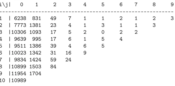
The incurred counts are shown in Table 2.
i\j| 0 1 2 3 4 5 6 7 8 9
---1 | 6238 831 49 7 1 1 2 1 2 3
2 | 7773 1381 23 4 1 3 1 1 3
3 |10306 1093 17 5 2 0 2 2
4 | 9639 995 17 6 1 5 4
5 | 9511 1386 39 4 6 5
6 |10023 1342 31 16 9 7 | 9834 1424 59 24 8 |10899 1503 84 9 |11954 1704 10 |10989
Table 2: The number of reported claims,Nij,(i, j)∈ A10, for the auto TPL.
For these data, as sometimes occurs in practice, some of the reported claims are settled with no payment. This can occur if, for example, there is consideration about who carries responsibility for a claim, fraud or similar. These are referred to as zero claims, and are, by nature, different from the claims which result in a payment. They can be dealt with in a number of different ways: for example, it would be possible to include in this set of claim numbers a separate class for those which are settled at zero. An alternative approach which leads to the same model is to use a claim severity distribution which is of mixed type. In this paper, we use the latter approach and use a claims severity distribution which a discrete probability that a claim is zero combined with a continuous claim size distribution. The probability that a claim is settled at zero is denoted byQ,
[image:13.595.151.455.341.490.2]distribution of claim payments is such thatP(Yij(k)= 0) = Qand the density ofYij(k)|Yij(k) >0 is denoted by f. The most natural assumption for f is that it is a Gamma distribution. However, for the purposes of this paper, we only consider the first two moments of this distribution. The expert advice from the company has been used to determine the fraction of reported zero-claims, , and the maximal possible RBNS delay,d≤10. In this case(Q, d) = (0.2,7).
Note that the mean and variance of the (non-zero) claim distribution,f, can be obtained from the estimates ofµandσ2, using:
µ=E[Yij(k)] = (1−Q)E[Yij(k)|Yij(k)>0]
and
σ2=V[Yij(k)] = (1−Q)V[Y
(k)
ij |Y
(k)
ij >0] +Q(1−Q)
E[Yij(k)|Y
(k)
ij >0]
2
.
Thus, the estimate ofE[Yij(k)|Yij(k)>0]is
Pd k=0ψkˆ
1−Q
and the estimate ofV[Yij(k)|Yij(k)>0]is
Pd
k=0ψkˆ
h
(1−Q) ˆφ−Pd
k=0ψkˆ
i
(1−Q)2
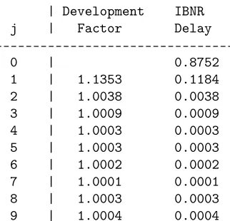
| Development IBNR
j | Factor Delay
---0 | 0.8752
1 | 1.1353 0.1184
2 | 1.0038 0.0038
3 | 1.0009 0.0009
4 | 1.0003 0.0003
5 | 1.0003 0.0003
6 | 1.0002 0.0002
7 | 1.0001 0.0001
8 | 1.0003 0.0003
9 | 1.0004 0.0004
Table 4: Development factors and distribution of the IBNR delay for the numbers of reported claims.
For the paid claim amounts the RBNS delay is given by the estimates of the parametersp0,p1,· · · , p7, which are shown in Table 5.
j | 0 1 2 3 4 5 6 7
---p | 0.3637 0.2881 0.1134 0.0852 0.0661 0.0358 0.0255 0.0222
Table 5: Maximum likelihood estimates ofpl,0≤l≤7.
Notice that IBNR delay (the last line in Table 4) and the IBNS delay (in Table 5) both sum to 1.
The estimates of the mean and variance of an individual (non-zero) claim severity are 203.01 and 3,496,125.
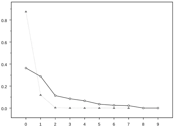
As was mentioned at the beginning of this section, the TPL claims are expected to have relatively long settlement delays (RBNS delays) as bodily injury claims often take a long time to settle, and this can seen from the left hand plot in Figure 1, since a long time after the majority of claims has been reported there are still some significant payments. Also notice thatp0 may be
relatively small. As claims happen, on average, in the middle of the year there is on average only half a year to receive the final payment in order to finish in the category of claims related top0. All other delay periods are full years.
Figure 1 compares the IBNR delay (from Table 4) with the RBNS delay (from Table 5).
0 1 2 3 4 5 6 7 8 9 0.0
[image:16.595.158.439.157.366.2]0.2 0.4 0.6 0.8
Figure 1: The dotted line represents the IBNR delay and the solid lines repre-sents the RBNS delay.
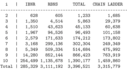
i | IBNR RBNS TOTAL CHAIN LADDER
---2 | 628 605 1,233 1,685
3 | 1,350 4,514 5,863 29,379
[image:17.595.133.399.123.269.2]4 | 1,510 43,623 45,133 60,638 5 | 1,967 94,526 96,493 101,158 6 | 2,579 171,633 174,212 173,802 7 | 3,168 299,136 302,304 249,349 8 | 5,349 509,334 514,684 475,992 9 | 14,280 852,144 866,423 763,919 10 | 254,499 1,135,678 1,390,177 1,459,860 Total | 285,329 3,111,192 3,396,521 3,315,779
Table 6: The row wise reserve estimates split into IBNR and RBNS claims, together with the chain ladder estimates
As discussed above, the IBNR delay is (on average) shorter than the RBNS delay, and hence the RBNS reserve is expected to be larger then the IBNR reserve. The actual estimates divide the reserves such that the RBNS reserve takes up91.6%of the total reserve and the IBNR only8.4%: roughly10 : 1 as suggested above. The chain ladder reserves include both the IBNR and a part of the RBNS claims, but it is not possible to split them.
7
Conclusion
This paper has developed a new stochastic model for claims reserving, which has a number of advantages over the standard approaches based on a single triangle of data (such as the chain ladder technique). A significant extra element in the results is that the sources of the delay in the claims process are split into the IBNR and RBNS components. We believe that this approach has the potential to make real improvements in the practical approaches to reserving, and the data study in Section 6 illustrates this.
The approach taken in this paper steers a middle course between the crude methods based on a single triangle and the very detailed methods based on data at the individual claim level. We believe that, in a practical context, this is a completely realistic approach: it does not throw away a lot of useful information, as the chain ladder technique does, but nor does it make very heavy extra computational demands.
References
Bühlmann, H., Schnieper, R. and Straub, E. (1980): Claims reserves in casualty insurance based on a probability model. Mitteilungen der Vereinigung Schweiz-erischer Versicherungsmathematiker.
England, P. D. and Verrall, R. J. (1999): Analytic and bootstrap estimates of prediction errors in claims reserving. Insurance: Mathematics and Economics, vol. 25, 281-293.
England, P. D. and Verrall, R. J. (2002): Stochstic claims reserving in gen-eral insurance (with discussion). British Actuarial Journal, vol. 8, 443-544
England, P. D. and Verrall, R. J. (2006): Predictive Distributions of Outstand-ing Liabilities in General Insurance. Annals of Actuarial Science, vol. 1, 221-270.
Hachemeister, C. A. and Standard, J. N. (1975): IBNR claims count estima-tion with static lag funcestima-tions. 12th Astin Colloquium, IAA, Portimao, Portugal.
Liu, H. and Verrall, R. (2009a): Predictive Distributions for Reserves which Separate True IBNR and IBNER Claims. Astin Bulletin, vol.39, 35-60.
Liu, H. and Verrall, R. (2009b): A Bootstrap Estimate of the Predictive Dis-tribution of Outstanding Claims for the Schnieper Model. To appear in Astin Bulletin.
Mack, T. (1991): A simple parametric model for rating automobile insurance or estimating IBNR claims reserves. Astin Bulletin, vol. 21, no. 1, 93-108.
McCullagh, P. and Nelder, J. A. (1989): Generalized Linear Models, second edition. Chapman&Hall, London.
Neuhaus, W. (2004): On the estimation of outstanding claims. Australian Actuarial Journal, vol. 10, 485-518.
Norberg, R., (1986): A contribution to modelling of IBNR claims. Scandi-navian Actuarial Journal, 155-203.
Norberg, R., (1993): Prediction of outstanding liabilities in non-life insurance. Astin Bulletin, vol. 23, no. 1, 95-115.
Norberg, R., (1999): Prediction of outstanding claims: Model variations and extensions. Astin Bulletin, vol. 29, no. 1, 5-25.
lia-bilities incorporating claim count uncertainty. North American Actuarial Jour-nal, vol. 6, no. 1, 113-137.
Renshaw, A. E. and Verrall, R. (1994): The stochastic model underlying the chain ladder technique. Actuarial research paper no. 63.
Schmidt, K. D. (2007): A bibliography on loss reserving.
Available on: http://www.math.tu-dresden.de/sto/schmidt/dsvm/reserve.pdf
Schnieper, R. (1991): Separating true IBNR and IBNER claims. Astin Bul-letin, vol. 21, 111-127.
Taylor, G.C. (1986): Claims reserving in non-life insurance. North Holland.
Taylor, G. C. and McGuire, G. (2004): Loss reserving with GLM - a case study. CAS discussion paper program, 327-391.
Verrall, R. J. (1990): Bayes and empirical Bayes estimates for the chains ladder. Astin Bulletin, vol. 20, 217-243.
Verrall, R. J. (1991): Chain ladder and maximum likelihood. Journal of the Institute of Actuaries, vol. 118, 489-499.
Verrall, R. J. and England, P. D. (2005): Incorporating expert opinion into a stochastic model for the chain-ladder technique. Insurance, Mathematic and Economics, vol. 37, 355-370 .
Wright, T. S. (1990): A stochastic method for claims reserving in general insur-ance. Journal of the Institute of Actuaries, vol. 117, 677-731.
Wüthrich, M.V. and Merz, M. (2008): Stochastic Claims Reserving Methods in Insurance. Wiley
Richard Verrall, Faculty of Actuarial Science and Insurance, Cass Business School, City University, London, [email protected]
Jens Perch Nielsen,Faculty of Actuarial Science and Insurance, Cass Business School, City University, London