The development and application of computer simulation models to biological systems

THE DEVELOPMENT AND APPLICATION OF COMPUTER

SIMULATION MODELS TO

BIOLOGICAL

SYSTEMS

by

John Stanley Armstrong

This thesis was submitted in partial fulfilment of the

requirements for the degree of

Master

of

Science

in

the

Australian National University

The work recorded in the thesis is my own except for the project concerned with the summer grazing model, where I was a member of a team. Here I acted initially as a consultant for Dr J.L. Davidson and Mr J.R.Donnelly, afterwards taking over the full responsibility for model design and development.

Acknowledgements List of Figures Summary

CONTENTS

Chapter l - Simulation

1.1 Introduction 1.2 A Definition

1.3 Problem Solving - Two Approaches

1.4 Analogue and Digital Computation

1.5 Interactive Computing

Chapter 2 - Comments on the use of Fortran and Simscript as simulation programming languages

2.1 Introduction 2.2 Model Struct ure

2.3 Storage Characteristics 2.4 Flowcharting

2.5 Communication

2.6 Technical Limitations 2.7 The Final Choice

Chapter 3 - Notes on Chapters 4, 5 and 6

Chapter 4 - Summer Grazing and Sheep Management Model

4.1 4.2

4.3

4.4

4

.

5

4.6

4

.7

4.8

4

.

9

Aim

Introduction and History Structure of the Model Events

Sets, Entities and Attributes Operation of the Model

Program Storage Requirements Output of Results

Future Development

Chapter 5 - Three-Dimensional Light Penetration Model

5.1 Aim

5.2 Introduction

5.3 General Description of

the Model

5.4 Operation of the Program

5.5 Simscript/Fortran Comparison 5.6 Program Storage Requirements

Chapter 6 - Two-Dimensional Light Penetration Model

6.1

6.2

6.3

6.4

6.5

6.6

6.7

6.8

6.9

Introduction

Leaf Representation General Model Structure Phase 1

Phase 2

Output Phase

Program St orage Requirements Visual Checks

Timing Considerations

Chapter 7 - Discussion and Conclusion 7.1 Introduction

7.2 General Approach

72 72 72 74 75 94

96

98 98 98 100 103 130 130 130 133 134 135 135

13

6

7.3 Interdisciplinary Group Action 138

References

Appendix 1

Appendix 2

7.4 Simulation Models as Research

Tools 140

7.5 Model Verification and

Dimensionality

7.6 Interactive Computing

Interactive Computing Facilit ies at

the Computing Laboratory, Division of Computing Research, CSIRO, ·Canberra

Flowchart for Consumeable Stores Inventory Simulation

142 143

146

150

Appendix 3 Simulation of Summer Grazing Appendix 4 Summer Grazing

Appendix 5 Vegetation-Environment Interactions

In Folder inside Back Cover

-Graph l

Graph 2

Interception of direct radiation. Plotter out put to check the program operation in Phase 1.

Interception of diffuse radiation. Plotter output to check the program operation in Phase 2.

153 163

ACKNOWLEDGEMENTS

I would like to express my thanks to Professor J.D. Ovington, Head of the Forestry Department, School

of General Studies, A.N.U., for permission to carry out this work, and to Dr L.T. Carron, Reader, Forestry

Department, for supervising the project.

The major part of the project involved working with a group in the Grassland Agronomy Section of t he CSIRO Division of Plant Industry, Canberra. In particular, I

have been associated with Dr M. Freer, Dr J.L. Davidson and J.R. Donnelly, and have appreciated their interest and cooperation.

The other part of the project involved members of the CSIRO Division of Land Research, Canberra. Thanks are due here to Dr

C.W.

Rose, Environmental Biology Group, for advice and for supplying many references. Professor R.O. Slatyer, Research School of Biological Sciences, Institute of Advanced Studies, A.N.U., gave considerable help in initiating t he project.

Mr R.E. Smart of the Viticultural Research Station, N.S.W. Department of Agriculture, suggested the

development of a two-dimensional model and supplied the

Figure

2.1

2

.

2

4.1

4.2

4.3

4.4

4.5

4.6

4.7

4

.

8

4.9

4.10

4

.

11

4

.

12

4

.

13

4.14

4

.

15

4.16

4.17

4

.

18

4

.

19

4

.

20

4.21

4.22

4.23

4.24

4.25

4.26

LIST OF FIGURES

Title

Timing and Space Requirements for GET and PUT Routines (Simscript )

Timing and Space Requirements for Instructions to Access or Restore Variables (Fortran)

Structure of Summer Grazing Model Flowchart showing interdependence of the events in the Summer Grazing Model Correspondence between the FARM and GRAS sets

Hierarchy of events dependent upon exogenous event START

Source listing for routine Source listing for routine Source listing for routine Source listing for rout ine Source listing for routine Source listing for routine Source listing for routine Source listing for routine Source listing for routine Source listing for rout ine Source listing for routine Source listing for routine Source listing for routine Source listing for routine Source list ing for routine Source listing for routine

START LOOK DSTRY AGIN CLEAN GRO EAT DECR GROFAT SAMPL DROUT MOVE SELECT TRMPL RAIN WETHR Graphs of dry mat erial on t he paddocks with time

Graphs of green material on the paddocks with time

Graphs of green material eaten from each paddock with time

Graphs of accumulated digest ible food units eaten with time

Graphs of sheep weight with time

Growth curves based on the equation by von Bert alanffy

Figure 4.27 4.28

5.1

5.2

5.3

5.4

5.5

5.6 5.7 5.8

5.9

5.10

5.11

5.12

5.13

5.14

5.15

6

.1

6.2 6.3

6

.4

6.5 6.6

6.7

6.8

Title Page

Curves of efficiency of eating with

amount of material available 68 Flowchart showing the general scheme

for interactive computing 71

Flowchart showing the general operation of the three-dimensional light

penetration model 76

Source listing for routine MAIN 77 VISTA Input/Output unit showing

messages on the screen, the light pen

and the keyboard 79

Flowchart for routine SETLUX 80 Source listing for routine SETLUX 81 Source listing for routine STRUCT 83 Display Console showing the file of

leaf values on the screen 85 Flowchart for routine TRACK 86 Source listing for routine TRACK

Source listing for routine ABSORB Source listing for routine ESCAPE Source listing for routine RFLECT Flowchart for routine RESULT

Source listing for routine RESULT Source listing of part of routine TRACK (Simscript )

Individual leaf profile Typical leaf structure

Flowchart showing the overall plan of the program

Typical situation in the model Flowchart of Phase l

Source listing for Phase 1 Flowchart for routine READDATA

Source listing for routine READDATA

Figure Title Page

6.9 Source listing for routine

MAXMIN

110

6.10 Source listing for routine PLOTLEAF 111

6.11 Diagram of overlapping by the leaves 112

6.12 Flowchart for routine

LAI

114

6.13 Source listing for routine

LAI

116 6.14 Flowchart for routine PDSORT 117

6.15 Source listing for routine PDSORT 118

6.16 Flowchart for routine CONTACT 120 6.17 Source listing for rout ine CONTACT 122

6.18 Diagram showing the interception of

diffuse radiation 123

6.19 Flowchart for routine DIFFUSE 125

6.20 Source listing for routine DIFFUSE 126 .21 Source listing for routine

BAMP

129

6.22 Flowchart of Phase 2 131

6.23 Source listing for Phase 2 132 In Holder, inside back cover

-Graph l

Graph 2

Interception of direct radiation. Plotter

output to check t he program operation in Phase 1. Interception of diffuse radiation. Plotter

SUMMARY

Biological systems are generally complex and the interrelations which describe the system response are

difficult to determine. Consequently, the construction of a model of such a system usually involves considerable abstraction. The recent advances in the computing field, notably in the speed of operation, storage space and

specialised simulation languages, do relieve some of the difficulty in making models of biological systems. The labour of numerical calculation is removed and a broader approach to the problem is possible. This thesis describes some work that has been done on three particular models.

The first is a model of a rotational sheep grazing system. It is written in Simscript and has been through several development phases. The present model is, to some extent, verified and it has been used for experimental

purposes.

The second and third models are concerned with light penetration into a leaf canopy. The second model considers the problem in terms of three-dimensional leaf

representation, with the energy distribution spectrum of the incident radiation represented by a number of wavebands. This model is in the prototype stage.

The third model is a simpler version of the second model. It uses a two-dimensional leaf representation. The approach and structure for this model are similar to that

initial design are satisfactory. Bot h these models are written in Fortran. Some comments on the two programming languages, Fortran and Simscript, are given.

Part of the work was to consider the use of the

interactive features now available on most medium to large scale computers. Previous engineering experience with analogue computers indicated the benefits that could be obtained by 'direct' manipulation of the model. The

provision of this kind of facility, enlarges the model t o include the experimenter, and the use of graphical output allows the experimenter to quickly get the 'feel' of the system under review.

That simulation methods have a place in the study of

biological systems is, by now, an historical fact. In the thesis, therefore, more emphasis is placed on the 'how' rather than the 'why' of simulation. Interactive computing

should feature prominently in the future application of

1.1 Introduction

l

SIMULATION

1

Agriculturists, engineers, economists and all whose discipline is based on the scientific method are familiar with the concept of a model. Models are on the same footing as hypotheses. They are attempts at description of a real system with an underlying purpose of understanding part, or all, of that system. As most systems are dynamic, models are usually concerned with the changes in system variables with time, due to external causes (i.e. changes which are imposed .on the system) or due to changes naturally occurring within the system.

1.2 A Definition

A good working definition of simulation is given by Shubik (1960). 'A simulation of a system or an organism is the operation of a model or simulator which is a

representation of the system or organisation. The model is amenable to manipulation, which would be impossible, too expensive or impractical to perform on the entity it portrays. The operation of the model can be studied and from it, properties concerning the behaviour of the actual system or its subsystems can be inferred'.

1.3 Problem Solving - Two Approaches

As examples of different approaches to problem solving, the fields of engineering and biology will be briefly

Engineering is, for the most part, the practical

application of simple well established theories in physics.

The difficulties in implementation are not directly due to

2

a lack of knowledge, but generally fall into two areas.

Firstly, there are economic, political, social and,

occasionally, even aesthetic constraint s. Secondly, while the theory may be well established, the application may lead to systems of equations,the solutions of which are beyond

the scope of contemporary methods. This second factor has

been largely removed by the advent of digital computers.

In earlier times, however, it was this difficulty that

induced engineers to develop the use of models. Scale models

of river systems, dam spillways, aerofoil sections and boat

keels are examples of attempts to short-cut the areas of

difficult calculation. A movement towards abst raction in models came with the mechanical differential analyser. On

this, a system of difference equations representing a dynamic

or rate controlled system could be set up. Following the

invention of amplifying valves, there was a natural

progression to electrical and electronic analogue computers.

These are used extensively for the analysis of such complex

systems as electric supply grids, in normal and fault

condition.

In biology the situation seems different While some

areas, such as genetics, are well defined by theory, for

many others no theory has evolved and an experimental

approach is favoured. In fact, the development of

statistical techniques has been strongly connected with the

programming have become the route by which biologists, and

others in the area of the natural sciences, have approached

biological problems. The construction of analytic

mathematical models of systems is common in research, for

example see Waggoner and Reifsnyder (1968), and Anderson and

Denmead (1969), but the use of analogue computers in this

context appears to be small.

3

For the engineer, the concept of a system with

interaction between its components is a familiar one. He is

used to dealing with them and accepts them as normal. He has

learned to predict the stability of systems and, where

necessary, to impose control over a system by the use of

negative feedback.

For the research biologist, the stability of natural

systems, coupled with their general complexity, makes

investigation of a whole system difficult, i f not impossible. Consequently, there is a bias towards looking at small parts of the whole which, when isolated, will not have all the

normal external influences affecting their behaviour.

Thus, the difference between the two disciplines is the

difference between a synthetic and an analytic approach.

It is interesting that the roles are changing over to

some extent. The engineer, physicist and economist are

finding situations where the past history of a system affects

its present response. This situation requires new methods of

analysis. Similarly, using the power of the digital computer,

and new techniques such as simulation, the biologist has the

opportunity to take a new look at the factors which determine

4

1.4 Analogue and Digital Computation

The main use of the electronic analogue computer is to model a system of linear or non-linear differential equations. It can be run with a one-to-one time correspondence with the actual system as in aircraft simulators, or at a faster or slower rote than real time. By this means, a physical

process which lasts only microseconds con be modelled in slow motion, and a process which lasts for days or years can be

'rushed' in a few seconds.

Practical advantages of the analogue computer ore that by using visual devices, such as cathode ray tubes, the

effects of parameter changes can be viewed immediately. The modular construction of the analogue computer makes it

amenable to quick modification. The main disadvantage is the lack of storage where results can be held and reviewed. In recent years, the basic electronic analogue computer has been extended by the addition of logic function and some storage. The more important development, however, is in the field of hybrid computation where a digital computer is

linked with an analogue computer. Each computer takes over that part of the task for which it is best fitted. In

general, this means the integration procedures are done by the operational amplifiers in the analogue computer (rather than by subroutines such as Runge-Kutta) and the logic, storage and general book-keeping are handled by the digital computer.

The development of special purpose simulation languages for digital computers has led to two distinct types evolving. The first type is designed to model systems in which the

5

variable, usually time. Exampl es are CSMP and COBLOC. The advantages of defining a model in these languages,instead of using an analogue computer directl~ are the elimination of scaling problems and of the necessity to carry out performance tests on each of the model components. A disadvantage is

that the user does not have immediate control over t he

system parameters. A limitation arising nat urally from t he use of a digital computer is that cont inuous variables must be represented by a discrete approximation, and integrat ion procedures will be comparatively slow. Where possible, t he combination of an analogue simulation language used for initial runs, followed by experiment at ion wit h t he model on an electronic analogue computer is a powerful approach.

The other type of simulation language arose in the first instance from work done on the simulation procedures required to process war and business games, invent ory

control, transportation problems and fact ory job scheduling. These processes are essentially discontinuous. The languages which result ed, such as GASP, CSL and SIMSCRIPT (all based on Fortran), SIMULA and ESP (based on Algol) and GPSS, each have areas of best performance, but each contains sufficient

generality to permit it to be applied to a range of problems. One of these languages, Simscript, has been used in

part of the work. In Chapter 2, the structure of this language and some comparisons with Fortran are made.

1.5 Interactive Computing

6

stimulating; in essence, it is the difference bet ween

driving a car and being driven. Following the recent advances in the input/output devices which can interface with a digital computer, on-line experimentation is possible in much the same way as with the analogue computer. The general arrangement is as follows:

-INPUT/ _{INTER- DIGITAL}

USER

-

OUTPUT _DEVICE

-

FACE

-

COMPUTER

The input/output device can be a t ypewrit er, or a display console with screen and keyboard (Fig. 5.7), or a television type screen with keyboard and facilit ies for input of information directly via the screen by a light

pen (Fig. 5.3). In order to make the process economic, the digital computer usually operates in time-shared mode, so that the computer is not idle when t he user is viewing the results, or changing system parameters.

Details of the interactive computing facilities which were used in the models are given in Appendix 1.

Kiviat (1967), an aut hority in this field, makes the following comment:

'Graphics and time-sharing also have a large future in simulation experimentation. While it is true that many simulation jobs are well structured and involve little more than substantial computer runs to estimate system

properties, a large number of people have jobs that are unstructured. They are interested in searching for

response surface. Batch-type processing hinders rather

than helps these jobs. A few minutes of console interaction with the right kind of displays can probably displace hours of conventional hit and miss experimentation. Little work

has been done on this aspect of interactive simulation. It seems like a very profitable area. '

2

COMMENTS ON THE USE OF FORTRAN AND SIMSCRIPT AS SIMULATION PROGRAMMING LANGUAGES.

2.1 Introduction

Fortran is a general purpose scientific programming language developed by

I.B.M.

It was introduced in 1958 and since then has been revised and enlarged. The version

considered here is Fortran IV.

8

Simscript is a special purpose programming l anguage designed for simulation problems. It was developed at the RAND Corporation and generally released in 1962. Since then, apart from improvements in the compilers, the

available versions are close to the original specifications. A new version called Simscript II, to be released shortly, is considerably more powerful and sophisticated than the version presently available. Details of Simscript II are given in an article by Kiviat (1966).

Whilst it is possible to consider Fortran as a virtual sub-set of Simscript, there are differences in language structure which tend to influence model construction.

Different models for the one problem would bear the peculiar characteristics of the language in which they are written.

2.2 Model Structure

For large programs written in Fortran, the strategy of using subroutines is normally adopted to achieve generality and flexibility. For example, in a forest inventory

called subroutines to read data referring to a sample plot, to check the data for range and other errors, to calculate increment statistics, to calculate volume statistics, to plot resulting curves etc. In subsequent uses of the program various subroutines could be omitted as required.

The transfer of information between the subroutines is normally by parameter lists but can also be done by defined common areas. This aspect will be mentioned again later.

9

Simscript, being initially designed as a special

purpose language, is more readily identified with the structure of the model it is used to define. In simple

terms, any model consists of things which are interconnected to form a system which,when subject to a stimulus, will

exhibit a characteristic response. In the Simscript language 'things' are defined as entities. The stimulus

and the effect it has on the entities is defined by an event

routine, which is broadly similar to the Fortran subroutine. The event routine is triggered not by a call as in Fortran

but by an event which can be initiated in one of two ways.

Either (1) os a statement in an event routine or (2) as an event card in the data. An event arising within an event

routine, which is known as an endogenous event, can refer

to another routine or it can be for the same routine in which it is situated. This is not in fact recursion but does enable an event to re-schedule itself automatically.

This is frequently useful where, for example, one may wish

In the flowcharts this type of event is shown

thus:-The circle, or part circle, implying re-scheduling and the

bar in the top right-hand corner indicating the process is

an endogenous event routine. The coding would look

something like this

-ENDOGENOUS EVENT EXAM

CAUSE EXAM AT TIME +DT

RETURN

END

xx

10

The statement xx will cause re-scheduling. After a time

period defined by DT the event routine will again be entered.

Events can be initiated for event routines other than

the parent routine and this situation is shown in the

flowcharts as below.

A

D

B

S/R

X

11

This would be interpreted

as:-Event routine A causes event routines Band D to occur. Event routine B causes event routine C and also calls

the subroutine X.

Internal (i.e. endogenous) events cannot, of course, be self starting so that the other type of event which is

defined in the data deck is considered to be an external, or exogenous, event. There must be at least one exogenous

event to start the simulation and the normal practice is to have a terminating exogenous event set for a particular time. Other exogenous events may or may not be required. Examples

of their use would be for external events such as buyers arriving at a supermarket, rainfall on a pasture system, or thinning in a forest. All of these could, of course, be defined as internal events if distribution functions are available which adequately describe the time and frequency of the events. For many models this kind of data is not available and, in any case, the externally defined events are amenable to change. In this way the user can experiment with 'typical', 'best' and 'worst' sequences for the

exogenous events.

On the flowcharts exogenous event routines are shown

12

2.3 Storage Characteristics

The state of a model written in Fortran will be expressed by the values of the various real and integer variables, subscripted or simple& In Simscript use is made of dynamic storage by list-processing and the notion of an array is replaced by a set, or list,which is composed of any number, including zero, of linked members. Thus, the state of the model in Simscript is represented by the state of the sets. In more detail the members of the sets, called entities, in turn hold one or more attribute values. To clarify this concept an analogy with Fortran is helpful, i f not pressed too far. One can think of a set as being comparable to a two-dimensional array, with a row in the array being equivalent to an entity, and a

particular element in the row equivalent to an attribute. To give a specific example - HUMAN could be an entity which might have the attributes WEIGHT, AGE, HEIGHT, COLOUR OF EYES and SEX. The last attribute SEX would be the determining factor for placing the entity into the set MALE or the set FEMALE.

For reasons of generality the creation of global variables by a COMMON statement in Fortran is not always favoured. The use of COMMON storage leads to faster

execution and saving in storage, as the interpretation of the parameter list and the space for the instructions to

perform this interpretation are eliminated. In Simscript, however, a basic feature is the list of the so called

~permanent attributes'. This is a common block and is

13

of an 'initial conditions deck' which in effect updat es the values of the permanent attribut es. One di fference from Fortran is t hat subscripted attributes can have variable dimensions without the necessity for ext ra coding and the use of EQUIVALENCE statements by the user. This is really an indication of the whole difference bet ween t he two

languages. Much of what can only be called book- keeping is automatically provided by the Simscript system, whereas in Fortran the user must take care of all aspects of the manipulation of the 'events' . For instance, with Simscript the main routine is provided by the system.

This background routine maintains an 'events list' in time order, and updates the list by adding new events or cancelling events as required. When a new entity is created the routine allocates the storage from the 'free' area and links t he new entity into its set. Should the free area become exhausted the program will undertake a 'garbage collection'. This involves the collection, for re-use, of entities which have been previously destroyed. All this is a considerable job and, for models with complex event-timing sequences, the provision of this main routine eases the

burden on the programmer. The light penetration and summer grazing models discussed in later chapters have a very

simple linear event structure, so the benefit is not so noticeable. In other models of industrial systems and in those where stochastic processes are involved, the

14

The use of the attribute-entity-set structure rather than subscripted variables is subject to compromise and the respective advantages depend strongly upon the model

considered. The most immediate benefit of Simscript is the close correspondence between the English description of the required action and the source statement . For example, i f the problem is to find the total weight of all men in a particular group over 40 years old, this could be done by two Simscript statements as

below:-LET WT

LET WT

= =

o.

WT+ WEIGHT (HUMAN), FOR ALL HUMAN IN MALE, WITH AGE (HUMAN) GR 40.

Another obvious advantage is with list-processing there is no need to specify beforehand the storage requirements as in the Fortran DIMENSION statement.

The major drawback is that access to an attribute value

in a particular entity is much slower than to an element in an array. This is because it is necessary to ~link along' the entity chain until the correct entity is reached. Thus the access time is variable and can be high when long lists are used. In the summer grazing program the execution time for the simulation from day 1 to day 100 varied between 20 and 45 seconds depending upon the input parameters, the main variation being due to the selection of a one or nine paddock rotation. A similar prugram in Fortran required about ten seconds for the single paddock case. The

15

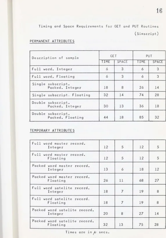
associated with it 'GET' and 'PUT' routines. These are all part of the book-keeping. The 'GET' routine for instance extracts that part of the entity record which contains the attribute in question. Similarly, the ' PUT' routine

implants the new value of the attribute. These routines can be as small as three or as long as 32 computer words, the range depending upon two factors. The first is the structure of the entity which may be simple, being a one, two, four or eight word record, or complex when there are up to eight sub-records linked to a master record. The second factor is the packing of attributes in a word. There can be one, two, three or four attributes per word. So that, besides the increase in access time already mentioned due to the list structure, there is a further penalty in time which will vary with the entity structure. To confound the picture further, where the attributes are in floating point format and are packed two or three to the word they will also require routines to unpack the exponent and fractional parts before being used in calculation.

The tables in Fig. 2.1 give some examples of the

average execution time and storage required for a sample of the 'GET' and 'PUT' routines.

16

Timing and Space Requirements for GET and PUT Routines (Simscript) PERMANENT ATTRIBUTES

Description of sample GET

TIME SPACE

Full word. Integer 6 3

Full word. Floating 6 3

Single subscript.

Packed. Integer 18 8

Single subscript~ Floating 32 14 Double subscript.

Packed. Integer 30 13

Double subscript.

Packed. Floating 44 18

TEMPORARY ATTRIBUTES

Full word master record.

Integer 12 5

Full word master record.

Floating 12 5

Packed word master record.

Integer 13 6

Packed word master record.

Floating 26 11

Full word satelite record.

Integer 18 7

Full word satelite recordo

Floating 18 7

Packed word satelite record.

Integer 20 8

Packed word satelite record.

Floating 32 13

Times are in

jJ

secs.

Space is in 48 bit words.

PUT

TIME SPACE

6 3

6 3

26 14

74 28

36 18

85 32

12 5

12 5

18 12

68 27

19 8

19 8

27 14

75 28

[image:27.661.35.606.29.850.2]

17

As a comparison, the execution times and storage space

requirements in Fortran are shown in Fig. 2.2.

Timing and Space Requirements for Instructions

to Access or Restore Variables

(Fortran)

DESCRIPTION TIME SPACE

Simple variable

4.0

1.0

Single subscripted variable

6.5

1.5

Double subscripted variable

6

~

5

3

o

5

Triple subscripted variable

6.5

4.5

Times are in~ sec.

Space is in 48 bit wordso

The time values are the result of a short test program

in which the array elements were accessed and restored

several million times~ The time equivalence in the single,

double and triple subscripted variables is surprising~

The machine language coding produced by the compiler

indicates the storage area required for the subscript

transformation but does not show the contents of the area.

It should be eriiphasised that the ability to pack more

than one numerical or alphanumerical variable (attribute)

into a word is an option which in terms of storage might

18

With Simscript, or for that matter Fortran or any other

high level language, efficient coding demands more than a

superficial knowledge of the language.

2.4 Flowcharting

A general difficulty with the documentation of computer

based models is to give a meaningful flowchart description

for the overall action. Flowcharts of finite programs have

an inbuilt dynamic character since they must show the

progression within the logical bounds which constitute the

solution to the initial problem. Where the problem itself

has a dynamic property, and particularly where stochastic

processes are involved, representation is difficult. The

solution adopted by the author is to present the flowcharts

at two levels, one to show the gross relationships between

the dynamic components of the model and the other to

indicate the detailed structure of each component. This

detailed level of flowcharting within the event routine,

function,or subroutine, is little different from traditional

flowcharting used to describe Fortran programs. Examples

are given in Chapters 4,5 and 6.

At the more abstracted level, the interconnection

between event routines, functions and subroutines is shown

with the dynamic sense implied by arrows on the flow lines.

For an example of such a flowchart see Appendix 2. This was

drawn by the author for a seminar given by Mr I. Ridgway.

It represents the structure of a consumeable stores

inventory simulation.

19

this is sometimes shown explicitly for information purposes, though of course every event has access to all sets in the simulation.

In other situations,more emphasis is placed on the sets and they become the main items in the flowchart with the various routines which affect the sets shown linked to them. This also seems to be a worthwhile approach since it is the current membership of the sets and their attribute values which define t he st atus of t he system. A further

advantage is that such flowcharts, designed to the

requirements of the professional programme~ can be re-drawn to convey the basic concepts in the model to a lay audience. This has been done in the flowcharts for the summer grazing

simulation. One of the two papers on this model was

prepared for a conference of computer simulation experts and the other for a congress where the main emphasis was on

application rather than methods and the average member of the audience would not be familiar with flowcharting. See Fig. l of Appendices 3 and 4.

2.5 Communication

As already hinted, Simscript, like Algol, is a better communication language than Fortran and for many of the

smaller routines a flowchart is not necessary. Against this some of the cryptic statements in Simscript can be confusing, for

example:-CREATE DOG CALLED FIDO

may seem reasonable, but

CREATE DOG CALLED DOG

[image:30.653.41.625.23.867.2]

after 'CREATE' does not have the same meaning as 'DOG' after 'CALLED'. Then to be told that the phrase 'CALLED DOG' can, in this case, be omitted anyway as redundant is enough to

baffle anyone. The point is computer programs currently require a high order of specificity for efficient compiling, and this in turn demands a level of understanding by the user.

2.6 Technical Limitations

One lesson which is quickly learned is that the

detection and location of errors (debugging) increases in difficulty with the level of the language. Simple

typographical errors are of no concern but with the higher level languages such as Simscript, where there is much more freedom of expression, many errors which are logically

executable pass undetected and require careful analysis to detect. The latest versions of Simscript promise better diagnostic facilities, but the fact remains one is dealing with a powerful weapon and care is required. In Australia few people are fully conversant with Simscript and advice is not readily available. Fortran on the other hand is widely used and expert advice is readily available. Related to this is the fact that not all computers have Simscript compilers, though this situation will change markedly over the next five years.

21

Re-compilation of a subsection of a Simscript program is possible but the complex nature of the compilation process, compared to that for Fortran, means two or three minutes are usually required. Most computer centres schedule incoming

jobs in terms of total time required for the job and/or storage requirements. Since the ' t urn-around' time for a

job is a highly non-linear function of the job time, the development stages of a project can be seriously hindered by high compilation times. The availability of fast Fortran compilers, such as

KWICTRAN,

together with on-line editing facilities speeds the development of Fortran based programs. For example, the program for the two-dimensional model took 27 seconds to compile under KWICTRAN and 93 seconds under Fortran. For these practical reasons, the original Simscript version of the three-dimensional model was rewritten in

Fortran.

2.7 The Final Choice

There is no easy solution to the questi on of choice between the languages. In some cases due to storage considerations, computers available, or a lack of expert advice, there will be no choice anyway. Timing comparisons between similar programs in different languages are difficult

to interpret. It is rather like comparing two different means of transport, say a car and an aeroplane - both may be able to get you from A to B but until you define exactly

and Lubin (1966), Tocher (1965), Brennan and Linebarger

(1964) and Krasnow and Merikallio (1963).

22

To conclude, it is t he author's opinion that for models

where there are no difficulties due to storage limitation,

and the 'cause and effect' mechanisms are reasonably simple,

FORTRAN (or ALGOL) i s the best choice. If the user wishes

to program in 'Simscript style' but remain within Fortran,

the GASP package of Fortran routines is suitable. For the

complex model with storage problems, Simscript is the most

23

3

NOTES ON CHAPTERS 4, 5 AND 6

The three models to be considered

are:-(1) Summer Grazing and Sheep Management.

(2) Penetration of Sunlight into a Canopy considered as a three-dimensional problem.

(3) As (2) but considered as a two-dimensional problem.

They are described in Chapters 4, 5 and 6 with a slightly different approach in each case. For the summer grazing model a full description of the history, model structure,and operation has been given. In this way the power and convenience of the Simscript language will be apparent,and the points made in Chapter 2 can be related. Comments are also made on the program storage requirements and on current development of this model. The application of the model is only mentioned in the chapter but is covered in the two papers, Appendices 3 and 4. These should be read in conjunction with Chapter 4.

The light penetration model for t hree dimensions is used as a vehicle to illustrate the structure of a model which is designed for on-line simulation experiments. In this case the model description and program operation has been

contracted somewhat. As this model is still in the prototype stage there are no results for comparison with field and

24

The third model is also concerned with light penetration and as the model design is very similar to that for the three dimensions model the structure, operation, and programming details are given a full treatment. The value of visual output for checking purposes is shown.

In all three chapters,subprograms in the models are

described by the text, by flowchart, by source listing, or by a combination of these. The text outlines the action of the subprogram. Comments in the source listing define the

infra-structure. Flowcharts are used at various levels of complexity, as appropriate. The source listings have been edited from the originals to exclude all details not directly involved in the model. All FORMAT, COMMON, DIMENSION and non-executable statements of this t ype have been removed together with calls to various checking routines, optional printing statements and timing calculations. Most of the error messages have been replaced by single line comments and some of the input/output statements have been simplified.

The method of producing the source listings is

interesting. Instead of taking photocopies of the direct computer listing, the source deck was translated into paper tape form and this was used to drive a typewriter. The characters are generally clearer than those in the

25

4

SUMMER GRAZING AND SHEEP MANAGEMENT MODEL

4.1 Aim

The aim was to construct a model which in a realistic

and reasonably accurate manner presented the structure and

interactions which occur in a system of sheep management.

4.2 Introduction and History

In normal practice a flock of sheep are rotated between

paddocks where they have access to two types of grass; green

(i.e. living) and dry (dead). Rainfall produces green grass

of a given digestibility. This green material will decrease

in digestibility with time until after a set period it is

considered to be dead and is reclassified as dry material.

Both green and dry grass will be reduced by being eaten by

the sheep and the dry material is also reduced by three

other actions. These are weathering losses following rain,

trampling losses due to the sheep,and a time loss,

presumably due to wind and insects, which is found to occur

in the absence of both rain and animals.

Figure 4.1, taken from the paper 'Simulation of Summer

Grazing' (see Appendix 3), shows the structure of the present

model. For example, the green material is either eaten, is

added to the dry material after aging or remains green.

Having described in general terms the elements in the

model, it will be useful to give a brief history of the

[image:36.666.34.640.67.861.2]

26

The initial study was done by two groups in the

Grassland Agronomy Section of the Division of Plant Industry, CSIRO, Canberra, following a course on the simulation

language Simscript which the author gave at the Division of Computing Research, CSIRO. One group used Simscript and the other Fortran and the model was limited to consideration of dry material only. The results from the t rial study were encouraging and it was decided to increase the scope and realism of the model by introducing green material along with other changes. This was done and the model steadily developed. Areas of weakness in the model, mainly in the estimation of dry material losses, and where the data was insufficient, were reviewed and a series of field experiments arranged.

Further development of the model is proposed. This will be discussed after the following description of the present model .

4.3 Structure of the Model

The general structure of the model, indicating the

supply and demand on the green and dry material, is shown in Fig. 4.1, taken from Appendix 3.

In the more detailed Fig. 4.2, from Appendix 4, the connection is shown between the event routines, subroutines and sets of entities. The full lines with the single arrow indicate that an event, or events, are scheduled by the present event. For example, the event

RAIN

will cause the event WETHR to occur subsequently. The full lines with

[image:37.667.43.649.24.864.2]

Green material

Soil moisture

Evaporation

Dry mat erial

Weathering loss

Rai n

Time l oss

St ructure of Summer Grazing Model.

Trampling

loss

Fig. 4.1

Herbage eaten

START

_LOOK

~

SAMPL

~

..

L

DROUT

SELECT~

MOVE

_I /

/

I /

'

/

I

/

'

'

[:]

/ /

.

_

DRY

--

_..

/

-

...

-

-

_,...

_:

DISTRY

k

I

_WETHR

_I

_TRMPL

I

~

EAT

,,

I

RAIN

l

~

DECR

-;--;

,,,,, ,,,., I

GRO

I

(

GROFAT

~

--AGIN

r

- ....

-1

GREEN

t

---Flowchart showing the interdependence of the _{events in the Summer Grazing Model.}

Fig. 4.2

29

variables which are altered in one routine will affect t he

calculations in another. This is not unusual but , as

mentioned in Chapter 2, global variables (i.e. the permanent

attributes) and the sets are available to all routines and

an explicit indication of the part i cular connection between

routines is helpful in representing the structure and interactions.

4.4 Events

There are three externally applied or exogenous events,

START, RAIN and SIMEND (not shown in flowchart), and eleven

internal or endogenous events, AGIN, CLEAN (not shown in

flowchart), DROUT, DSTRY, EAT, GRO, LOOK, MOVE, SAMPLE,

TRMPL and WETHR.

4.5 Sets, Entities and Attributes

The emphasis in the model is on the pasture and its

variation during a grazing period of nominally 100 days.

The green material is represented by entities called GREEN

which are members of the set GRAS. This set is subscripted

such that the number of GRAS sets is equal to the number of

paddocks available to the sheep. The attributes of the

REF Paddock Identification l to NP where there

are NP paddocks

AGE Age of the green material in days. This

attribute is used to rank the set

GRE

DIG

SHNO

PRGE

GRUET

GREET

PGRASS

SGRASS

l

Amount of green material

Digestibility of the green material

Number of sheep on this paddock

Proportion of green eaten

Green units eaten

Green eaten

Attributes necessary for the automatic linking

of the member entities to form the set

30

The other entity in the model is not DRY as in the

flowchart but PDK which holds other information besides the

dry material. There is one PDK entity for each paddock and

The attributes of PDK are as

follows:-SFARM

REF

AMT

DIGAV

GRN

Attribute for list linking

Paddock identification l to NP where there

are NP paddocks

Amount of dry material

Average digestibility of the dry material

Total green material on the paddock

31

THDE

THI

PGE

Digestibility per cent of the dry material eaten

THIG

THAE

TTDUE

ADST

DULT

AW

TDUA

DULW

Theoretical intake of dry plus green

Proportion of green in the diet

Theoretical intake of green material

Theoretical intake of dry material

Digestible units of dry eaten

4mount of dry lost by time

Digestible units lost by time

Amount of dry lost by weathering

Amount of digestible dry available

Digestible units lost by weathering

Some of the attributes are common to the two entities.

The correspondence between the two types of set is

Paddock 1 Paddock 2 _{Paddock 3}

,---

- -

-

- -

-

- - -

-,

FARM f

G;J

_~

_~

I

I

...L.._

- -

_{- - - -- - - - -} _ 1 _

, - -

-I

,- ---1

,---

-r

1

~

1

_l

_~

_I

,

~

,

I

_I

I

I

I

I

~

~

I

~

I

I

I

I

_I

_I

I

~

~

_I

G;;]

I

_I

~ ~

I

~

I

~

₈

_~

I

l

~AS

(!)

GRAS (2) GRAS (3)

-

- - - _-

-Correspondence between the FARM and GRAS sets.

Fig. 4.3

The set FARM will always exist with NP entities where NP is the number of paddocks in the model. The GRAS sets will be zero member sets until the event of RAIN when the growth of grass results in the creation of GREEN entities.

[image:43.670.39.658.25.829.2]

33

4.6 Operation of the Model

Whilst the complete structure is shown in Fig. 4.2,

it is too complicated for looking at the program operation.

The operation will be described in the way it occurs in

practice, i.e. each external event, in order of occurrence,

and the internal events dependent on it.

In general, the events and routines have a simple

internal structure and flowcharts are not given. A number

of comments have been placed in the listings to explain the

general purpose and to indicate main points.

The first event is START. Its hierarchy of dependent

events is shown in Fig. 4.4.

is Fig. 4.5.

The source listing for START

As explained in the listing, START reads in the basic

paddock data and schedules further internal events. The

major one of these is LOOK. This routine effectively

controls the simulation as it is responsible for scheduling

the other important events concerned with the growth of new

grass (GRO), the reduction due to eating (EAT), and the

checking event (SAMPL), which manages the movement between

paddocks (MOVE) or into drought yards (DROUT) . The source

listing for LOOK is Fig. 4.6.

Where the scheduling of events is conditional on some

calculated limit, flags are set or reset as appropriate to

skip over sections of the routines. For example, in LOOK

i f there has been no rain, variable A which represents the

potential growth of green material will be zero and so the

event GRO will not be scheduled. Similarly, FLAGG will be

zero if the potential growth has been realised and again

START

LOOK

DSTRY

AGIN

CLEAN

DECR

GRO

EAT

SAMPL

TRMPL

GROFAT

MOVE

DROUT

SELECT

Hierarchy of events dependent upon exogenous event

START

Fig. 4.4

[image:45.669.60.657.21.855.2]

FIG.

4

.

5

SOURCE LISTING FOR ROUTINE START

EXOGENOUS EVENT START

C THIS ROUTINE STARTS THE SIMULATION RUN

C IT INITIALIZES THE PADDOCK DATA FROM DATA CARDS,

C ALLOCATES THE SHEEP TO THE FIRST PADDOCK ANO C SCHEDULES THE EVENTS LOOK, DSTRY, AGIN ANO CLEAN

C

LET ANP

=

NP

C MIXED MOOE EXPRESSIONS NOT ALLOWED LET FSIZE

=

FSIZE * ANP

C EACH PADDOCK IS NOMINALLY ONE HECTARE. FSIZE IS THE C STOCKING RATE SO THAT THE ACTUAL NUMBER OF SHEEP IS

C DIRECTLY PROPORTIONAL TO THE NUMBER OF PADDOCKS (NP)

DO , FOR J = (

1 )

(NP)

CREATE POK CALLEO K

C READ IN THE INITIAL AMOUNT OF DRY MATERIAL C ANO ITS DIGESTIBILITY

READ , AMT(K) , DIGAV(K) LET REF(K)

=

J

I F J E Q

1

,

LET SH NO ( K )

=

F S I Z E

IF J NE

1

,

LET SHNO(K) =

0.0

FILE K IN FARM

LOOP

CREATE LOOK

C SCHEDULE EVENT LOOK

CAUSE LOOK AT TIME+

0.1

CREATE DSTRY

C SCHEDULE EVENT DSTRY

CAUSE DSTRY AT TIME+

0.2

CREATE AGIN

C SCHEDULE EVENT AGIN

CAUSE AGIN AT TIME+

1.0

CREATE CLEAN

C SCHEDULE EVENT CLEAN

CAUSE CLEAN AT TIME+

1.1

RETURN ENO

FIG.

4.

6

SOURCE LISTING FOR ROUTINE LOOK

ENDOGENOUS EVENT LOOK

C TH IS ROUTINE IS SCHEDULED INITIALLY BY START C ANO SUBSEQUENTLY BY ITSELF

C IT SCHEDULES GRO, EAT, SAMPL ANO TRMPL C C C C C C C C C C C C C C

ER IS THE RATIO OF ACTUAL TO TANK EVAPORAT ION LET ER= GL*(1 .0 - EXPF(- GK*SM))

SM IS THE AVAILABLE SOIL MOISTURE LET SM= SM+ RFALL - ER*EVAP

IF THERE IS NO POTENTIAL GROWTH OR GROWING HAS STOPPED DO NOT SHEOULE GROWTH

IF A EQ 0.0 GO

1

IF FLAGG EQ

O

,

GO 1 CREATE GRO

CAUSE GROAT TIME

IF DROUGHT EXISTS OMIT EAT SECTION (SHEEP ARE HANO FED IN YARDS IN THIS CASE)

1 IF FLA GO EQ 1 , GO

2

FINO FIRST , FOR ALL KK IN FARM , * WITH SHNO(KK) NE 0.0 , WHERE K FIND WHICH PADDOCK HAS THE SHEEP

DEPENDING ON THE AMOUNT ANO THE PREVIOUS PROPORTION OF GREEN MATERIAL EATEN SHEDULE EITHER 1 OR 10 EATS

FOR THE NEXT DAY TOGETHER WITH A CORRESPONDING NUMBER

OF SAMPLING EVENTS

IF GRN(K) LS GM, GO

4

IF PGE(K) LE PGM , GO

4

J

LET FLAGE = 1.0

CREATE EAT

CAUSE EAT AT TIME CREATE SAMPL

CAUSE SAMPL AT TIME+ 0.8

GO

5

4

LE T FLA GE = 1 0 • LET TTT = 0.0

DO , FOR NE =( 1 ) ( 10) CREATE EAT

CAUSE EAT AT TIME+ TTT CREATE SAMPL

CAUSE SAMPL AT TIME+ TTT LET TTT = TTT + 0.1

LOOP

SCHEDULE THE TRAMPLING EVENT

5

CREATE TRMPL

CAUSE TRMPL AT TIME LET TYME = TYME + 1

RE- SCHEDULE LOOK

6

CAUSE LOOK AT TIME+ 1.0

CALL RECD

RETURN

2

CREATE SAMPL

CAUSE SAMPL AT TIME+ 0.8

GO

6

RETURN

ENO

[image:47.676.40.659.42.868.2]

37

The events DSTRY, AGIN and CLEAN are ini tiated by START and subsequently ore self sustaining.

DSTRY, Fig. 4.7, defines the loss in dry material with time? The loss is assumed to be a function of t he

digestibility of the material, such t hat the digestibility of the material lost is higher than the average

digestibility. This is a similar effect to the selection of dry material by the sheep, considered later, and t he same routine DECR is used to est ablish t he di gestibility of t he dry material lost .

FIG.

4

.

7

SOURCE LISTING FOR ROUTINE DSTRY

C

C C

C

C

C C

C C

C

ENDOGENOUS EVENT DSTRY

THIS ROUTINE IS SCHEDULED INITIALLY BY START AND SUBSEQUENTLY BY ITSELF

CALCULATION OF DRY MATERIAL LOST WITH TIME

SET FLAG SO ALL PADDOCKS ARE CONSIDERED IN DECR

LET FLAGS=

0

CALL DECR

AMOUNT LOST IS EQUAL TO THE AMOUNT PRESENT TIMES

THE RATE OF LOSS

LET ADST(K) = AMT(K) *OSK, FOR ALL K IN FARM

DIGESTIBLE UNITS LOST IS THE AMOUNT LOST TIMES THE DIGESTIBILITY SELECTED

LET DULT(K) = ADST(K)*THDE(K), FOR ALL K IN FARM RE- SCHEDULE THE EVENT

CAUSE DSTRY AT TIME+

1.

0

3

8

AGIN, Fig. 4.8, processes the GRAS sets . It updates the

age and digestibility attributes for each entit½ and updates the total green material available attribute which is in the

corresponding paddock. For the purposes of the model green material over a certain age is considered to have died. Any

which meet this criterion are removed from the GRAS set and added to the dry material attribute in the paddock, with a corresponding adjustment to the average digestibility of the dry material.

CLEAN, Fig. 4.9, is a programming convenience. It

happens that when the potential growth has been realised for a paddock,the GREEN entity, which is created to hold the amount of green material grown, has in fact a zero amount of

green. In order to keep the GRAS sets as small os possible and so reduce the time to process them, every three days the

non-useful entities are removed and the storage released.

FIG.

4

.

9

SOURCE LISTING FOR ROUTINE CLEAN

C C C C C C C

ENDOGENOUS EVENT CLEAN

THIS ROUT INE IS SCHEDULED INITIALLY BY START ANO SUBSEQUENTLY BY ITSELF

ANY ATTRIBUTE WHOSE GREEN ATTRIBUTE IS ZERO

IS REMOVED FROM THE GRAS SET

RE-SCHEDULE THE EVENT

CAUSE CLEAN AT TIME+

J

.

0

DO , FOR J

=

(1)(NP)

IF GRAS(J) IS EMPTY, GO 1

00 , FOR ALL G IN GRAS(J)

IF GRE(G) NE

(0.),

GO

2

REMOVE G FROM GRAS(J) DESTROY GREEN CALLED G

2

LOOP

FIG.

4.8

SOURCE LISTING FOR ROUTINE AGIN

ENDOGENOUS EVENT AGIN

C THIS ROUTINE IS SCHEDULED INITIALLY BY START C AND SUBSEQUENTLY BY ITSELF

C C C C C C C C C C C C C C C C

THE AGE AND DIGESTIBILITY ATTRIBUTES IN THE GREEN ENTITIES ARE UPDATED. ANY DEAD MATERIAL (AGE= AMX)

IS TRANSFERED TO THE POK ENTITY ANO THE NEW VALUE OF DIGAV IS CALCULATED

RE-SCHEDULE THE EVENT

CAUSE AGIN AT TIME+ 1.0 DO , FOR J = (1)(NP) REMOVE FIRST K FROM FARM

IF NO MEMBERS IN THE SET OMIT CALCULATION IF GRAS(J) IS EMPTY, GO

2

INCREASE AGE ATTRIBUTE BY 1 DAY

LET AGE(G) = AGE(G) + 1. , FOR ALL G IN DECREASE DIGESTIBILITY ATTRIBUTE BY AMOUNT LET DIG(G) = DIG(G) - AG, FOR ALL G IN FINO TOTAL AMOUNT OF GREEN IN THE SET ANO TRANSFER RESULT TO THE PADDOCK

GRAS(J) AG

GRAS(J)

LET SGRE(J) = 0.0

LET SGRE(J) = SGRE(J) + GRE(G), FOR ALL G * IN GRAS(J), WITH AGE(G) LS AMX

LET GRN(K) = SGRE(J)

CHECK IF ANY GREEN HAS AGE EQUAL TO AMX

IF SO ADO TO DRY IN PADDOCK ADJUST THE AVERAGE DIGESTIBILITY ANO FREE THE STORAGE TAKEN UP BY THAT GREEN ENTITY

FINO FIRST, FOR ALL G IN GRASS(J), WITH AGE(G) * EQ AMXJ WHERE NJ IF NONE

1 GO

2

LET AMT~K) = AMTlK) + GRE~N)

LET DIGAV(K) = (OIGAV(K)*AMT(K) + DIG(N)*GRE(N)) * /(AMT(K) + GRE(N))

REMOVE N FROM GRAS(J) DESTROY GREEN CALLEO N

2

FILE K IN FARM

LOOP RETURN ENO

4

0

The event GRO, Fig. 4.10, defines the daily growth of green material for each of the paddocks. A logistics growth curve is used with an initial step response following the first rainfall. This has not been completely satisfactory and further comments are reserved for a later section.

It is in GRO that the non-useful GREEN entities can be formed as noted earlier in CLEAN. Only when all paddocks have achieved their potential growth will the growth flag be reset.

The event EAT, Fig. 4.11, is scheduled by LOOK and can occur either once or ten times each day. The requirement to schedule ten EATS only occurs when the amount of green

material is small as in this case the function defining the amount removed by the sheep to the amount available is

convex and the change in gradient is comparatively rapid for small changes in amount available. With the coarse grid, i.e. one EAT per day, it is possible by extrapolation to remove more green than is currently available.

As eating only occurs on one paddock, the subroutine DECR, Fig. 4.12, is called with FLAGS set to unity. This routine establishes the proportion of green in

the diet available on the paddock and the theoretical intake of the total food and similar statistics for the green and dry materials.