A co-operating solver approach to building simulation

A CO-OPERATING SOLVER APPROACH TO BUILDING SIMULATION

Clarke J A and Tang D

ESRU, University of Strathclyde

[email protected]

ABSTRACT

This paper describes the co-operating solver approach to building simulation as encapsulated within the ESP-r system. Possible adaptations are then considered to accommodate new functional requirements.

Ke ywords: Building performance, integrated

mod-elling, equation solution, future requirements.

INTRODUCTION

There are three drivers for the growing uptake of integrated building simulation: the issues underly-ing sustainable development are too complex to be addressed by simplified design tools; simula-tion, where well applied, can lead to reduced design times and costs; and future legislation will call for integrated modelling in practice (e.g. the European Commission’s Energy Performance of Buildings Directive).

Further, it may be expected that the demand for integrated modelling will continue to grow as appraisals of life cycle performance and impact become the norm. This will place new burdens on the methods that are presently used to solve the underlying mathematical models.

This paper details the co-operating solution methods presently employed within ESP-r to solve the conservation equations relating to the interacting technical domains: building thermal processes, inter-zone air flow, intra-zone air movement, HVAC systems and electrical power flow. Options for solver adaptation are then dis-cussed as required to support the ’deepening’ of the domain treatments to include issues such as occupant interaction and embedded renewables.

INTEGRATED SIMULATION

Within ESP-r (Clarke 2001) a building comprises a collection of interacting technical domains, each solved by exploiting the specific nature of the underlying physical and mathematical theories (linear/non-linear, sparse/compact,etc). Examples of important couplings include: building thermal processes and natural illuminance distribution; building/plant thermal processes and distributed fluid flow; building thermal processes and intra-room air movement; building distributed air flow

and intra-room air movement; electrical demand and embedded power systems (renewable energy based or otherwise); and construction heat and moisture flow. This section describes the core domains of building thermal, inter-zone air flow, intra-zone air movement, HVAC systems and electrical power flow in terms of the approach taken to solve the describing equations while pre-serving essential domain interactions.

Building thermal processes

The conductive, convective and radiative

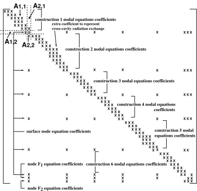
exchanges associated with the building construc-tions are established as a set of energy balance equations and a direct solution method applied. The approach is based on a semi-implicit scheme, which is second-order time accurate, uncondition-ally stable for all space and time steps and allows time dependent and/or state variable dependent boundary conditions and coefficients. Iteration is employed for the case of non-linearity where sys-tem parameters (e.g. heat transfer coefficients) depend on state variables (e.g. temperature). An optimised numerical technique is employed to solve the system equations simultaneously, while keeping the required computation to a minimum. As an example, consider the energy balance equa-tion-set for a simple room when expressed in matrix notation:

Aθn+1=Bθn+C

where A and B are coefficients matrices

corre-sponding to the future (n+1) and present (n) time rows respectively,θ a vector of node temperatures

and flux injections andCa known boundary

con-ditions vector. Since all parameters on the right hand side are known, the equation simplifies to Aθn+1 _=Dn

. The content ofA(from Clarke 2001)

is shown in Figure 1 for a 6-sided room with uni-directional conduction and a single air node.

The top left corner sub-matrix corresponds to the wall 1 internal nodes, while the sub-matrix (single equation) immediately below on the diag-onal corresponds to the wall 1 surface node. Simi-larly, there are sub-matrices corresponding to con-structions 2 through 6. The last coefficient on the

diagonal ofAcorresponds to the air node within

node F2 equation coefficients node F1 equation coefficients surface node equation coefficients

construction 1 nodal equations coefficients

construction 2 nodal equations coefficients

construction 3 nodal equations coefficients

construction 4 nodal equations coefficients

construction 5 nodal equations coefficients

construction 6 nodal equations coefficients extra coefficient to represent

cross-cavity radiation exchange

A1,1

A2,2

A2,1

A1,2

Figure 1: The future time row matrix,A.

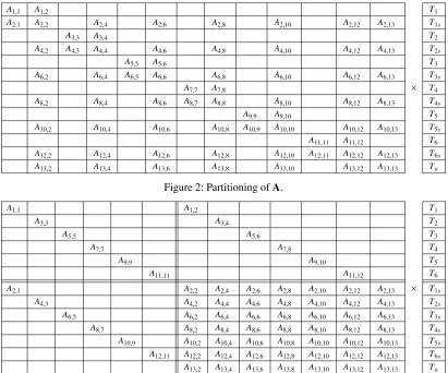
Such a system of equations can be solved effi-ciently by partitioning and reordering: Figure 2 shows the outcome when applied to the coeffi-cient matrix of Figure 1. Note that null matrices are not shown; sub-matrices in the even rows and the last row are single equations; andTi,Tis and

Ta correspond to the temperatures of the

intra-construction, surface and air nodes respectively. The sub-matrices may be rearranged by chang-ing rows such that the vectors correspondchang-ing to the intra-construction nodes are moved to the upper part of the system matrix, and the vectors (single equations) corresponding to the surface nodes are moved to the lower part. This gives rise to the matrix of Figure 3 from which it may be observed that:

1. the block matrix at the top left corner con-sists of sub-matrices of internal construction nodes, and is block tri-diagonal;

2. the block at the lower right corner is a full block matrix, comprising surface nodes and the air node; and

3. the block matrices at the top right and lower left corners represent the connections between the innermost construction nodes and the correspond-ing surface node.

The lower left block matrix can be eliminated (as shown below) and thus the internal construc-tion nodes and the surface nodes are decoupled.

Therefore, only m+1 equations need be solved

simultaneously to obtain the nodal temperatures of the wall surfaces and the air within the room

(where m denotes the number of constructions

bounding the room).

Once the temperatures of the wall surfaces and the air are obtained, the temperatures of the inter-nal construction nodes may be obtained using backward substitution. This is done by taking into

account the particular features of the equation-set, i.e. the sub-matrices on the diagonal with odd number (A_1,1, A_3,3, ...) are tri-diagonal, while ev en numbers are single equations; most of the off-diagonal sub-matrices have only a single coef-ficient.

Without losing generality, the notion of matrix inversion is used. However, here the inversion requires only the elimination of the lower-diago-nal coefficients in the first pass. Consider the sys-tem of equations:

A_1,1T₁+ A_1,2T₁s=D1

A_2,1T₁+ A_2,2T₁s+ A2,4T2s+ A2,6T3s + A2,8T4s

+ A_2,10T₅s + A2,12T6s =D1s

A_3,3T₂+ A_3,4T₂s=D2

A_4,2T₁s+ A4,3T2+ A4,4T2s+ A2,6T3s + A2,8T4s

+ +A_2,10T₅s+ A2,12T6s=D2s

. . .

To eliminateT₁from the 2nd equation,T₂from the 4th equation, and so on, it is assumed that inverse matrices,A−1, exist such that

T₁ = A−_1,11(D₁− A_1,2T₁s)

A_2,1T₁+ A_2,2T₁s+ A2,4T2s+ A2,6T3s + A2,8T4s

+ A_2,10T₅s + A2,12T6s =D1s

T₂ = A−_3,31(D₂− A_3,4T₂s)

A_4,2T₁s+ A4,3T2+ A4,4T2s+ A2,6T3s + A2,8T4s

+ A_2,10T₅s + A2,12T6s =D2s

. . .

Substituting the 1st equation into the 2nd, the 3rd into the 4th, and so on, gives

Sch(A_2,2)T₁s +A2,4T2s+ A2,6T3s+ A2,8T4s + A_2,10T₅s + A2,12T6s =D1s− A2,1A−1,11D1

A_4,2T₁s+Sch(A4,4)T2s+ A2,6T3s + A2,8T4s + A_2,10T₅s + A2,12T6s =D2s− A4,3A−3,31D2

. . .

A_4,2T₁s+ A4,4T2s + A2,6T3s + A2,8T4s+ A2,10T5s

+Sch(A_2,12)T_6s= D_6s − A_6,5A−_5,51D₆

where Sch(A_2,2) is the Schur complement for

A_2,2:

Sch(A_2,2)= A_2,2− A_2,1A−_1,11A_1,2

This results in 7 equations, with a full coeffi-cient complement, to be solved simultaneously. The solution gives the temperatures of the air and surface nodes; back substituting the nodal temper-atures of the surface nodes gives the tempertemper-atures of the internal construction nodes. Taken together, this procedure gives the simultaneous solution of the complete matrix equation for the room.

Considering the dimensions of A_1,1, A_3,3, ..., and assuming each is approximately 10x10, the

complete matrixAwill be 67x67. Given that the

A1,1 A1,2 T1

A2,1 A2,2 A2,4 A2,6 A2,8 A2,10 A2,12 A2,13 T1s

A3,3 A3,4 T2

A4,2 A4,3 A4,4 A4,6 A4,8 A4,10 A4,12 A4,13 T2s

A5,5 A5,6 T3

A6,2 A6,4 A6,5 A6,6 A6,8 A6,10 A6,12 A6,13 T3s

A7,7 A7,8 × T4

A8,2 A8,4 A8,6 A8,7 A8,8 A8,10 A8,12 A8,13 T4s

A9,9 A9,10 T5

A10,2 A10,4 A10,6 A10,8 A10,9 A10,10 A10,12 A10,13 T5s A11,11 A11,12 T6

A12,2 A12,4 A12,6 A12,8 A12,10 A12,11 A12,12 A12,13 T6s

A13,2 A13,4 A13,6 A13,8 A13,10 A13,12 A13,13 Ta

Figure 2: Partitioning ofA.

A1,1 A1,2 T1

A3,3 A3,4 T2

A5,5 A5,6 T3

A7,7 A7,8 T4

A9,9 A9,10 T5

A11,11 A11,12 T6

A2,1 A2,2 A2,4 A2,6 A2,8 A2,10 A2,12 A2,13 × T1s

A4,3 A4,2 A4,4 A4,6 A4,8 A4,10 A4,12 A4,13 T2s

A6,5 A6,2 A6,4 A6,6 A6,8 A6,10 A6,12 A6,13 T3s

A8,7 A8,2 A8,4 A8,6 A8,8 A8,10 A8,12 A8,13 T4s

A10,9 A10,2 A10,4 A10,6 A10,8 A10,10 A10,12 A10,13 T5s A12,11 A12,2 A12,4 A12,6 A12,8 A12,10 A12,12 A12,13 T6s A13,2 A13,4 A13,6 A13,8 A13,10 A13,12 A13,13 Ta

Figure 3: Block partitioning ofA.

The implementation within ESP-r is compli-cated by the fact that two intra-construction phe-nomena must be considered: moisture transfer between the material layers, and the imposition of control-regulated heat injections/extractions cor-responding to solar penetration and novel devices such as hybrid photovoltaic components and phase change materials. This requires that the coefficients corresponding to such equations are not eliminated at matrix reduction time.

For constructional moisture flow, temperature and partial vapour pressure are the transport potentials. ESP-r’s model (Nakhi 1995) corre-sponds to the one-dimensional flow within a homogeneous, isotropic control volume:

ρoζ

∂(P/P_s)

∂t + dρl

dt =

∂ ∂x

 δθP

∂P

∂x + D

P

θ

∂θ

∂x

 +S

where ρ is the density; o and l denote porous

medium and liquid respectively, ζ the moisture

storage capacity, P the partial water vapour

pres-sure, Ps the saturated vapour pressure, δ the

water vapour permeability, D the thermal

diffu-sion coefficient and S a moisture source term.θ

and P denote temperature and pressure driving

potentials respectively, with the principal poten-tial given as the subscript.

When converted to its finite volume equivalent, the above equation is non-linear and so the equa-tions for this domain are solved by a Gauss-Seidel method, with linear under-relaxation employed to prevent convergence instabilities in the case of strong non-linearity or where discontinuities occur in the moisture transfer rate at the maxi-mum relative humidity due to condensation.

Inter-zone air flow

ESP-r employs a network approach to inter-zone air flow modelling, including infiltration and mechanical ventilation. The approach is based on the solution of the steady-state, one dimensional, Navier-Stokes equation assuming mass conserva-tion. The result is a set of non-linear equations representing the conservation of mass as a func-tion of pressure difference across flow restric-tions. To solve these equations, each non-bound-ary node is assigned an arbitrnon-bound-ary pressure and the connecting components’ flow rates determined from a corresponding mass flow model. The nodal mass flow rate residual (error), Ri, for the current

iteration is then determined from

Ri=

N

k

Σ

˙

where ˙mkis the mass flow rate along thekth

con-nection to node i and N is the total number of

connections linked to nodei. These residuals are used to determine nodal pressures corrections,P*, for application to the current pressure field,P:

P*=P−C

whereCis a pressure correction vector. The

pro-cess, which is equivalent to a Newton-Raphson technique, iterates until convergence is achieved.

Cis determined from

C=J−1R

whereRis the vector of nodal mass flow residuals

and J−1 is the inverse of the square Jacobian

matrix whose diagonal elements are given by

Jn,n = L

i

Σ

 

∂m˙

∂∆P

 i

whereLis the total number of connections linked

to node n. This summation is equivalent to the

rate of change of the nodenresidual with respect to the node pressure change between each itera-tion.

The off-diagonal elements of Jare the rate of

change of the individual component flows with respect to the change in the pressure difference across the component (at successive iterations):

Jn,m= M

i

Σ

−  

∂m˙

∂∆P



_i ;n≠m

where M is the number of connections between

nodenand nodem.

To address the sparsity of J, its solution is

achieved by LU decomposition with implicit oting—known as Crout’s method with partial piv-oting (Presset al1986).

Conservation considerations applied to each node then provide the convergence criterion:

Σ

Wal-ton (1982), there may be occasional instances of low convergence with oscillating pressure correc-tions required at successive iteracorrec-tions. A relax-ation factor is therefore applied using a process similar to Steffensen Iteration (Conte and De Boor 1972).

Intra-zone air movement

ESP-r employs a built-in CFD model by which a flow domain (room) is represented by a set of time-averaged conservation equations for the three spatial velocities (U,V,W), temperature (θ) and concentration (C) and, where thek−ε model is active, the turbulence intensity (k) and its rate of dissipation (ε). As with the building thermal domain, these conservation equations are discre-tised by the finite volume method (Negra ˜o 1995,

Versteeg and Malalasekera 1995) to obtain a set of linear equations of the form

apφp =

i

Σ

whereφ is the relevant variable of state, p desig-nates a cell of interest,idesignates the neighbour-ing cells,brelates to the source terms applied at

p, and ap, ai are the self- and cross-coupling

coefficients respectively.

Because these equations are strongly coupled and highly non-linear, they are solved iteratively for a given set of boundary conditions. The SIM-PLEC method is employed (Patankar 1980, Van Doormal and Raithby 1984) in which the pressure of each cell is linked to the velocities connecting with surrounding cells in a manner that conserves continuity. The method accounts for the absence of an equation for pressure by establishing a mod-ified form of the continuity equation to represent the pressure correction that would be required to ensure that the velocity components determined from the momentum equations move the solution toward continuity. This is done by using a guessed pressure field to solve the momentum equations

for intermediate velocity components U, V and

W. These velocities are then used to estimate the required pressure field correction from the modi-fied continuity equation. The energy equation, and any other scalar equations (e.g. for concentration), are then solved and the process iterates until con-vergence is attained. To avoid numerical diver-gence, under-relaxation is applied to the pressure correction terms.

The solution of the discretised flow equations is achieved using the tri-diagonal matrix algorithm favoured because of its modest storage require-ments and computational speed.

HVAC systems

As a general rule, the plant-side matrix equation is substantially smaller than its building-side counterpart. For example, within ESP-r the total number of equations for a domestic central heat-ing system is approximately 150, while a build-ing-side model for an average-sized house will require approximately 1000 equations. It is there-fore possible to process the plant model as single equation-sets for energy and mass balance (up to two phases are permitted) without the application of partitioning to accommodate sparsity. These equation-sets appear as additional sub-matrices in

theAmatrix shown in Figure 1.

Electrical power flow

unimportant (Kelly 1998). The electrical circuit is conceived as a network of nodes representing the junctions between conducting elements and loca-tions where power is extracted to feed loads or added from the supply network or embedded renewable energy components.

Application of Kirchhoff’s current law to some

arbitrary node,i, with N connected nodes, forms

the basis for the network power flow solution:

N

j=1

Σ

The actual solution procedure is identical to that employed for inter-zone air flow except that here the state variable is voltage, not pressure, and two equation-sets must be solved corresponding to real and reactive power flows.

Linking domains

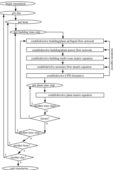
The whole system problem can now be stated as the co-ordinated solution of the domain equations under control action that links certain model parameters (e.g. room air temperature to the mass flow rate induced by a fan). Figure 4 summarises the ESP-r procedure, which is based on the itera-tive solution of nested domains. Given that the building time constants are generally greater than those related to the plant, the approach taken is to process the plant system at the same, or greater, frequency than the domains associated with the building. In this way, the plant equations may be solved for small time steps, to accurately repre-sent the effect of control action, while the more slowly evolving building may be solved less fre-quently. Where required, the processing frequen-cies may be matched and/or increased.

At each building-side time step, and for a given climate boundary condition, the air/liquid flow networks corresponding to the building and plant are established, control considerations imposed and the equations solved. Solution of these net-works give the air and working fluid flow rates throughout the building and within the plant sys-tem respectively.

The electrical power flow network representing building-side entities (e.g. lighting, small power,

photovoltaic facades etc) and plant components

(e.g. fans, pumps, CHP plant etc) is established, constrained by control action and the equations solved. The facility may be used to impose demand side actions on load consuming systems. (This network model and the preceding one for air/liquid flow may also be invoked at higher fre-quency from within the HVAC solution loop.)

The building-side, multi-zone matrix equation is then established using the latest estimates of the fluid/power flows and plant induced flux

per day

per hour

per building time-step

establish/solve building/plant air/liquid flow network

establish/solve building multi-zone matrix equation

per plant time-step

establish/solve plant matrix equation

iterate? begin simulation

another time-step?

another time-step?

another hour?

another day?

end simulation y

n

n

n

y

n

establish/solve CFD domain(s)

n y

establish/solve moisture flow matrix equation establish/solve building/plant power flow network

y

y

possible iterations

Figure 4: Iterative solution of nested domains.

injections/extractions. Equation solution is achieved as described previously to obtain the building’s temperatures and heat flows.

Using the newly computed intra-construction temperatures, the construction moisture flow matrix equation is established and solved. This gives the moisture distribution within the building fabric.

Using the building temperatures and air flow rates as boundary conditions, the CFD model is established and solved. This gives the intra-zone distribution of temperature, velocity, pressure and contaminants.

The building temperatures and air/liquid flow rates are then used, along with relevant control loops, to establish and solve the plant heat and mass flow matrix equations. Solution of these equations gives the plant temperatures and flow rates.

To orchestrate the process, domain-aware con-flation controllers are imposed on the different iterations. Consider, for example, the linking of the building thermal, network air flow and CFD models. This employs a controller that ensures that the CFD model is appropriately configured at each time-step (Beausoleil-Morrison 2001).

buoyant, fixed, fully turbulent or weakly turbu-lent). This information is then used to select appropriate surface boundary conditions, while the estimated eddy viscosity distribution is used to initialise thekandεfields. A second CFD sim-ulation is then initiated for the same time-step.

On the basis of the investigative simulation, the nature of the flow at each surface is evaluated

from the local Grashof (Gr) and Reynolds (Re)

Numbers, which indicate "how buoyant" and "how forced" is the flow respectively:

Gr/ Re2 << 1; forced convection effects over-whelm free convection

Gr/ Re2 >> 1; free convection effects dominate

Gr≈Re2; both forced and free convection

effects are significant

Where buoyancy forces are insignificant, the buoyancy term in the z-momentum equation is discarded to improve solution convergence.

Where free convection predominates, the

log-law wall functions are replaced by the Yuanet al

(1993) wall functions and constant boundary con-ditions imposed where the surface is vertical; oth-erwise a convection coefficient correlation is pre-scribed (this means that the thermal domain will influence the flow domain but not the reverse). Where convection is mixed, the log-law wall functions are replaced by a prescribed convection coefficient boundary condition.

Where forced convection predominates, the ratio of the eddy viscosity to the molecular vis-cosity (µt/µ), as determined from the

investiga-tive simulation, is examined to determine how tur-bulent the flow is locally:

µt/µ≤30:- the flow is weakly turbulent; the

log-law wall functions are replaced by a prescribed convection coefficient;

µt/µ> 30:- retain the log-law wall functions.

The iterative solution of the flow equations is re-initiated for the current time-step. For surfaces wherehc correlations are active, these are shared

with the building thermal model to impose the surface heat flux on the CFD solution. Where such correlations are not active, the CFD-derived convection coefficients are inserted into the build-ing thermal model’s surface energy balance.

Where an air flow network is active, the node representing the room is removed and new con-nection(s) added to effect a coupling with the appropriate domain cell(s) (Negra ˜o 1995, Clarke

et al 1995). A technique by Denev (1995) is

employed to ensure the accurate representation of both mass and momentum exchange in the situa-tion where CFD cells and network flow compo-nents are of dissimilar size.

Similar conflation mechanisms exist to enact informed ’hand-shaking’ between the other domain pairings.

FUTURE REQUIREMENTS

User interface aspects aside, the ESP-r approach to integrated building simulation is able to accom-modate many of the issues that underpin energy conscious building design. While the Open Source (www.opensource.org) nature of ESP-r should ensure that it continues to evolve in the light of new research findings, the real issue is whether the underlying approach is able to accommodate future user requirements. In some respects this is assured: a new method will only require the implementation of a new source term, the adjustment of existing equation coefficients or incorporating both together through a control function. Examples include the detailed mod-elling of ventilated facades, internal shading devices and time/location dependent heat injec-tions. In other cases an entirely new domain model may be required so that the issue becomes the ease with which the new model can be inte-grated.

This section identifies some upcoming mod-elling issues and considers how the ESP-r solu-tion approach may be evolved to accommodate them.

Domain solution developments Building thermal processes

The ESP-r model has proved to be resilient when applied to a range of problems over two decades. Recent work has focused on the implementation of phase change materials, while ongoing work is addressing the nuances of double skin facade modelling. In both cases no solver adaptations were required.

The system is also well adapted to the mod-elling of innovative components such as light sen-sitive shading devices and hybrid photovoltaics, requiring enhancements to the resolution of exist-ing models to allow, for example, slat angle adjustment in the former case and heat transfer surface geometry modelling in the latter.

Inter-zone air flow

At the present time ESP-r’s network air flow model is based on the steady-state line integration of the Navier-Stokes equation. When coupled with the building, oscillation problems may occur due to the numerical error. This issue can be resolved in two ways: by introducing a pressure capacity term into the mass balance equations; and by introducing transport delay terms to the network connections. Additionally, the modelling of contaminant concentration distribution can be carried out in parallel and/or coupled with the net-work air flow and building thermal models. Since it is a diffusive type system, with the convective terms predicted by the network air flow model, contaminant distribution may be evaluated as a scalar quantity and therefore the solution is straightforward.

The current theory may also be readily extended to handle higher level systems such as district heating, and problematic issues such as ’water hammer’ (via the introduction of a pres-sure capacity term).

Intra-zone air movement

Several developments may be readily applied to the CFD model: tunnel-type fans, as used in indoor car parks, can be modelled as free-stand-ing supply or extract points; while dampers and diffusers can be modelled by the imposition of a pressure boundary within a space. Such devices may be implemented through relatively simple coding modifications without the need to signifi-cantly modify the underlying solution procedure.

Other developments will require additional equations and so will impact upon the solution procedure. For example, the CFD technique is presently incapable of modelling small solid par-ticulates that have weight transport within the main air stream. Two particle dispersion/deposi-tion modelling methods are being considered for implementation: treating the particles as a contin-uum or particle tracing using Lagrange coordi-nate.

The modelling of fire/smoke requires that extra equations be added to handle combustion reac-tions and the transport of combustion products (e.g. via the implementation of mixture fraction or grey gas radiation transport models). Such adjust-ments can be readily implemented within the existing code since the governing equations are of diffusive type and so can be treated in the same way as the energy and species diffusion equa-tions. In conjunction with the network flow model, the transient distribution of fire and smoke may then be applied as a boundary condition for the prediction of the movement of occupants dur-ing a fire.

HVAC systems

The HVAC domain comprises models for each plant components, which may be based on the same or dissimilar theories. In this sense, the extensibility of the approach is unlimited: new modelling methods may be implemented as new products emerge.

The major issue confronting ESP-r is the gener-ation of the component models in the first place and the combination of the selected components to form a working HVAC system. To this end, two issues need to be addressed: the synthesis of com-ponent models from basic heat transfer/flow ele-ments and the automatic linking of the resulting models. The former issue is addressed by the

Primitive Part technique (Chow et al 1998)

whereby component models may be synthesised as and when required; while the latter issue might build upon previous research into object oriented HVAC (Tang 1996).

Further developments are also required in rela-tion to the connecrela-tion of HVAC and CFD domains, especially where the former impose complex flow patterns on the latter.

Domain interaction developments Occupancy interactions

It is well known that the effects of occupancy can vastly increase energy use. These effects arise from two avenues: behaviour (e.g. the occupants’ response to window opening) and attitude (e.g. the rejection of facilities on other than perfor-mance grounds). There is a need to explicitly model such behaviour and, in the context of ESP-r, two approaches are possible: ’typical’ interac-tions may be included within a controller that has authority to adapt the parameters of the affected domain models prior to solution; or, more realisti-cally, an occupancy response model may be intro-duced by which the response to stimulus is explic-itly represented. In both cases the aim is to address the distributed impacts of occupant actions (e.g. the impact on the network flow, CFD, thermal and lighting domains of window opening).

Micro-grids

that may be applied to switch certain loads within the context of renewable power trading. Such a facility will primarily interact with the building thermal, HVAC and electrical domains by acting to reschedule heating/cooling system set-point temperatures, and withholding/releasing power consuming appliances where acceptable.

Next generation

In the long term, additional solver developments may be implemented to bring about computa-tional efficiencies and thereby assist with the translation of simulation to the early design stage. For example:

1. additional, context-aware solution accelera-tors may be embedded within the solvers to con-trol their appropriate invocation;

2. parallelism may be introduced to allow the different domains to be established and solved in tandem to reduce simulation times; and

3. network computing might be exploited to allow different aspects of the same problem to be pursued at different locations as an aid to team working.

Such developments might well be built upon entirely new methods such as ’intelligent matrix patching’ whereby the coupling information between domain models are stored in a ’patch matrix’ allowing the numerical model of the cou-pling components to be activated only when the actual coupling takes place. Further, a greater level of coefficients management may be intro-duced to ensure that the matrix coefficients are only updated when required and otherwise never reprocessed. Such devices would lead to signifi-cant reductions in computing times.

CONCLUSIONS

This paper has summarised the distributed approach to domain solution as employed within the ESP-r system. Several possible technical developments were then outlined as required by new user demands that imply a need to extend and deepen the analysis scope.

ACKNOWLEDGEMENTS

The authors are indebted to the many individuals who have contributed to the ESP-r project since its inception in 1974.

REFERENCES

Beausoleil-Morrison I, 2000, The Adaptive Coupling of Heat and Air Flow Modelling within

Dynamic Whole-Building Simulation, PhD

The-sis, Glasgow: University of Strathclyde.

Chen Q and Xu W, 1998, A Zero-Equation

Turbulence Model for Indoor Airflow Simulation,

Energy and Buildings,28(2), pp137-44.

Chow T T, Clarke J A and Dunn A, 1998, The-oretical Basis of Primitive Part Modelling,

ASHRAE Trans.,104(2).

Clarke J A, 2001,Energy Simulation in

Build-ing Design (2nd Edn), London:

Butterworth-Heinneman.

Clarke J A, Dempster W M and Negra ˜o C,

1995, The Implementation of a Computational Fluid Dynamics Algorithm within the ESP-r

Sys-tem, Proc. Building Simulation ’95, Madison,

pp166-75.

Conte S D and de Boor C, 1972, Elementary

Numerical Analysis: an Algorithmic Approach,

New York: McGraw-Hill.

Denev J A, 1995, Boundary Conditions Related to Near-Inlet Regions and Furniture in Ventilated

Rooms, Proc. Application of Mathematics in

Engineering and Business243-8, Technical

Uni-versity of Sofia.

Kelly N J, 1998, Tow ard a Design Environment for Building-Integrated Energy Systems: The Integration of Electrical Power Flow Modelling

with Building Simulation,PhD Thesis, Glasgow:

University of Strathclyde.

Nakhi A E, 1995, Adaptive Construction Mod-elling Within Whole Building Dynamic

Simula-tion,PhD Thesis, Glasgow: University of

Strath-clyde.

Negra ˜o C O R, 1995, Conflation of Computa-tional Fluid Dynamics and Building Thermal

Simulation,PhD Thesis, Glasgow: University of

Strathclyde.

Patankar S V, 1980,Numerical Heat Transfer

and Fluid Flow, New York: Hemisphere.

Press W H, Flannery B P, Teukolsky S A and

Vettlering W T, 1986,Numerical Recipes: the Art

of Scientific Computing, Cambridge University

Press.

Tang D, 1996, Object Technology in Building

Environmental Modelling,Building and

Environ-ment,32(1), pp45-50.

Van Doormal J P and Raithby G D, 1984, Enhancements of the SIMPLE Method for

Pre-dicting Incompressible Fluid Flows, Numerical

Heat Transfer7, pp147-63.

Versteeg H K and Malalasekera W, 1995, An

introduction to Computational Fluid Dynamics:

The Finite Volume Method, England: Longman.

Walton G N, 1982, Airflow and Multiroom

Thermal Analysis,ASHRAE Trans.,88(2).

Yuan X, Moser A and Suter P, 1993, Wall Functions for Numerical Simulation of Turbulent

Natural Convection Along Vertical Plates, Int. J.