The environmental dimension of multifunctionality: economic analysis and implications for policy design

Full text

(1)Agrifood Research Repor ts 20. Agrifood Research Repor ts 20 Agrifood Research Reports 20. The Environmental Dimension of Multifunctionality: Economic Analysis and Implications for Policy Design Doctoral Dissertation Jussi Lankoski. Economics.

(2) Agrifood Research Reports 20 107 p., 5 appendices. The Environmental Dimension of Multifunctionality: Economic Analysis and Implications for Policy Design Doctoral Dissertation Jussi Lankoski. Academic Dissertation To be presented, with the permission of the Faculty of Agriculture and Forestry of the University of Helsinki, for public examination in Auditorium XII, Unioninkatu 34, Helsinki, on March 28th, 2003, at 12 o’clock.. MTT Agrifood Research Finland.

(3) Supervisor: Professor Markku Ollikainen, Department of Economics and Management, University of Helsinki, Finland Reviewers: Professor Richard N. Boisvert, Department of Applied Economics and Management, Cornell University, USA Professor Hervé Guyomard Agricultural Economics and Sociology Department, Institut National de la Recherce Agronomique (INRA), France Opponent: Professor Eirik Romstad Department of Economics and Social Sciences Agricultural University of Norway, Norway. ISBN 951-729-745-9 (Printed version) ISBN 951-729-928-1 (Electronic version) ISSN 1458-5073 (Printed version) ISSN 1458-5081 (Electronic version) www.mtt.fi/met/pdf/met20.pdf Copyright MTT Agrifood Research Finland Jussi Lankoski Publisher MTT Economic Research, Agrifood Research Finland, Luutnantintie 13, 00410 Helsinki, Finland www.mtt.fi/mttl Distribution and sale MTT Economic Research, Agrifood Research Finland, Luutnantintie 13, 00410 Helsinki, Finland Phone + 358 9 56 080, Fax + 358 9 563 1164 e-mail [email protected] Printed in 2003 Printing house Data Com Finland Oy Cover picture Copyright Yrjö Tuunanen/MTT. 1.

(4) The Environmental Dimension of Multifunctionality: Economic Analysis and Implications for Policy Design Jussi Lankoski MTT Economic Research, Agrifood Research Finland, Luutnantintie 13, FIN-00410 Helsinki, Finland, [email protected]. Abstract Multifunctional agriculture refers to the fact that agriculture produces jointly a number of commodity and non-commodity outputs, and some of these noncommodity outputs exhibit the characteristics of externalities and public goods. Thus, multifunctionality provides an integrated framework for the simultaneous consideration of multiple commodity and non-commodity outputs. Multifunctionality constitutes a complex problem from the perspective of policy design and implementation. Finding out the socially optimal bundle of multiple commodity and non-commodity outputs involves the identification of the important outputs as well as their relative significance, and policies conducive to multifunctional agriculture must simultaneously address several outputs, commodity and non-commodity ones. Moreover, the heterogeneous conditions under which agriculture operates create a spatial dimension in the supply of commodity and non-commodity outputs. That is, there are spatial differences in productivity and, hence, in the production costs of commodity and non-commodity outputs. Finally, there are trade-offs between the precision of the policy instruments and their information requirements and related administrative costs. The main objective of the present study was to contribute to the understanding of the implications of multifunctionality for effective agri-environmental policy design. The main research question addressed was the performance of various types of policy interventions in achieving the optimal bundle of multifunctional outputs under heterogeneous conditions. The scope of the present study was restricted to the environmental dimension of multifunctionality. Two commodity outputs and three environmental noncommodity outputs (nutrient runoffs, landscape diversity, and agrobiodiversity) were analysed, taking into account jointness and heterogeneity in their supply and the externality and public good aspects in their demand. In this study an analytical model was developed, and then empirical results were obtained by calibrating the model to Finnish data. First, the farmer's private optimum was compared to the social optimum where nutrient runoffs, landscape diversity, and agrobiodiversity were valued at their social marginal values. Next, solutions were developed for the first-best differentiated policy instruments and the second-best uniform and semi-uniform policy instruments. 3.

(5) Finally, farm income support measures and environmental cross-compliance schemes were analysed. The study brings out how the design of agri-environmental policies against the background of multifunctionality differs from the individual treatment of the various environmental effects of agriculture. Because of the joint production process, the levels of different multifunctional outputs are linked to each other. Hence, the regulation of one environmental effect necessarily influences the other environmental effects and agricultural production, as well as other dimensions of multifunctionality. These interactions need to be accounted for when designing policies inducive to multifunctionality. It was shown that the optimal policy with respect to multifunctional agriculture under heterogeneous land quality is to use the combination of a differentiated fertilizer tax and a differentiated buffer strip subsidy. The requirement for the use of differentiated instruments arises from the fact that the non-commodity outputs indirectly depend on the heterogeneous land quality through the size of the buffer strips and the amount of fertilizer used. Thus, the first-best solution requires that policy instruments vary over land quality and crop because non-commodity outputs do so. The social welfare difference between the first-best differentiated instruments and the second-best uniform instruments is FIM 64 (10.8 €) per hectare in the case of semi-uniform instruments (cropspecific but uniform with respect to land quality) and FIM 116 (19.5 €) per hectare in the case of fully uniform instruments. Regarding farm income support measures, the results show that pure acreage subsidy and pure producer price support perform poorly in promoting the environmental elements of multifunctional agriculture. However, the performance of these income support measures could be greatly improved by incorporating some environmental cross-compliance mechanisms into them. To sum up, the combination of differentiated policy instruments is needed to secure the production of the optimal bundle of multifunctional outputs under heterogeneous conditions. Index words: Agrobiodiversity, buffer strip, heterogeneity, landscape mosaic, land quality, nutrient runoffs. 4.

(6) Ympäristöllinen monivaikutteisuus: Taloudellinen analyysi ja merkitys politiikan suunnittelulle Jussi Lankoski MTT Taloustutkimus, Luutnantintie 13, 00410 Helsinki, [email protected]. Tiivistelmä Käsitteellä monivaikutteinen maatalous viitataan siihen, että maatalous ruoanja kuiduntuotannon lisäksi tuottaa muitakin yhteiskunnan hyvinvointiin vaikuttavia maaseutu- ja ympäristöhyödykkeitä. Tärkeimpiä monivaikutteisuuden ulottuvuuksia ovat ympäristön laatu, elintarvikkeiden huoltovarmuus ja maaseudun sosioekonominen elinvoimaisuus. Määritelmällisesti monivaikutteisuustuotosten tulisi syntyä yhteistuotosprosessissa varsinaisen tuotannon yhteydessä ja olla luonteeltaan selvästi ulkoisvaikutuksia ja julkishyödykkeitä. Monivaikutteisuus tarjoaa haastavan ongelman politiikan suunnitteluun ja toimeenpanoon. Etsittäessä optimaalista monivaikutteisuustuotosten kokonaisuutta on pystyttävä tarkastelemaan samanaikaisesti sekä varsinaista maataloustuotantoa että monivaikutteisuuden muita ulottuvuuksia. Tarkastelua vaikeuttavat vielä ulottuvuuksien riippuvuus toisistaan yhteistuotosprosessin kautta, maataloudelle tyypilliset heterogeeniset tuotanto-olosuhteet ja toimivien markkinoiden puuttuminen useilta monivaikutteisuustuotoksilta. Tämän tutkimuksen tavoitteena on lisätä tietoa monivaikutteisuuden merkityksestä maatalouspolitiikan ja maatalouden ympäristöpolitiikan suunnittelussa. Keskeisenä tutkimusongelmana on erilaisten politiikkatoimenpiteiden kyky saavuttaa yhteiskunnallisesti optimaalinen maatalouden monivaikutteisuus heterogeenisissä olosuhteissa. Tutkimus on rajattu monivaikutteisuuden ympäristölliseen ulottuvuuteen ja siinä analysoidaan kahden viljelykasvin ja kolmen ympäristöhyödykkeen yhteistuotosprosessia peltoekosysteemissä. Analysoitavat ympäristöhyödykkeet ovat agrobiodiversiteetti, maaseutumaiseman monimuotoisuus ja ravinnepäästöt. Tutkimuksessa on ensimmäisen kerran kehitetty sekä analyyttinen että empiirinen malli, joka tarjoaa integroidun viitekehyksen monivaikutteisuuden ulottuvuuksien tarkastelulle. Aluksi johdetaan edustavan viljelijän yksityinen optimi ja verrataan sitä yhteiskunnalliseen optimiin, jossa ympäristöhyödykkeitä arvostetaan niiden yhteiskunnallisten rajahaittojen ja rajahyötyjen mukaisesti. Seuraavaksi analysoidaan kolmentyyppisiä politiikkatoimenpiteitä: (i) firstbest eli lohko- ja kasvikohtaisesti erilaistetut lannoitevero ja suojakaistatuki, (ii) second-best eli osittain (vain kasvikohtaisesti) erilaistetut tai kokonaan erilaistamattomat politiikkatoimenpiteet ja (iii) käytännön politiikkatoimenpiteet eli perinteiset maatalouspolitiikan tulotukimudot kuten hintatuki ja hehtaarituki sekä tulotuet, joihin on liitetty ympäristökriteerejä tulotuen saannin. 5.

(7) ehdoiksi. Empiiriset tulokset saadaan kalibroimalla analyyttinen malli suomalaiseen havaintoaineistoon. Tutkimus tuo esiin sen, kuinka maatalouden ympäristöpolitiikan suunnittelu monivaikutteisuuden viitekehyksestä käsin poikkeaa maatalouden ympäristöasioiden yksittäisestä tarkastelusta. Yhteistuotosprosessin vuoksi eri monivaikutteisuustuotosten tuotannon taso on kytköksissä toisiinsa. Tämän seurauksena yhden ympäristöhyödyn tai -haitan sääntely aiheuttaa väistämättä muutoksia niin muissa ympäristöhyödykkeissä ja itse maataloustuotteiden tuotannossa kuin muissa monivaikutteisuuden ulottuvuuksissakin. Yhteiskunnallisesti optimaalisen monivaikutteisuuspolitiikan lähtökohdaksi tulevatkin räätälöidyt politiikkatoimenpideyhdistelmät, joissa toimenpiteiden taso asetetaan koordinoidusti. Tutkimuksen tuloksena on myös, että heterogeeniset olosuhteet vaativat heterogeenisen sääntelyn. Kun viljelysmaan laatu vaihtelee siten, että se vaikuttaa sekä viljelykasvien että ympäristöhyödykkeiden tuotantoon, yhteiskunnan näkökulmasta optimaalinen monivaikutteisuuspolitiikka on erilaistaa politiikkatoimenpiteiden taso heijastamaan näitä heterogeenisiä olosuhteita. Käytännössä tämä merkitsee lohko- ja kasvikohtaisesti erilaistettuja toimenpiteitä. Mikäli politiikkatoimenpiteet on erilaistettu vain osittain tai ei lainkaan, yhteiskunnallisesti optimaalista monivaikutteisuustuotosten määrää ei saavuteta. Tutkimuksen empiirisessä aineistossa tämä yhteiskunnan hyvinvointitappio epätarkempien ohjauskeinojen käyttämisestä oli 64 mk/ha (10,76 €/ha) kasvikohtaisesti erilaistetuilla toimenpiteillä ja 116 mk/ha (19,51€/ha) kokonaan erilaistamattomilla toimenpiteillä. Epätarkemmista toimenpiteistä koituva hyvinvointitappio on kuitenkin suhteutettava erilaistettujen politiikkatoimien vaatimiin suuriin hallinnointikustannuksiin. Lisäksi tutkimus osoittaa, että sekä puhdas hintatuki että hehtaarituki kuten CAP-kompensaatiotuki eivät edistä monivaikutteisuuden ympäristöllistä ulottuvuutta. Näiden toimenpiteiden kykyä ottaa monivaikutteisuus huomioon ja edistää sitä voidaan kuitenkin merkittävästi parantaa liittämällä niihin ympäristöehtoja. Asiasanat: Biologinen monimuotoisuus, heterogeenisyys, maaseutumaisema, ravinnepäästöt, suojakaista, viljelysmaan laatu. 6.

(8) Acknowledgements I am indebted to many persons and organisations that have supported my dissertation research and graduate studies. My sincere gratitude goes to my supervisor, Professor Markku Ollikainen. He provided excellent guidance and invaluable support throughout this research. I wish to thank the preliminary examiners of this dissertation, Professor Richard N. Boisvert and Professor Hervé Guyomard, for their insightful and constructive comments that improved the quality of the dissertation in several ways. Professor Eirik Romstad I thank for agreeing to become my public examiner. I am very grateful to Dr. Chiara Lombardini-Riipinen for her competent guidance and assistance in making empirical calculations in Mathematica. I also greatly benefited from discussions with Dr. Jyrki Aakkula, Professor Juha Helenius, Professor Anni Huhtala, Dr. Heikki Lehtonen, Professor Erik Lichtenberg and PhD Jukka Peltola. I wish to extend my thanks to all my colleagues both at the MTT Economic Research and at the Department of Economics and Management of the University of Helsinki for the practical and spiritual help that I received. Especially, I am thankful to Professor Jukka Kola and Professor Kyösti Pietola for their support throughout my research career. My thanks also go to Jaana Kola for her competent revision of the English of the dissertation manuscript, and to Jaana Ahlstedt for her efficient technical editing of the manuscript. I wish to express my gratitude for the financial support that I received for this research and my graduate studies from the Ministry of Agriculture and Forestry, Kyösti Haataja Foundation, August Johannes and Aino Tiura Foundation and Agronomiliitto. My parents Antti and Lea and my sisters Jaana and Kristiina have always supported me in many ways. For this I am very thankful. Finally, I thank my dear wife Leena for the multifunctional role that she played in this process, both in questions of substance and in those of encouragement and support. Helsinki, February 2003 Jussi Lankoski 7.

(9) Contents 1 Introduction ............................................................................................ 10 1.1 Background ..................................................................................... 10 1.2 Objectives and outline of the study ................................................. 12 1.3 Core concepts .................................................................................. 14 1.4 The context for multifunctionality in Finland ................................ 19 2 Environmental multifunctionality – Literature review .......................... 24 2.1 Special features in supply ............................................................... 25 2.1.1 Joint production ..................................................................... 25 2.1.2 Heterogeneity ......................................................................... 27 2.2 Special features in demand ............................................................. 29 2.2.1 Externalities and public goods ............................................... 29 2.2.2 Valuation ................................................................................ 32 2.3 Special features in policy design ..................................................... 35 2.3.1 Policy design for multifunctionality ...................................... 36 2.3.2 Policy design for selected non-commodity outputs............... 38 2.3.3 Policy design under heterogeneous conditions ...................... 41 2.3.4 Transaction costs ................................................................... 43 2.4 Conclusions ..................................................................................... 44 3 Socially optimal multifunctional agriculture ......................................... 45 3.1 Introduction ..................................................................................... 45 3.2 The model of crop production ......................................................... 46 3.2.1 Input use ................................................................................. 48 3.2.2 Land allocation ...................................................................... 51 3.3 Socially optimal provision of multifunctional outputs ................... 56 3.3.1 Agricultural diversity and runoff functions ........................... 56 3.3.2 Command optimum ............................................................... 58 8.

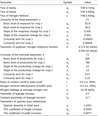
(10) 3.4 Numerical characterisation of multifunctional agriculture ............. 61 3.4.1 Parametric model ................................................................... 62 3.4.2 Numerical solutions ............................................................... 66 3.5 Conclusions ..................................................................................... 69 4 Policy design: Uniform and differentiated policy instruments .............. 71 4.1 Introduction ..................................................................................... 71 4.2 Optimal level of fertilizer tax and buffer strip subsidy ................... 72 4.2.1 Comparative statics of fertilizer tax and buffer strip subsidy ................................................................................... 72 4.2.2 Characteristics of the first-best policy instruments ............... 72 4.2.3 Optimal instruments and net support to agriculture .............. 74 4.3 Numerical solutions ........................................................................ 77 4.4 Conclusions ..................................................................................... 81 5 Income support measures and multifunctionality .................................. 82 5.1 Introduction ..................................................................................... 82 5.2 Private optimum in the presence of income support measures ....... 83 5.2.1 Input use ................................................................................. 83 5.2.2 Land allocation ...................................................................... 85 5.3 Numerical solutions ........................................................................ 87 5.4 Conclusions ..................................................................................... 93 6 Conclusions ............................................................................................ 94 6.1 Summary and main findings ........................................................... 94 6.2 Policy implications .......................................................................... 96 6.3 Limitations of the study and suggestions for further research ........ 97 References. ............................................................................................... 99. Appendices. 9.

(11) 1 Introduction 1.1 Background For some time it has been recognised that, besides the production of food and fibre, agriculture has other functions through which it contributes to social welfare. Jointly with the production of agricultural commodities, so-called noncommodity outputs arise. These include rural and environmental amenities, rural settlement and employment, and national food security. Sometimes also cultural and historic heritage values, food safety, and farm animal welfare are mentioned in this context. A new slogan, multifunctionality, has emerged in the international policy debate to capture these features of agricultural production. While the economic significance of agriculture has decreased for some time in a number of countries, income growth has resulted in a growing demand for many of the non-commodity outputs. Through domestic agricultural policies governments try to ensure that the provision of these outputs corresponds to that demanded by society. Thus, even though multifunctionality as a policy term is new, as an implicit concept in the context of domestic agricultural policy it is not entirely new since some countries have already taken into account selected non-commodity outputs of agriculture in their policy-making. Multifunctionality is important from the domestic policy perspective, but it is the implications of further liberalised agricultural trade on the multifunctional character of agriculture that have raised this issue to the forefront in the international debate. Some countries fear that further reductions in and constraints on domestic support would reduce the ability of governments to pursue their domestic non-commodity objectives, whereas other countries consider that multifunctionality is being used as a pretext for maintaining high levels of production-related support. Hence, the concept of multifunctionality and its use as a basis for concrete policy interventions has raised conflicting views among the WTO members. The most commonly cited elements of multifunctionality – environment, food security, and the viability of rural areas – were listed as legitimate non-trade concerns in the draft text on agriculture during the WTO Ministerial Meeting in Seattle in 1999. The non-trade concerns related to agriculture can be defined as domestic policy objectives that countries perceive to be threatened by the further liberalisation of agricultural trade (Burrell 2001). However, due to its controversial nature the term multifunctionality itself was not mentioned in the draft text of the WTO Ministerial Meeting, and thus it did not reach a formal status.. 10.

(12) It could be argued that the elements of multifunctionality are already covered through the agreed list of non-trade concerns and that the policy relevance of multifunctionality is in that sense vague. However, although multifunctionality and non-trade concerns overlap, there is a fundamental difference between these concepts that has important implications for policy design. Whereas multifunctionality provides an integrated framework for the simultaneous consideration of multiple commodity and non-commodity outputs, non-trade concerns are dealt with as separate issues. That is, each non-trade concern is separately linked to commodity production, but tradeoffs and complementarities between alternative non-commodity outputs are not explicitly recognised. Clearly, multifunctionality constitutes a complex problem from the perspective of policy design and implementation. Finding out the socially optimal bundle of multiple commodity and non-commodity outputs involves the identification of the important outputs as well as their relative significance, which in itself is a challenging task. Moreover, policies promoting multifunctional agriculture must address simultaneously several outputs, commodity and non-commodity, which have tradeoffs and complementarities in their supply. Even if some non-commodity outputs of agriculture have in cases been taken into account in national policy-making, they have been addressed indirectly through commodity-related interventions. Now they are to be addressed directly. All this is further complicated by the fact that the heterogeneous conditions under which agriculture operates bring into being a spatial dimension in both the supply of and demand for non-commodity outputs. There are spatial differences in productivity and, hence, in production costs of commodity and non-commodity outputs on the supply side, and spatial valuation differences on the demand side. Finally, there is the practical problem that the information requirements and related transaction costs for designing and implementing spatially differentiated interventions in order to maximise social welfare from optimal bundles of commodity and non-commodity outputs may be quite extensive, wherefore governments may be obligated to look for less effective solutions which are less information-intensive but which distort production decisions and thus trade. So far, the economic analysis of policy design for multifunctionality has mainly been conceptual. OECD (2001a) provides some preliminary policy guidance that is based on the working definition of multifunctionality and on the conceptual framework developed by the OECD. However, owing to the conceptual nature of the analysis, the guidance for policy design remains quite general; for example, whether policy intervention is warranted or not and what kind of policy interventions (coupled with or decoupled from commodity production) would most likely be efficient. Thus, it could be argued that due to the conceptual nature of the existing studies, the economic analysis of policy design for multifunctionality has not yet been rigorously conducted. A major. 11.

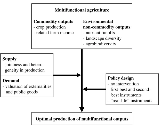
(13) problem in the previous literature is that the commodity and non-commodity outputs have not been rooted in an integrated analytical and empirical framework in which the multiple commodity and non-commodity outputs are considered accurately and simultaneously.. 1.2 Objectives and outline of the study The objective of this study is to contribute to the understanding of the implications of multifunctionality for effective agri-environmental policy design. The main research question addressed is how various types of policy interventions perform in achieving the optimal bundle of multifunctional outputs under heterogeneous conditions. The rigorous treatment of jointness between commodity and non-commodity outputs and the related implications for policy design under heterogeneous conditions requires that input use and land use are endogenous in the analysis so that farmers’ responses to policy interventions in both intensive and extensive margins can be determined. Lichtenberg (1989, 2000) provides an excellent core for examining farmers’ input use and land allocation choices under heterogeneous conditions (heterogeneous land quality). However, his model does not have a spatial structure, which plays an important role in the analysis of such non-commodity outputs as landscape diversity and agrobiodiversity. The present study covers all three aspects: endogenous input use and land allocation, heterogeneity, and spatiality. Figure 1 illustrates the contents of the study. The study focuses on two commodity outputs and three environmental non-commodity outputs of multifunctional agriculture. These are considered simultaneously, taking into account the special features of jointness and heterogeneity in the production, and externality and public good aspects in demand. In order to achieve the optimal production of these multifunctional outputs, various policy solutions are examined. The starting point for the analysis is the conceptual framework on multifunctionality developed by the OECD (2001a). However, the present study attempts to move from concepts to a formal analysis and from there further to empirical applications. This is done by developing an integrated analytical and empirical framework that provides a sound basis for policy design and evaluation. Of the non-commodity outputs of multifunctional agriculture, the scope of the present study is restricted to the environmental dimension of multifunctionality. There are several reasons for this. First, the environmental dimension is the. 12.

(14) Multifunctional agriculture Commodity outputs - crop production - related farm income. Environmental non-commodity outputs - nutrient runoffs - landscape diversity - agrobiodiversity. Supply - jointness and heterogeneity in production Policy design - no intervention - first-best and secondbest instruments - “real-life” instruments. Demand - valuation of externalities and public goods. Optimal production of multifunctional outputs. Figure 1. Components of the study.. least controversial one in the international debate. Second, the joint production process is apparent in this dimension. Third, the environmental non-commodity outputs clearly possess the characteristics of externalities or public goods, some of them being in fact pure public goods. The analytical sections of the present study are generally applicable, but the empirical parameters of the parametric model apply to Finland only. The study is structured as follows. Chapter 1 of the study (introduction) continues with a short presentation of the key concepts used in the study. It also describes the context for multifunctional agriculture in Finland. Chapter 2 (literature review) discusses the supply, demand and policy aspects that are specific to multifunctional agriculture. Chapters 3, 4, and 5 constitute the core of the study. They examine the optimal provision of multifunctional outputs without government intervention (Chapter 3), the use of differentiated (first-best) and uniform (second-best) policy instruments for promoting multifunctional agriculture (Chapter 4), as well as some “real-life” policy instruments (Chapter 5). All these are investigated both analytically and by means of an empirical application with Finnish data. Chapter 6 concludes the study and discusses its main findings, policy implications, and limitations.. 13.

(15) 1.3 Core concepts The core concepts and terms used in the present study are defined in this section. The aim is to provide a quick overview rather than a comprehensive discussion, since some of the concepts presented here will be further elaborated and discussed in the literature review in Chapter 2. In the present study the terms multifunctionality, multifunctional agriculture and the multifunctional character of agriculture are used interchangeably. As there is no universally accepted definition for the concept of multifunctionality, a “working definition” provided by the OECD (2001a) is adopted. According to this definition, the fundamentals of multifunctionality are: (i) the existence of multiple commodity and non-commodity outputs that are jointly produced (ii) the fact that some of the non-commodity outputs exhibit the characteristics of externalities or public goods Hence, multifunctional agriculture may be defined as an economic activity which, besides its primary function of producing agricultural commodities, affects social welfare by producing multiple positive or negative non-commodity outputs jointly with the commodity production. Thus, in economic terms, multifunctional agriculture produces jointly private goods, public goods, and positive or negative externalities. It is worth noting that agriculture is by no means the only economic activity with multifunctional characteristics. For example, forestry provides several non-commodity outputs jointly with timber production. However, in the present study the term multifunctionality refers only to the joint production of noncommodity outputs with agricultural commodities. The significance of forestry to Finnish farms and the significance of farmers as forest owners in Finland nevertheless attach an interesting feature to the multifunctional character of Finnish agriculture. Finnish farmers provide non-commodity outputs such as landscape diversity, biodiversity, and viability of rural areas both through multifunctional agriculture and multiple-use forestry. Farmers’ management decisions with respect to agricultural land and production practices, but equally those with respect to forested land and timber harvesting, play a crucial role in the supply of several non-commodity outputs in rural areas. Consequently, the distinction between the non-agricultural provision of non-commodity outputs and that of their agricultural provision is somewhat vague because the same management unit shapes the provision of non-commodity outputs from both agriculture and forestry.. 14.

(16) Commodity outputs refer to agricultural commodities that are private goods. These include crops, farm animal products, fibres, energy plants, and so on. Non-commodity outputs, in turn, refer to non-market goods that arise as a side effect of the commodity production, such as landscape and environmental amenities. Joint production or jointness refers to a situation where two or more outputs are produced interdependently so that a change in the supply of one output affects the levels of the other outputs. According to the OECD (2001a), three frequently distinguished causes for jointness are (i) technical and biological interdependencies in the production process (ii) non-allocable inputs (iii) allocable inputs that are fixed at the firm level One example of a technical interdependence between commodity and non-commodity outputs is fertilizer use, which results in both increased yields and increased nutrient runoffs. The joint production of milk and manure, in turn, provides an example of a non-allocable input (cow). An example of jointness due to allocable inputs that are fixed at the firm level in the short run is the allocation of agricultural land between commodity production and wildlife habitat, such as conservation headlands. According to Baumol and Oates (1988: 17-18), there are two conditions for an externality. First, “an externality is present whenever some individual’s utility or production relationships include real variables, whose values are chosen by others without particular attention to the effects on this individual’s welfare”. Second, “the decision maker whose activity affects others’ utility levels or enters their production function, does not receive (pay) in compensation for this activity an amount equal in value to the resulting benefits (or costs) to others”. Thus, in brief, an externality can be defined as an uncompensated effect on a utility function or production set. The eutrophication of surface waters due to nutrient runoffs is an example of a negative externality produced by agriculture. A pure public good possesses the following characteristics: it is non-rival in consumption and yields benefits that are non-excludable (Callan and Thomas 1996). Non-rivalry means that one agent’s consumption of the good does not preclude that of the others. In other words, there is a zero marginal cost for an additional consumer of the good (Stiglitz 1988). Non-excludability means that it is impossible or prohibitively costly to exclude agents from consuming the good. Thus, because of non-rivalry it is not desirable and because of non-excludability it is not feasible to ration the use of the public good (Stiglitz 1988). 15.

(17) The non-use values of landscape and agrobiodiversity can be regarded as examples of pure public goods. The environmental dimension of multifunctionality or environmental multifunctionality refers to the joint production of commodities with environmental non-commodity outputs. The latter include positive non-commodity outputs, such as landscape diversity and agrobiodiversity, but also negative ones, such as impairment of the groundwater and surface water quality due to nutrient and pesticide leaching and runoffs, as well as loss of wildlife due to the use of chemicals and fragmentation and loss of habitats. The environmental non-commodity outputs, however, may also have indirect effects on the other dimensions of multifunctionality. For example, the attractiveness of rural areas for both the rural and urban population is affected by environmental quality and by landscape amenities (OECD 2001a). Through the natural resource base and the productive capacity of agriculture, environmental outputs, such as erosion and agrobiodiversity, may also affect food security as long as domestic production is regarded as an important part of this. According to the Convention on Biological Diversity (UNEP 1992), biological diversity or biodiversity is the variability among all living organisms from all sources, including terrestrial, marine and other aquatic ecosystems, and the ecological complexes of which they are a part. Agrobiodiversity is that part of biodiversity which relates to agriculture and agro-ecosystems. Like biodiversity, this can also be described at three fundamental levels: the diversity of ecosystems, species, and genes. Qualset et al. (1995) define agrobiodiversity to include all crops and livestock and their wild relatives, as well as all the interacting species of pollinators, symbionts, parasites, predators, and competitors. Beyond its role in the production of food and fibre, agrobiodiversity has multiple functions in agro-ecosystems. These include the recycling of nutrients, the regulation of hydrological processes, the control of microclimate, the regulation of undesirable organisms, and the detoxification of noxious chemicals (Altieri and Nicholls 1999). Swift and Anderson (1994) divide the biotic components of agro-ecosystems into three types: productive biota such as crops and livestock, resource biota that increase the productivity of the agro-ecosystem, such as pollinators and soil biota, and, finally, destructive biota such as weeds, pests, and pathogens. Gliessman (2000) defines an ecosystem to be a functional system of complementary relations between living organisms and their environment, delimited by arbitrarily chosen boundaries, which in space and time appear to maintain a steady, yet dynamic equilibrium. Whereas the structure of an ecosystem refers to its parts and their relationships, its function refers to the dynamic processes occurring within the ecosystem. An agroecosystem can be defined as a site of agricultural production that is understood as an ecosystem, for example, a group 16.

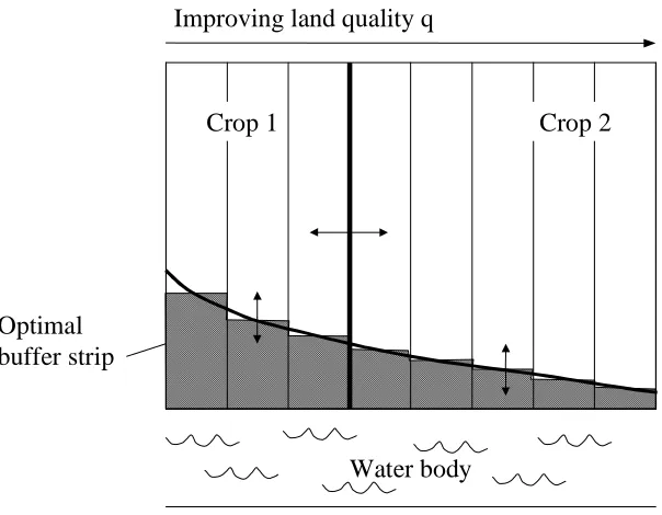
(18) of farms in the context of a watershed, an individual farm, or a farm field (Gliessman 2000). A fundamental feature of agroecosystems, compared to natural ecosystems, is the human intervention that usually aims to reduce species diversity in order to obtain the largest possible yield of the cultivated crops (Swift and Anderson 1994). Swift and Anderson (1994) subdivide a field ecosystem into the following components: (i) the plant subsystem, including the cultivated crop, weeds, and legumes and their obligatory pathogens and symbionts, (ii) the herbivore subsystem, including farm animals, predators, parasites, and parasitoids, and (iii) the soil or decomposer subsystem, including soil organic matter, soil micro-organisms such as bacteria, fungi, and algae, and micro-, meso-, macro- and megafauna (earthworms). The functions of a field ecosystem refer to processes such as the flow of energy and the cycling of nutrients (biogeochemical cycles), such as carbon and nitrogen (Swift and Anderson 1994). According to the OECD (2001b), agricultural landscapes are the visible outcomes that result from the interaction between commodity production, natural resources, and the environment. They include amenity, heritage, cultural, aesthetic, and other societal values. Three essentials of agricultural landscapes are their (i) structure or appearance, for instance, flora, fauna, habitats, ecosystems, crops, hedges, and farm buildings, (ii) cultural, environmental, and economic functions, and (iii) value, that is, society’s valuation of landscape. The structure of the spatial mosaic of a landscape and its effects on ecological systems, patterns, and processes is the focus of landscape ecology (Wiens 1995). The landscape mosaic can be described with the help of three types of spatial elements: patches, corridors, and background matrices (Forman 1995). In general terms, the spatial structure of the landscape is associated with the composition (number and occurrence) and configuration (distribution and spatial character) of different landscape elements (Eiden et al. 2001). Buffer strips and field boundaries are semi-natural habitats adjacent to the crop. In agricultural landscapes they constitute linear elements which form a network of corridors through which organisms can move between larger habitat patches. A field boundary can be defined as a strip of semi-natural vegetation bordering an arable field. Field boundaries are important as they comprise the largest area of semi-natural vegetation in modern arable landscapes and provide food, shelter, nesting, and overwintering sites for most of farmland wildlife (Kleijn 1997). A buffer strip is a managed, uncultivated area that is covered by perennial vegetation and located between the arable land and a water body. Buffer strips serve both ecological and environmental purposes as they promote agrobiodiversity and protect surface waters from nutrient and pesticide runoffs. Important factors affecting the botanical diversity of field boundaries 17.

(19) and buffer strips include the nutrient and herbicide load from the adjacent cropland, disturbance by farming operations, mowing and removing of the cuttings, and the width of the boundary or the buffer strip. Low disturbance levels, low agro-chemical load, removing of the cuttings, and sufficient width maximise botanical diversity (see e.g. Kleijn 1997, Kleijn and Snoeijing 1997, Ma et al. 2002, Schippers and Joenje 2002). According to Gilliam et al. (1997), buffer strips are very effective in the removal of sediment-associated nitrogen from surface runoff and nitrate from subsurface flows, and removals of 50–90% have been common. However, the effectiveness of buffer strips in removing nutrients from surface water and groundwater depends highly on hydrology. For example, surface flows should occur as a sheet flow rather than as focused flows, and groundwater should move at a slow speed through the buffer in order for nitrates to be effectively removed (Correll 1997). According to Hill (1996), vegetation uptake and microbial denitrification are the two major mechanisms in buffer strips for removing nitrates from subsurface water, but the relative importance of these two processes is uncertain. Moreover, as pointed out by Gilliam et al. (1997), the increased denitrification in buffer strip areas may trade water pollution for atmospheric pollution due to the increased generation of N2O. It is also important to note that buffer strips only reduce the surface runoff of nutrients but not runoff through drainage pipes. In Finnish experiments, 50–75% of the total nitrogen loss from cultivated fields occurred through drainage pipes (see e.g. Turtola and Jaakkola 1987, Turtola and Puustinen 1998). Nutrients, chiefly nitrogen, phosphorus, and potassium, are important inputs in agricultural production systems. Of the three main nutrients, nitrogen and phosphorus may cause water quality problems in surface water and groundwater. Runoff refers to nutrient transportation over the soil surface by rainwater and melting snow, whereas leaching refers to the transportation of nutrients through the soil by percolating rain and melting snow (Ribaudo et al. 1999). Nitrogen, in the form of nitrate, is easily soluble and very mobile in the environment, but phosphorus is relatively immobile and may build up in the soil over time. Nitrogen is transported from fields to water bodies through both surface runoff and leaching, or through drainage. Phosphorus is transported from fields to water bodies in particulate form and in dissolved form through surface runoff (Hanley 1990, NRC 1993, Ribaudo et al. 1999). Point source pollution refers to discharges at a specific location through a pipe, out-fall, or ditch. Nonpoint source pollution (NPSP), or dispersed or diffused pollution refers to pollution that affects waters in a more diffuse way and is difficult to trace back to a precise source. Nutrient runoff from agriculture is typical nonpoint source pollution, since the runoff does not emanate from a single point except in the case of drainage but leaves the field in so many places that an accurate monitoring of each source would be prohibitively expensive (Ribaudo et al. 1999). 18.

(20) 1.4 The context for multifunctionality in Finland When discussing a topic such as multifunctionality which is composed of several elements, it is important to keep in mind the topic in its entirety to maintain an appropriate perspective on individual issues. Therefore, this section outlines some major socio-economic and environmental features of multifunctional agriculture in Finland1. The aim of the section is to provide some background on the substance for the analysis and to illustrate the relevance of the selected commodity and non-commodity outputs in a wider context. Thus, this description draws from the specific case of Finland to provide a context for the empirical applications in Chapters 3, 4, and 5. The data concern mainly the year 1999, as do the empirical data in Chapters 3, 4, and 5. Finland is one of the world’s northernmost agricultural countries. Agricultural land covers only 8% of the surface area of Finland, but Finland is the EU Member State with the largest percentage (98.5%) of rural areas. Depending on the definition of countryside, between 1.2 and 1.6 million Finns, or 23 to 32% of the population, live in rural areas. (MAF 2001a). Finnish agriculture is mainly based on relatively small, privately owned family farms. A notable feature of Finnish farms is that 95% of all active farms own forests; in fact, 34% of Finnish forests are owned by farmers. (MAF 2001a). In 1999 the share of agriculture in GDP was 1.2%, but the importance of the total food chain in the national economy is much higher. The share of agricultural support in the gross return on agriculture was about 40% in 1999. The EU contributed a little over a third of this, while the rest was covered by national financing. In 1999 the share of agriculture in the employed labour force was about 5%. (MTTL 2000). The significance of agriculture in the Finnish economy has been decreasing and production growth has been much slower than in the other sectors of the economy (MTTL 2000). The number of people living in rural areas and gaining their livelihood from agriculture has been shrinking fast (MAF 2001a). The number of active farms has fallen from 129,000 in 1990 to 82,000 in 1999. At the same time, the average farm size has been on the increase. During the EU membership, that is, since 1995, the production structure has changed rapidly as the share of animal husbandry farms has fallen, while the share of crop farms has increased. In 1999, 43% of active farms cultivated arable crops; barley accounted for about 30% and wheat about 5% of the total cultivated area. (MTTL 2000). 1. For the assessment of the social costs and benefits of multifunctional agriculture in Finland see Yrjölä and Kola (2001).. 19.

(21) All in all, agriculture remains the most important economic activity in rural areas, even though both the number of farms and the number of people they employ are declining (MAF 2001a). However, the contribution of agriculture to regional economies and employment varies between regions. In 1999 the share of agriculture in GDP and employment was the highest in South Ostrobothnia (7–8% in GDP and 12% in employment) and the lowest in Uusimaa (0.2% in GDP and 0.8% in employment). (MTTL 2001). Nutrient runoffs and the resulting eutrophication of surface waters can be regarded as a major negative externality of Finnish agriculture. Agriculture is the main source of both nitrogen (43%) and phosphorus (62%) runoffs into surface waters (Valpasvuo-Jaatinen et al. 1997). Hence, one of the major objectives of Finland in the application of the European Union’s agri-environmental regulation EEC 2078/92 has been the reduction of nutrient runoffs. The longterm effects of the agri-environmental programme for 1995–99 (The General Agricultural Environment Protection Scheme) have been expected to amount to a 20% to 40% reduction of both nitrogen and phosphorus runoffs. In addition to this agri-environmental programme, the Finnish Government has issued a Resolution on water protection targets to 2005. The main goals of the Resolution are the reduction and prevention of eutrophication. Nutrient runoffs from agriculture should be reduced by 50% (nitrogen from 30,000 to 15,000 tons per year and phosphorus from 3,000 to 1,500 tons per year) from 1993 levels by the year 2005. Moreover, in the new agri-environmental programme for 2000– 2006 improvement in the quality of surface water through reductions in nutrient runoffs is still considered one of the most important policy objectives. Although soil erosion is not a significant problem, the mechanisation of agriculture and the use of heavy field machinery on wet soils has resulted in soil compaction and related soil erosion in some areas of Finland, which has increased phosphorus and sediment runoffs into surface waters. Due to the climatic conditions, that is, the hostility of the cold climate to many pests, pesticide use per hectare is very low in Finland. Pesticide runoffs in Finland have been estimated to vary between 0.1% to 1% of total use, depending on the pesticide used and on weather conditions (Laitinen et al. 1996). Pesticide contents in water bodies occasionally exceed the limits set for drinking water. Pesticide residues in foodstuffs have not been a problem in Finland, since the amount of residues has consistently been lower than the limits set for residues (Miettinen et al. 1997). Between 1990 and 1999, greenhouse gas emissions from agriculture decreased from 10.2 to 7.6 million tons in carbon dioxide equivalent. In 1999 agriculture accounted for 10% of total emissions in Finland. The share of agriculture has been estimated to be 2% of carbon dioxide, 40% of methane, and 50% of ni-. 20.

(22) trous oxide emissions (MAF 2001b). Of ammonia emissions in Finland agriculture accounts for 90%, wherefore reducing the amount of ammonia released from manure storing and spreading has been one of the goals of the agri-environmental programme (Grönroos et al. 1998). Over the past 50 years agricultural landscapes in Finland have become increasingly homogeneous due to the structural change and the mechanisation, rationalisation, and intensification of production. Rationalisation through subsurface drainage and the removal of small-scale elements (trees, ponds, hedges) and forest islands has resulted in more geometric field parcels with inevitably less value for landscape diversity and agrobiodiversity. The decline in the number of linear landscape elements (ditch banks and arable field borders adjacent to non-arable land) is largely explained by the replacement of open field ditches by subsurface drainage. At the national level, subsurface drainage has replaced, on the average, 500 m/ha of open ditches (Ruuska and Helenius 1996). The maintenance of diverse agricultural landscapes is of particular concern in Finland, since only 8% of the land area is used for agriculture. Although forestry also provides several non-commodity outputs in rural areas, not all of them are substitutes for those of agriculture. This is especially the case with respect to biodiversity and landscape diversity. Most of the threatened species in Finland live either in forest habitats or in agricultural habitats, and neither of them are substitutes for each other. Also in terms of landscape diversity, forestry may be a poor substitute for the landscape provision of agriculture. For example, the results of a survey by Hietala-Koivu et al. (1999) show that afforestation (refers to the establishment of forest cover to land that was not previously forested, e.g. agricultural land) and land abandonment are considered the most important factors that decrease the scenic value of landscapes. This is confirmed by the study of Tahvanainen et al. (1996), who conducted an interview survey on the effect of gradual afforestation on the scenic beauty of 32 different rural landscapes in Finland. The scenic beauty was considered to decrease along with the increasing intensity of afforestation. However, moderate afforestation could have a positive effect on scenic beauty. The more attractive the original landscape was the greater the negative effect of afforestation was found to be. Traditional biotopes, such as dry meadows and pastures, have the greatest number of species diversity in Finnish landscapes. The botanical diversity of these habitats has benefited from grazing and mowing (Pitkänen and Tiainen 2001). Specialisation in crop farming and the associated decrease in animal husbandry and grazing animals has resulted in such a dramatic decline in the total area of meadows and pastures that less than 20,000 hectares of valuable agricultural heritage environments remain (Heritage Landscapes Working Group 2000). According to Pykälä and Alanen (1996), species living in heritage land-. 21.

(23) scapes constitute 75% of all threatened species in agricultural landscapes. Because of the decline in the area of traditional biotopes, the importance of field boundaries and buffer strips for overall agrobiodiversity has increased. According to Rassi et al. (1991), one out of 4 bird, 21 insect and 14 vascular species that are endangered have suffered from the indirect effects of herbicides, the disappearance of boundary habitats, and autumn ploughing. Although the species diversity of agricultural environments has been on the decrease, there have also been some changes in agricultural practices that promote agrobiodiversity. Most of these positive changes have been introduced by the Finnish agri-environmental programme, like buffer strips, the management of field boundaries, limits on fertilizer use, as well as requirements relating to pesticide use and plant cover during winter. In addition to these so-called basic measures of the agri-environmental programme, there are special contracts relating to traditional biotopes, the promotion of biodiversity, and the management of landscapes. Figure 2 summarises some key data on the environmental and socio-economic significance of Finnish agriculture.. Share of Finnish agriculture in... GDP. 1,2. employment. 5 8. land use forest ownership. 34. nitrogen runoffs. 43. phosphorus runoffs. 62. greenhouse gases. 10 90. ammonia emissions 16,7. threat to species 0. 20. 40. 60. 80. 100. Percentage Figure 2. Selected indicators for the significance of Finnish agriculture in 1999 (MTTL 2000, MAF 2001a, Valpasvuo-Jaatinen et al. 1997, Grönroos et al. 1998, and Rassi et al. 1991).. 22.

(24) To conclude, the economic significance of agriculture is small from the national perspective, although its local socio-economic role in rural areas is crucial. At the same time, the environmental significance of agriculture is great in many respects. Moreover, since Finnish farmers are also an important group of forest owners in Finland, they have a twin role as custodians of multifunctional agriculture and multiple-use forestry. Therefore, the agricultural and silvicultural decisions and production practices of Finnish farmers are important in shaping the occurrence of several externalities and the provision of many public goods in Finland.. 23.

(25) 2 Environmental multifunctionality – Literature review This chapter reviews the literature relating to the environmental dimension of multifunctionality. It comprises three main sections: special features in the supply of, demand for, and policy design for environmental multifunctionality. This structure arises from the conceptual framework provided by the OECD (2001a), which this study makes use of. In this framework, a series of questions related to jointness on the supply side, public good characteristics on the demand side, and the possibility of the non-governmental provision of the noncommodity outputs are posed in order to arrive at appropriate policy guidance for multifunctionality. As noted by the OECD (2001a), the particularities in the supply and demand of multifunctional outputs are crucial for any discussion on policy implications. On the one hand, if there were no jointness in the production of multifunctional outputs, the non-commodity outputs could be supplied independently of the commodity production. On the other hand, if there were functioning markets for the non-commodity outputs, supply and demand would meet through those markets. In both cases, environmental multifunctionality becomes a non-issue from the policy perspective2. The literature review is geared to serve the analysis presented in Chapters 3 to 5. As such, it focuses on aspects that are specific to the environmental dimension of multifunctional agriculture. The examples presented are also selected so as to relate to the non-commodity outputs analysed in Chapters 3 to 5, that is, nutrient runoffs, landscape diversity, and agrobiodiversity. It should be noted that as an explicit topic of investigation, policy design for multifunctionality has been the subject of very little formal economic analysis. Notable contributions include Peterson et al. (1999), Romstad et al. (2000), Boisvert (2001), Guyomard and Levert (2001), OECD (2001a), and Vatn (2002). There are, nevertheless, a number of studies that shed light on the various individual aspects of multifunctionality. For example, there is a growing economic literature on the policy design for controlling nutrient runoffs.. 2. Naturally, public policy may be needed also in the case of non-joint non-commodity outputs. However, in this case there may be no policy link between promoting the non-commodity outputs and international trade flows (OECD 2001a).. 24.

(26) 2.1 Special features in supply As noted in Chapter 1, the existence of multiple commodity and non-commodity outputs that are jointly produced is a fundamental feature of multifunctionality (OECD 2001a). Joint production or jointness is a key feature in the supply side of multifunctionality and it implies that there are interdependencies in production so that a change in the supply of one output affects the levels of the other outputs. Hence, the supply of commodity and non-commodity outputs needs to be analysed within the joint production framework. It is noteworthy that joint production is adopted as the starting point in almost all economic analysis which explicitly examines multifunctionality, perhaps owing to the framework and working definition provided by the OECD (2001a). Another important feature on the supply side of environmental multifunctionality has to do with spatial differences in supply. That is, the quantity, quality, and composition of multifunctional outputs differ between and within countries due to heterogeneous conditions. These heterogeneous conditions which affect the nature of jointness and the optimal bundle of commodity and non-commodity outputs are termed “site productivity” by the OECD (2001a).. 2.1.1 Joint production According to Shumway et al. (1984), even though technical interdependence is generally regarded as the primary cause of jointness, also allocable fixed (or quasi-fixed) inputs, such as land, may cause jointness. In fact, Shumway et al. argue that jointness caused by allocable inputs is especially typical for agriculture as many farms produce more than one output, the amount of land devoted to each crop can easily be distinguished, and the amount of land is usually fixed in the short run (Shumway et al. 1984). Following Lau (1972), Shumway et al. (1984) make a distinction between jointness and nonjointness as follows. For technology to be nonjoint in inputs requires that the profit function is additively separable in output prices: m. π = ∑ pi G i (r / pi ) , where Gi is the individual profit function for the i:th outi =1. put, pi is the i:th product price, and r is the vector of input prices. Now the distinction between jointness and nonjointness is given by the supply response of the ith output to the price of the jth output, that is, for nonjointness ∂y i∗ / ∂p j = 0 and for jointness ∂y i∗ / ∂p j ≠ 0 where (i ≠ j ) . Thus, for instance,. there is jointness (nonjointness) in the production of barley and wheat if the supply of barley responds (does not respond) to the price of wheat.. 25.

(27) Lynne (1988), in his comment to Shumway et al. (1984), proposes a distinction between “jointness in technology” and “jointness in supply” so that jointness in technology refers to technical interdependence and jointness in supply to behavioural interdependence. According to Lynne (1988), jointness, as traditionally represented, occurs only with non-allocable inputs and is synonymous with technical interdependence. However, fixed but allocable inputs may cause behavioural jointness in supply even if outputs are technically independent (nonjoint). In their reply to Lynne (1988), Shumway et al. (1988) refer to Lynne’s argument that production functions underlying joint production do not contain allocable inputs. They provide an example of the allocation of inputs for two crops where pesticide, which is a fully allocable input, applied to one crop in one field affects the yield of the other crop in an adjoining field. Thus, Shumway et al. argue that the production functions of these crops are not technically independent. In the subsequent contributions to the role of fixed but allocable inputs as a cause of joint production, Moschini (1989) and Leathers (1991) clarify the discussion through the notion of normal inputs and the cost function approach, respectively. Beattie and Taylor (1985) define the technical interdependence of two outputs as follows. Technical interdependence between two outputs produced from one allocable input can be viewed as the change of the marginal productivity of an input in the production of one output when the level of the other output changes. Thus, according to Beattie and Taylor (1985), if the multioutput production function is given by x = g ( y1 , y 2 ) , y1 and y2 are technically complementary if. ∂ 2 x / ∂y1∂y 2 ≡ g 12 < 0 , technically competing if ∂ 2 x / ∂y1 ∂y 2 ≡ g 12 > 0 , and technically independent if ∂ 2 x / ∂y1∂y 2 ≡ g12 = 0 . That is, technical interdependence is present if one output is increased and that results in the change of the inverse marginal productivity of the input use for another output (Beattie and Taylor 1985). Beattie and Taylor (1985) further define the economic interdependence of two outputs as follows. Two outputs are economically interdependent if a change in the price of one output affects the supply of the other output. In other words, two outputs yi and yj are economically competing if ∂y i∗ / ∂p j < 0 , economically complementary if ∂y i∗ / ∂p j > 0 , and economically independent if. ∂y i∗ / ∂p j = 0 for i, j =1,2 and (i ≠ j ). According to Boisvert (2001), the three commonly distinguished causes for joint production (technical interdependencies in the production process, non-allocable inputs, and allocable inputs that are fixed in the short run at the firm level) are also representative for jointness between most commodity and non-com26.

(28) modity outputs. However, these three sources of output interdependence may arise in various combinations and proportions, and it is unlikely for jointness to occur in fixed proportions (Boisvert 2001). Fertilizer or pesticide use that results in the joint production of commodities and nutrient or pesticide runoffs is one example of a technical interdependence between commodity and non-commodity outputs. Technical interdependencies are the source of many negative environmental externalities of commodity production, such as the nutrient and pesticide runoffs mentioned above, leaching, soil erosion, and greenhouse gas emissions. However, changes in farming technologies and practices may modify the composition of the commodity and non-commodity output bundle. (OECD 2001a). The joint production of meat and landscape by grazing cattle provides an example of a non-allocable input. In this case, multiple outputs arise from the same input, but they are rarely produced in fixed proportions, and so using different production methods may change the proportions (OECD 2001a). Land allocation between commodity production and abatement activities such as buffer zones represents an example of jointness which is due to allocable inputs that are fixed at the firm level in the short run. Boisvert 2001 provides an example where agricultural land is simultaneously an allocable and nonallocable input: it is allocable between two commodities but non-allocable between these commodities and landscape amenities. By taxing or subsidising the farmer, Boisvert demonstrates the economic significance of joint production of commodity and non-commodity outputs, regardless of the cause of the jointness. This makes it possible to compare policies aimed specifically at the non-commodity outputs directly with commodity policy. It has been argued that, in spite of its pervasiveness in agriculture, jointness due to allocable inputs such as land may not be as important as the two other sources of jointness in analysing multifunctionality. The argument rests on the notion that the option to allocate the production of commodities and non-commodities to different parcels of land implies a high degree of output separation and a low degree of jointness. (OECD 2001a). However, even in this case jointness is present in the sense that some of the non-commodity outputs compete with the commodity outputs for a fixed amount of land, and hence land allocated for non-commodity production reduces the land available for commodity production. In other words, there is jointness in supply.. 2.1.2 Heterogeneity Both agricultural productivity and the site productivity of non-commodity outputs show significant heterogeneity due to spatial variation in the natural re27.

(29) source base and natural conditions. Consequently, the same agricultural production practices may produce drastically different bundles of commodity and noncommodity outputs in different areas. Hence, the nature and degree of jointness between commodity outputs and non-commodity outputs vary spatially. There is spatial variation in the environmental, ecological, and economic attributes of agroecosystems. According to Wossink et al. (2001), spatial variation in the abiotic environment arises from climatic and soil factors and their interaction, and spatial variation in the biotic environment is caused by pests, weeds, diseases, and beneficial organisms. Moreover, there is heterogeneity with regard to a keystone species of agroecosystems – the farmer. Human capital and behavioural characteristics differ between farmers according to factors such as age, education, experience, risk preferences, wealth, debt structure, productive capital, and farm size (Antle and Just 1992). Thus, because of heterogeneity among farmers, the non-commodity output bundle may be different even in two adjoining field parcels which share the same environmental and ecological characteristics. In sum, through the inherent spatial variation of environmental, ecological, and economic characteristics, heterogeneity plays a fundamental role in determining site-specific bundles of commodity and noncommodity outputs. The farmer (and, through him, the policy-maker) may have some control over certain site-specific environmental and ecological characteristics while other characteristics escape control. De Koijer et al. (1999) classify abiotic and biotic factors based on their influence on crop growth as follows. The potential for crop growth is determined by growth determining factors that are beyond the farmer’s control, including site-specific environmental factors, such as light and temperature, and plant intrinsic characteristics. Growth limiting factors, in turn, are abiotic factors such as nutrients and water, which may, if short in supply, reduce crop yield below the potential yield. The farmer has control over these growth limiting factors which may also have detrimental environmental effects. Finally, growth reducing factors, such as pests, diseases, and weeds, reduce the attainable crop yield to the actual yield, but can be controlled through crop protection measures, which may, again, have detrimental environmental effects. According to Wossink et al. (2001), spatial variation and spatial relations are treated quite superficially in economics. For example, land is typically assumed to be homogeneous in all physical characteristics through regions. This assumption of homogeneous land quality is very restrictive in the analysis of relationships between commodity and non-commodity outputs, as heterogeneous land quality is a pervasive feature of agriculture. Soil quality is part of overall land quality and refers to the capacity of the soil to perform crop production, environmental, and ecological functions. Important soil quality attributes which are influenced by management include soil-depth, organic matter, respiration, 28.

(30) texture, bulk density, infiltration, nutrient availability, and retention capacity (Arshad and Martin 2002). Antle and Just (1992) provide a conceptual framework for the analysis of interactions between agricultural commodity production and the environment. In this framework the fundamental role of the physical and economic heterogeneity of farms is recognised in the determination of the environmental outcomes of commodity production. By modelling the joint distribution of production and pollution, Antle and Just are able to analyse production-pollution tradeoffs and the effects of alternative policy instruments on both the intensive and extensive margins. Their analysis clearly demonstrates the need to account for farm heterogeneity in informed policy design and implementation.. 2.2 Special features in demand There are two issues to consider when analysing the demand for multifunctional outputs (OECD 2001a). One issue is that the non-commodity outputs exhibit the characteristics of externalities and public goods. Hence, their demand cannot be directly observed from the markets, and demand and supply may not meet through market transactions. Another issue is that multiple non-commodity outputs are demanded simultaneously. As the outputs may be substitutes for or complements to one another, their simultaneous aggregate demand may differ from the sum of the demands for the individual outputs.. 2.2.1 Externalities and public goods OECD (2001a) notes that there are differences between various externalities and public goods that lead to different policy conclusions. From a policy perspective it is important to consider the characteristics of each non-commodity output, asking the following questions: (i) Does the non-commodity output exhibit the characteristics of an externality? (ii) if yes, does it constitute a market failure? (iii) if yes, what kind of public good is affected? (iv) thus, what is the scope for government intervention? In Chapter 1, an externality was defined as an uncompensated effect on a utility function or production set. If commodity production generates effects (costs or benefits) that are outside the market transaction, that is, external to the market, the market fails in the sense that the price of the commodity does not capture these effects. As a result, the market price undervalues (overvalues) commod29.

(31) ity production which generates external benefits (costs), and there is a tendency for the supply to fall short for a commodity that generates benefits, whereas a commodity that generates costs is oversupplied. Hence, an environmental market failure occurs when the market fails to reflect the true social costs and benefits of using environmental resources, and market prices of exchanged commodities fail to capture all the environmental costs and benefits associated with a market transaction (Callan and Thomas 1996). Due to such market failures, the price signals from commodity markets are highly unlikely to ensure the provision of the optimal bundle of commodity and non-commodity outputs. Thus, the private and social optima for multifunctional outputs diverge. The objective of the internalisation of externalities is to incorporate the external costs and benefits into the optimisation calculus of economic agents through appropriate policy instruments so that the gap between private and social costs of multifunctional production is bridged. OECD (2001a) has argued that in the case of multifunctional outputs the relationship between externalities and market failures becomes more complicated. They propose three situations where an externality does not lead to market failure. The first one is jointness in the production of the commodity output and the non-commodity output. It is possible, according to the OECD, that a non-commodity output which creates a positive externality is produced in sufficient amounts to meet the demand of society, in which case there is no market failure. That is, if the social and private costs of producing the positive externality coincide at the market price, there is no market failure despite the presence of an externality, even if social costs may be lower than private costs when the commodity output is below market equilibrium. The second situation relates to jointness in the production of two non-commodity outputs. A decrease in the supply of a positive externality may be associated with a decrease in the supply of a negative externality, which reduces or offsets the market failure. An example would be falling agricultural production, resulting in reduced landscape amenities but also in less eutrophication. The third situation put forward by the OECD is triggered by consumption relationships between the non-commodity outputs: the presence of a negative externality may reduce the demand for the positive externality and, thus, again reduce the market failure. For example, the valuation of the scenic amenities provided by a flowering rape field could be reduced by the knowledge of a loss of species in an adjacent wildlife habitat caused by the agro-chemical load from the rape field. It should be noted that these arguments proposed by OECD (2001a) concerning situations where an externality does not lead to market failure have not won unanimous support. The example of agro-chemical load resulting in a loss of species in a wildlife habitat illustrates how an environmental externality may affect an environmental resource with public good characteristics. As noted earlier, a pure public good is non-rival in consumption and yields benefits that are non-excludable. 30.

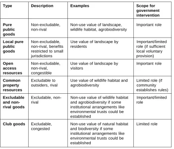
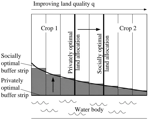
(32) Table 1. Types of public goods (based on OECD 2001a). Type. Description. Examples. Scope for government intervention. Pure public goods. Non-excludable, non-rival. Non-use value of landscape, wildlife habitat, agrobiodiversity. Important role. Local pure public goods. Non-excludable, non-rival, benefits restricted to small jurisdictions. Use value of landscape by residents. Important/limited role (if sufficient local voluntary provision). Open access resources. Non-excludable, non-rival, congestible. Use value of landscape by visitors. Important role. Common property resources. Excludable to outsiders, rival. Use value of wildlife habitat and agrobiodiversity. Limited role (if community establishes rules). Excludable and nonrival goods. Excludable, nonrival. Non-use value of wildlife habitat and agrobiodiversity if some institutional arrangements like environmental trusts could be established. Important/limited role. Club goods. Excludable, congested. Non-use value of natural habitat and biodiversity if some institutional arrangements like environmental trusts could be established. Limited role. However, according to the OECD (2001a), a more detailed classification of public goods (see Table 1) is required in order to arrive at best policy choices. Pure public goods and open access resources are difficult to provide optimally without government intervention, but for other types of public goods the scope for government intervention may be more limited. In the light of the above discussion, let us briefly examine the non-commodity outputs that are selected for analysis in Chapters 3 to 5. Nutrient runoffs from arable lands represent a negative externality which constitutes a market failure as the private and social costs of commodity production diverge and, due to impairments in surface water quality, the value of the public good decreases. Land allocation between alternative crops and linear landscape elements, such as field boundaries and buffer strips, determine the landscape mosaic, and thus the aesthetic and ecological values of landscape, which are public goods. The effects of land allocation on these values are external to the commodity markets, resulting in a divergence between the private and social optima, and thus they constitute a market failure. The agrochemical load from farming affects wildlife habitats adjacent to arable lands and thus agrobiodiversity. Again, an 31.

No results found