Fuzzy modelling and robust control with applications to robotic manipulators

(1)

CONTROL WITH APPLICATIONS

TO ROBOTIC MANIPULATORS

FEI ME!

B. Sc:, Nanjing University, P. R. China

M. Sc., Nanjing University, P. R. China

A thesis submitted for the degree of Doctor of Philosophy

at The University of Tasmania

School of Engineering

Faculty of Science and Engineering

The University of Tasmania

Hobart, Tasmania 7001

Australia

(2)

(3)

The work contained in this PhD thesis is original, to the best of my knowledge and belief, except as acknowledged in the text. This thesis contains no material which has been accepted for the award of any other degree or diploma in any tertiary institution.

Fei Mei

(4)

(5)

In this thesis, fuzzy modelling of a class of nonlinear systems has been investigated based on fuzzy logic and linear feedback control theory, and a few robust variable structure control schemes for nonlinear systems have been developed. A number of robustness and convergence results with dramatically reduced control chattering are presented for variable structure control systems with applications to robotic manipulators in the presence of parameter variations and external disturbances. The major outcomes of the work described in this thesis are summarised as follows.

A robust tracking control scheme is proposed for a class of nonlinear systems with fuzzy model. It is shown that a nominal system model for a nonlinear system is established by fuzzy synthesis of a set of linearised local subsystems, where the conventional linear feedback control technique is used to design a feedback controller for the fuzzy nominal system. A variable structure compensator is then designed to eliminate the effects of the approximation error and system uncertainties. Strong robustness with respect to large system uncertainties and asymptotic convergence of the output tracking error are obtained.

A sliding mode control scheme using fuzzy logic and Lyapunov stability theory has been proposed. It is shown that a sliding mode is first designed to describe the desired system dynamics for the controlled system. A set of fuzzy rules are then used to adjust the controller's parameters based on the Lyapunov function and its time derivative. The desired system dynamics are then obtained in the sliding mode. The sliding mode controllers with fuzzy tuning algorithm show the advantage of reducing the chattering of the control signals, compared with the conventional sliding mode controllers.

A robust continuous sliding mode control scheme for linear systems with uncertainties has been presented. The controller consists of three components: equivalent control, continuous reaching mode control and robust control. It retains the positive properties of sliding mode control but without the disadvantage of control chattering. The

(6)

A robust adaptive sliding mode control scheme with fuzzy tuning has been presented. It is shown that an adaptive sliding mode control is first designed to learn the system parameters with bounded system uncertainties and external disturbances. A set of fuzzy rules are then used to adjust the controller's uncertainty bound based on the Lyapunov function and its time derivative. The robust adaptive sliding mode controller with fuzzy tuning algorithm show the advantage of reducing the chattering and the amplitude of the control signals, compared with the adaptive sliding mode controller without fuzzy tuning. Experimental example for a five-bar robot arm is given in support of the proposed control scheme.

(7)

1. Fei Mei, Man Zhihong, Yu Xinghuo, Thong Nguyen, "A Robust Tracking Control Scheme for a Class of Nonlinear Systems with Fuzzy Nominal Model", International Journal of Applied Mathematics and Computer Science, vol.8, No.1, pp.145-158, 1998.

2. Fei Mei, Man Zhihong, Thong Nguyen, "Fuzzy Modelling and Tracking Control of Robotic Manipulators", to appear in Mathematical and Computer Modelling, 1999.

3. Fei Mei, Man Zhihong, Xinghuo Yu, "Robust adaptive sliding mode control of robots", submitted to IEEE Transactions on Industrial Electronics, 1999. 4. Xinghuo Yu, Man Zhihong, S S Cong, Fei Mei, "Robust adaptive sliding mode

control of robotic manipulators", International Journal of Robotics and Automation, vol.14, no.2, pp. 54-60, 1999.

5. Fei Mei, Man Zhihong, "A Sliding Mode Control System with Fuzzy Logic Controller", International Conference on Computational Intelligence and Multimedia Applications, 9-11 February, 1998, Monash University, Australia. 6. Fei Mei, Man Zhihong, "Fuzzy Modelling and Tracking Control of Nonlinear

Systems", International Congress on Modelling and Simulation Proceedings, pp. 902-906, 7-12 December, 1997, Hobart, Australia.

7. Fei Mei, Man Zhihong, Thong Nguyen, "Continuous sliding mode control with limited control input", Proceedings of the Australian Universities Power Engineering Conference (AUPEC'98), Hobart, Australia, vol.1, pp212-216, September, 1998.

8. Fei Mei, Man Zhihong, Thong Nguyen, "The terminal controller design with application to robotic manipulators", Proceedings of the Australian Universities Power Engineering Conference (AUPEC'98), Hobart, Australia, vol.2, pp532-536, September, 1998.

9. Fei Mei, Michael Negnevitsky, "A robust continuous sliding mode control scheme", Proceedings of 6" International Conference on Fuzzy Theory and Technology, Durham, USA, vol.', pp292-294, October 23-28, 1998.

(8)

Automatic Control (IFAC'99), Beijing, China, vol. H, pp. 349-353, July 5-9, 1999.

11. Man Zhihong, Fei Mei, "A sliding mode control for nonlinear SISO systems with a new fuzzy model", Proceedings of the 14" World Congress of International Federation of Automatic Control (IFAC99), Beijing, China, vol. Q, pp. 359-362, July 5-9, 1999.

12. Fei Mei, Man Zhihong, Xinghuo Yu, Wei Lai, "RBF network based sliding mode control of robots", Proceedings of the IEEE Hong Kong Symposium on Robotics and Control, Hong Kong, vol. 1, pp.27-32, July 2-3, 1999.

(9)

Chapter 1 Introduction

1.1 Motivation

The basis for control system design and stability analysis is a dynamic mathematical model that captures prominent features of the system under consideration. However, in practical situations, such a requirement is not feasible because the controlled systems have high nonlinearities and uncertain dynamics, and simple linear or nonlinear differential equations cannot sufficiently represent the corresponding practical systems, and therefore, the designed controller based on such a model cannot guarantee the good performance such as stability and robustness.

(14)

Many kinds of fuzzy models for control processes have been developed since Mamdani's (1974) paper was published. They can be classified into three kinds of models, Composition Rule of Inference (Zaheh, 1973), Approximate Reasoning Model (Nakanishi et al., 1993), Sugeno's Models such as Position type Model and Position-Gradient type Model (Sugeno and Yasukawa, 1993). Most of these models are expressed by a set of fuzzy linguistic propositions which are derived from the experience of skilled operators or by fuzzy implication which locally represent linear input-output relations of the system.

Most proposed conventional fuzzy models only consider the external behaviour of the system, and can be considered as a function approximation. It is very difficult to obtain a controller using those models. Even if the controller can be obtained by using some trial-and-error procedures the behaviour of the closed-loop system, for example, the stability of the system is still difficult to analyse. Also the number of rules increase very quickly when the system becomes complex because every local rule is only described by a constant. Therefore, the identification of these fuzzy models is still a difficult problem because there are too many parameters in the membership functions.

(15)

Two major conventional control methodologies have been developed for dealing with system uncertainties: adaptive control and robust control. Adaptive control is a control scheme in which so-called adaptation laws are constructed to learn explicitly unknown constant parameters of the system under control. For this reason, adaptive control is limited to those systems whose uncertainties are structured, although it is applicable to a wider range of uncertainties after employing robustness enhancement techniques. Robust control is a control of fixed structure that guarantees stability and performance for uncertain systems. Its design only requires some knowledge about bounding functions on the greatest possible value of the uncertainties. This implies that robust control is capable of compensating for both structured and unstructured uncertainties.

Variable structure control with sliding mode is a robust control technique with respect to system variations and external disturbances. Variable structure control was pioneered in the former Soviet Union in the 1960s by Emelyanov (1962, 1966) and then developed by many researchers (Uticin, 1971, 1977, 1978, 1983; Itks, 1976; Young, 1978, 1988; Slotine and Sastry, 1983; Gao and Hung , 1993). However, the control technique has not been widely accepted in the practical control engineering community, due mainly to the worry of chattering which is inherent in the variable structure control system.

(16)

of complex systems) and conventional linear or nonlinear control theory be combined to improve the system performance and control quality?". The aim of this thesis is to show that by considering both these areas, superior system performance and control quality can be achieved.

1.2 Scope

The aim of this thesis is to present new robust control schemes by incorporating artificial intelligent techniques such as fuzzy logic and neural networks with conventional variable structure control system. In line with this, a review of basic variable structure control theory and discussion of recent research results on the robust variable structure control for a class of nonlinear systems with uncertain dynamics is given.

Fuzzy logic and fuzzy logic control are also reviewed to present a background to the methodology to be employed. Fuzzy sets, fuzzy reasoning, and fuzzy controller design are described.

(17)

1.3 Thesis outline

The thesis is organised as follows.

In Chapter 1, the major thrust of the thesis, the motivation, scope and thesis outline are introduced.

In Chapter 2, the basic theory of variable structure control systems is briefly surveyed. Because the variable structure theory has many good features, it can be easily used to design controllers for linear or nonlinear systems. Although the robustness can be achieved without the exact knowledge of the control system, the system performance and control quality depend very much on the choosing of sliding mode parameters and the estimating of bounding functions of the system's unknown parts. In practice, excessive control input and severe control chattering which may excite unmodelled high-frequency dynamics are highly undesirable. In the following chapters of this thesis, several new and improved robust variable structure control schemes of nonlinear systems will be proposed by combining conventional methods and recently developed techniques, namely fuzzy logic and neural networks, and it will be shown to improve the system performance and enhance the control quality.

(18)

defuzzifier. Commonly-used kinds of membership functions are described, focusing on control applications. The prominent advantage of the fuzzy logic controller is that it can effectively control complex ill-defined systems having nonlinearities, parameter variations and disturbances. However, there also exist some impediments in the design of the fuzzy logic controller. In general, fuzzy rules are obtained on the basis of intuition and experience, and membership functions are selected by trial and error procedure. Moreover, it is not easy to mathematically prove the system stability and robustness due to linguistic expression of the fuzzy rules. Therefore, a systematic design method of the fuzzy logic controller from which the stability and robustness can be clearly seen is to be explored (Lee, 1990). The succeeding chapters will employ fuzzy logic to establish system model of a class of nonlinear systems and enhance robustness and control quality of variable structure control systems.

In Chapter 4, a robust tracking control scheme is proposed for a class of nonlinear systems. The main contribution of this scheme is that a nominal system model for a nonlinear system is established by fuzzy synthesis of a set of linearised local subsystems, where the conventional linear feedback control technique is used to design a feedback controller for the fuzzy nominal system. A variable structure compensator is then designed to eliminate the effects of the approximation error and system uncertainties. Strong robustness with respect to large system uncertainties and asymptotic convergence of the output tracking error are obtained. A simulation example is given to support the proposed control scheme.

(19)

first designed to describe the desired system dynamics for the controlled system. A set of fuzzy rules are then used to adjust the controller's parameters based on the Lyapunov function and its time derivative. The desired system dynamics are then obtained in the sliding mode. The sliding mode controllers with fuzzy tuning algorithm show the advantage of reducing the chattering of the control signals, compared with the conventional sliding mode controllers. The fuzzy tuning algorithm is also applied to the adaptive sliding mode control. Simulation and experimental examples are given in support of the proposed control scheme.

In Chapter 6, a robust continuous sliding mode control scheme for linear systems with uncertainties is developed. The controller consists of three components: equivalent control, continuous reaching mode control and robust control. It retains the positive properties of sliding mode control but reduces the disadvantage of control chattering. The proposed control scheme is applied to the tracking control of a one-link robotic manipulator by fuzzy modelling of the nonlinear system.

(20)

tuning. Experimental example for a five-bar robot arm is given in support of the proposed control scheme.

In Chapter 8, a new adaptive sliding mode controller is developed for trajectory tracking of robotic manipulators. This controller is able to estimate the constant part of the system parameters as well as adaptively learn the uncertain part of the system parameters by the Gaussian neural network. It is shown that under a mild assumption, the proposed control law does not require measurement of acceleration signals. This new control law exhibits the good properties as shown in Slotine and Li (1987) and keeps the chattering to a minimum level. An experiment for a five bar robotic system is carried out to confirm the effectiveness of the approach.

Chapter 9 summarises the results and draws conclusions. A brief review of each chapter is given, noting the important results. Topics and aspects for future work are suggested.

Appendix

(21)

Chapter 2 A Survey of The Variable Structure

Control Theory

2.1 Introduction

We have mentioned in chapter one that the variable structure control theory is a robust control with respect to system uncertainties and external disturbances. Generally speaking, variable structure control can be considered to be an extension of conventional feedback control in the sense that the structure of a state feedback regulator is allowed to change as its states cross discontinuity surfaces, which results in discontinuous feedback control input on one or more manifolds in the state space. From the point of the conventional feedback control theory, a variable structure control system can be treated as a combination of subsystems. Each subsystem has a fixed structure and operates in a specified region of the state space. The combination of these subsystems according to some prescribed rules results in a new system which is different from the individual subsystems and has the desired system response.

(22)

switching planes forms a sliding mode. The purpose of the variable structure controller is to drive the system states into the sliding mode on which the sliding motion occurs and the motion of the system is thus formally equivalent to a system of low order, called as equivalent system. Actually, the sliding motion on the sliding mode is the convergence motion of the system states from arbitrary initial values to the origin. The convergence rate depends on the design of sliding mode parameters. It is due to this feature that the variable structure control is also called sliding mode

control.

Another feature of a variable structure system is that the transient response can be divided into two parts. First, the motion in which the variable structure controller drives the switching plane variables to reach the sliding mode. Second, the sliding motion in which the system states constrained on the sliding mode asymptotically converge to the origin. Usually, the sliding motion is determined only by the sliding mode parameters. However, the convergence of the switching plane variables are affected by the sliding mode parameters because the sliding mode parameters are involved in the controller gain matrices.

In this chapter, we will first review the basic variable structure control theory that has been useful in establishing robust variable structure control algorithms. In view of the focus of the thesis, we will then restrict our discussion to recent research results on the robust variable structure control for a class of nonlinear systems with uncertain dynamics.

(23)

2.4, a robust variable structure controller design using reaching law method has been presented for robot manipulators.

2.2 Basic variable structure control theory

2.2.1 System model and sliding mode

Consider the following linear time invariant system

X(t) = A X(t) + B u(t) (2.1)

where X E Rn and u E Rm represent the state and control vectors, A e Rnxn and B E

Rnxm _{are constant system matrices. It is assumed that n > m, B is of full rank m, and} the pair (A, B) is completely controllable.

Define a set of switching plane variables si (i = 1 m) passing through the state space

origin

s. = C. X i = 1 m (2.2-a)

or S = C X (2.2-b)

R

where • e n is a constant vector and

C = [ C I ... CTm (2.2-c)

is an nxm constant matrix.

System (2.1) is said to attain a sliding mode when the state vector X reaches and remains on the intersection (S = 0) of the m switching plane variables

=

S₀_{= s = X: C. X 0, i = 1 ... m} 1

=

1

(24)

The control input vector u(t) in the variable structure control system usually has the following form (Utkin, 1977)

u(t) = K X + w X (2.4)

where the first term in expression (2.4) is a linear feedback and the second term is a switching component. w = [ wij 1 and

11/ —

ía

M./

s i xj < 0

s i x j > 0 (2.5)

The task of the control input u(t) in expression (2.4) is to drive the switching plane variables to reach the sliding mode (2.3) by the suitable design of the controller gain matrices K and w. Thereafter, the system performance will be determined by the sliding motion on the sliding mode. Generally, the sliding mode is designed such that the system response restricted on the sliding mode has a desired behaviour such as asymptotic stability and prescribed transient response. Usually, the switching plane variables are designed as a linear functions of the system states. Many researches have shown that it is convenient for the linear sliding mode to be used in the design and analysis for a variable structure control system.

The next important problem is how to design controller parameters to guarantee the switching plane variables to reach the sliding mode, and then remain on the sliding mode. The work in Utkin (1977, 1978) and Young (1982) have shown that if the control input u(t) is designed such that the tangent vector or time derivative of the switching plane variables always point toward the sliding mode surfaces, then the switching plane variables s i (i = 1, m) asymptotically converge to zero, and the

system states can remain on the sliding mode.

(25)

1 V = —

2 S T

S (2.6)

In this case, the sufficient condition for the switching plane variables to reach the sliding mode surfaces can be expressed as follows

•

STS < 0 (2.7-a)

or

S. S. < 0 _I

(i = 1, m) (2.7-b)

It has been noted that most of the variable structure control algorithms are designed based on the sufficient condition in expression (2.7-a) or expression (2.7-b) (Utkin, 1978 and DeCarlo, 1988).

2.2.2 Equivalent control

On the sliding mode, s = 0 and = 0 (i = 1, ...m). Then, using expressions (2.1) and (2.2), we have

= CAX + CBu_eq= 0 (2.8)

where u_eqis called as equivalent control.

If IC 1131# 0, the equivalent control u_eqcan be written as

ueq = -(CB) 1 CAX

=-KX (2.9-a)

(26)

The system response on the sliding mode can then be described by the following differential equation

X(t) = A X(t) - B(C B) AX(t)

= [ I - B(CB)-1C A X(t) (2.10)

System (2.10) is called equivalent system. The characteristics of the equivalent system (2.10) can be summarised as:

(1) The dynamical behaviour of the equivalent system is independent of the control input and depends only on the choice of the matrix C in expression (2.2-c). Therefore, the control input is just used to drive the system states into the sliding mode and thereafter to maintain it on the sliding mode. The determination of the matrix C may thus be completed with no prior knowledge of the form of the control input.

The reason for the equivalent system to have an independent motion from the control input is due to the fact that the matrix CB is nonsingular. In fact, the condition ICBI#0 means that the null space of C and the range space B are complementary subspaces. Thus, when the sliding motion occurs on the sliding mode or within N(C), the behaviour of the equivalent system is unaffected by the control input. If 'CBI.° as shown in Utkin (1977), the equivalent control is either not unique or does not exist. Therefore, sliding mode can not be reached.

(2) Equivalent system (2.10) is an (n-m)th order system. The work in Darling and Zinober (1986) has shown that for the matrix B with full rank m, there exists an orthogonal nxn transformation matrix T such that

(27)

CHAPTER 2 A SURVEY OF VARIABLE STRUCTURE CONTROL 15

where B 2 is an mxm nonsingular matrix.

Define a transformed state variable vector Y = T X, state equation (2.1) becomes

ir = TATT Y + TBu (2.12)

If Y is partitioned as

yT = i vT yT 1

L '1 '2 i

and matrices T A TT and CTT are partitioned as

TAT T =[ A "

A 21 A Al2

22

1

C TT = [c1 c2 _]

then, the system (2.12) can be written in the following form

Y = AYI + A1 1 2 Y2

Y2 = AY1 + A2 2 Y2 -I- B2 U

On the sliding mode, we have C l Y1 + C2 Y2 = 0 Or

Y₂ = - _{F Y1} where

F = C-1 _{2 1} C

(2.13-a)

(2.13-b)

(2.13-c)

(2.14-a)

(2.14-b)

(2.15-a)

(2.15-b)

(28)

The equivalent system can then be written in the following form

= (Ai - Al2 F) Y1 (2.16)

Therefore, we can see from expression (2.16) that the equivalent system is (n-m)th order system, i.e., the system dynamics is simplified on the sliding mode.

2.2.3 Robustness property

Robustness property is an important feature of a variable structure control system. Suppose that system (2.1) has uncertainty in matrix A and external disturbance, then the system state equation can be written in the following form

X(t) = (A0 + AA) X(t) + Bu + Df (2.17)

where A₀ is the nominal system matrix, AA is the uncertainty, f E RL is a bounded external disturbance vector, and matrix D is compatibly dimensioned. Without loss of generality, it can be assumed that matrices B and D are full rank and the uncertainty presented in the input distribution matrix B is incorporated in the system disturbance term. During the sliding motion, the state vector of the system satisfies the following equations

C X = 0 (2.18-a)

C(A + AA)X + CBueq + CDf = 0 (2.18-b)

From expression (2.18-b), the equivalent control can be achieved as

u_{eq = - (}CB )-1 C ( AX + AAX + Df ) (2.19)

(29)

= [ I - B( CB )-IC AX + AAX + Df ) (2.20-a)

CX = 0 (2.20-b)

Spurgeon (1991) has shown that the sliding mode system (2.20) is insensitive to parameter variations and the external disturbance if and only if the system uncertainty AA, matrices B and D satisfy the following rank relation

rank [ B : DI = rank [ B : AAT] = rank [B] (2.21)

where T is the matrix of the basis vectors of the reduced-order sliding subspace defined by expression (2.20).

Expression (2.21) is also called as the invariance condition. In addition, the robustness property for variable structure systems have been investigated by other researchers. For example, Gutman (1979) and Bormish and Leitmann (1983) have shown that if system uncertainties and disturbance satisfy the "matching condition", then the system is completely insensitive on the sliding mode, and the effect of disturbance and parameter variations can be minimised by minimising the time required to attain the sliding mode.

2.2.4 Two methods of sliding mode design

(30)

The quadratic minimisation method for the sliding mode design was proposed by Utkin and Young (1978). In this method, the following cost function is defined

J(u) = X(OTQX(t)dt (2.22)

where Q is a symmetric positive-definite matrix, and t s denotes the time at which the

sliding mode starts.

Partitioning the following matrix compatibly with Y (see subsection 2.2.2)

TTQT =[ QH

where matrix T is defined

the cost function (2.22)

1

J(v) = — 2

ts

where

Q* = _{Q 1 1}

A* = A 11

v(t) = Y₂

Y₁ = A*Y

Q21 Q12 Q22 in can then 00 f

YT_{I Q}*

- Q _{12 22%1}

-0 _iz_--₂₁₂

+ Q-1 Q₂₂ ₂₁

1 + A12

expression (2.11),

be expressed in the following form

Y I + vTQ₂₂V }dt

0 _—21

Y ₁

V(t) (2.23) (2.24) (2.25-a) (2.25-b) (2.25-c) (2.25-d)

(31)

v(t) = - _Q-212ATI2PYI

Using expression (2.25-e) in expression (2.25-c), we have

(.1_1 r n AT 0, i v

Y2 = - '22 1- '21 + '12 1 J i l = - FYI

where the matrix P satisfies the following Riccati equation

-1 n

PQ* + A*_{P -}_PA_l2(1 AT₂₂_1-_'1210, _{± `:}_{= '}n

and matrix

-I r T 1

F = (222 1- Q2I + A l2 P -I

(2.25-e)

(2.26)

(2.27-a)

(2.27-b)

can then be determined as required.

The eigenstructure assignment method is also very popular in the sliding mode designs and it was first used by Utkin and Young in 1978.

Suppose that the sliding mode has commenced on N(C). Then the equivalent system can be written as

X(t) = (A - BK)X(t)

where matrix K is given in expression (2.9-b).

During the sliding motion, the state variables must remain in N(C) so that

C[ A - BK ] = 0 <=> R(A - BK) c N(C)

(2.28)

(2.29)

Let Xi (i = 1, ... n) be the eigenvalues of A - BK with corresponding eigenvectors vi,

(32)

C[ A - BK lv i = X.Cv. = 0 _(2.30)

Expression (2.30) shows that either X i is zero or v i E N(C). Since A - BK = A eg has m zero-valued eigenvalues, we can set { X i : i = 1, n-m } be the nonzero eigenvalues and therefore, specifying the corresponding eigenvalues { v i : i = 1, n-m } fix the

null space of C (dim[N(C)] = n - m).

It is noted that C is not uniquely determined because the equation

CV = 0, V = [v 1 vn _m

(2.31)

has m2 degree of freedom, which may be easily seen if we define

W = [ 1= Tv (2.32)

W2

where the partitioning of W is compatible with that of Y, then expression (2.31) becomes

0 = CTT. Tv = [C I C2 ] [

W 21= C 2 ( F

—

[ W1 1 W2

Therefore, F can be determined from the following equation

FW 1 = - W2

(2.33)

(2.34)

(33)

Some other eigenvector assignment methods have also been proposed, and the details can be found in Moore (1976), Klein and Moore (1977) and Sinswat and Fallside (1977).

2.2.5 Controller designs

In most of the variable structure control schemes, the control law usually consists of a NL

linear component uL and a nonlinear component u which are assumed to form control input u. The linear part is merely a state feedback

= KX (2.35)

While the nonlinear signal incorporates the discontinuous elements of the control. Some examples of possible types of nonlinearity are as given below.

(a) A nonlinear component with constant gains

NL

ui = Misgn( CiX), M1 > 0

(b) A nonlinear component with state-dependent gains

NL

M

U. = i(X) sgn( C X ) mi(.) > 0

(2.36)

(2.37)

(c) A linear feedback with switching gains

u

NL

= TX

(2.38-a)

(34)

(d)

j =

A unit

NEL

•

sl

< 0 s_ix

>

0

vector nonlinearity with scale factor

NX

(2.38-b)

(2.39)

Ilmx11

where the null spaces of N, M and C are coincident.

The nonlinear control component is discontinuous on the individual hyperplane in cases (a) - (c). This may result in wasted control effort as the system state pierces one hyperplane, and is forced into another surface. In case (d), the individual controls are continuous, except on the intersection of the switching plane variables where all the nonlinear control elements become discontinuous together. The details of cases (a) - (d) are shown in Uticin (1978), Ryan (1983), Young (1977) and Dorling and Zinober (1983). Some special properties and behaviours of a system with control type (d) has been discussed in Surgeon (1991).

2.3 Variable structure control of nonlinear system

2.3.1 System model

In section (2.2) we have briefly reviewed the basic variable structure control theory of linear systems. Most of these ideas can be extended to the variable structure control of nonlinear systems. However, the complexity of the analysis and the controller designs may be increased due to the nonlineatity in the nonlinear system model. From the engineering point of view, the following nonlinear system is often considered (DeCarlo, et al., 1988).

(35)

where the state vector X(t)E Rn, the control input vector u(t) E Rm, f(t, X) E Rn and B(t, X) E Rnxm. Further, each entry in f(t, X) and B(t, X) is assumed to be continuous with continuous bounded derivative with respect to X.

Each entry u(t) of the control input vector has the following form

(t, X) u ; (t, X) = '

u (t, X)

with cri (X) > 0

with a; (X) <0 (2.41)

whereis the ith switching ,surface associated with the (n-m) dimensional _a_t_(x) switching surfaces

a(X) = [al (X), , szYm(X)

2.3.2 Sliding mode and equivalent control

Following the sliding mode design for linear systems in section 2.2.4, the method of equivalent control is a way to determine the system motion restricted tO the sliding mode a(X) = 0. Suppose that there exists a time to > 0, and the state of the system reaches the sliding mode after t to. On the sliding mode, the following two equations are satisfied

cr(X(t)) = 0 t to

a(X(t)) =0 t to

Using system equation (2.40), expression (2.43-b) can be expressed as follows

(2.43-a) (2.43-b)

acy(x),

f(t, X) + B(t, X)ueq =

o

ax

(2.44)

(36)

where u_eqis the so called equivalent control which can be obtained from expression (2.44) as follows

-1

au(X)

aa(x)

U = -

- ti(t, X) - f(t, X)

eq

r

OX

,

_ax

(2.45)

Using expression (2.45) in system model (2.40), the dynamics of the closed loop system on the sliding mode is given by

-1 acs(X)

[ - B(t, X)( a(X)B( X)) f(t, X)

_ax

ax

(2.46)

Therefore, the problem of the sliding mode design is to choose the parameters in a(X) = 0 such that the equivalent system (2.46) is stable. In most of variable structure control schemes for nonlinear systems, the linear sliding modes are often used. Therefore, some methods of sliding mode design in sections 2.2.4 can also be used.

2.3.3 Controller design

2.3.3.1 Diagonalisation method

In general, for nonlinear system equation (2.40), the control input is an m dimensional vector and each entry has the structure of the form

u!," (t, X)

u = _

u (t, X)

for a, (X) > 0

for

a

-

,

(X) < 0 (2.47)

To determine the switched feedback gains in control law (2.47), the following diagonalisation method is often used (DeCarlo et al., 1988).

(37)

1 r

aci ,

u(t) =*

Q .` (t, X) I_ - 113(t, X)u(t)

.(x)

ax

(2.48)

where Q-1(t, X)(aa/aX)B(t, X) is a nonsingular transformation, and Q(t, X) is an arbitrary mxm diagonal matrix with elements q i (t, X) (i = 1, m) such that inflqi (t, X)I > 0.

Using expression (2.48) in expression (2.40), the system dynamics becomes

= f(t, X) + B(t, X)1_ r aa(X)B(t, X) -1Q(t, X)u * (t) ax

If u * is selected such that

qi (t, X) u *: < - V o(X) f(t, X) ai (X) > 0

qi (t, X) u *i > - Vai (X) f(t, X) ai (X) < 0

(2.49)

(2.50-a)

(2.50-b)

then,

T(X)ã(X) <0 (2.51)

Expression (2.51) is the reaching condition for the system states to reach the sliding mode surfaces a(X) = 0. On the sliding mode, the desired system dynamics can be obtained. Also, the control input u(t) can be obtained from equation (2.48).

2.3.3.2 Reaching law method

(38)

stable a(X) is itself a reaching condition, i.e. aT(X)d(X) <0. In addition, by choice of the parameters in the differential equation, the dynamic quality of VSC system in the reaching mode can be controlled. A practical general form of the reaching law is

= —Q sgn(a) — Kh(a) (2.52)

where

Q = diag[q,,• • •,q], q, > 0 sgn(a) = [sgn(a,),• • •,sgn(am

K = diag[lc,,• • •, k], k, > 0 h(a) = [hi(a1),•••,hm(a.)Ir

1h1( 1)> O, h1(0)=

Three practical special cases of (2.52) are given below. 1) Constant rate reaching

= Q sgn(a) (2.53)

This law forces the switching variable a(X) to reach the sliding mode surfaces a(X)=0 at a constant rate = —q1. The merit of this reaching law is its simplicity. But, if q. too small, the reaching time will be too long. On the other hand, a q, too large will cause severe chattering. In the following chapters of this thesis, a fuzzy tuning algorithm for q, will be introduced to optimise the system performance.

2) Constant plus proportional rate reaching

= —Q sgn(a) — Ka (2.54)

(39)

1 kla. 1+q, T = ln "° .

k1 q1

3) Power rate reaching

6 = —1c1lada sgn(61), 0< a <1,i =1,...,m (2.55)

This power rate reaching law increases the reaching speed when the state is far away from the sliding mode surfaces a(X)=0, but reduces the rate when the state is near the surfaces. The result is a fast reaching and low chattering reaching mode. Integrating (2.55) from a, = c a, = 0 yields

1

T, = la I 1 - Wki (

a), i = 1, m (2.56)

showing that the reaching time is finite.

The control law can be determined by the time derivative of a and the reaching law (2.52), i.e.,

u =acY

aX B(t X)1-1

r a

' f(t, X) + Q sgn(a) + Kh(a)1 j

Lax

-1

where the matrix [-a-CY is nonsingular.

Lax

(2.57)

2.3.4 Robust control of nonlinear systems

In practical situations, the system dynamics of a nonlinear system is different from its nominal system model due to parameter uncertainties. To represent parameter uncertainties in the plant, the following state equation is considered (DeCarlo, 1988).

= [ f(t, X) + Af(t, X, r(t)) _I + [ B(t, X) + B(t, X, r(t)) 11(0 (2.58-a)

(40)

In most of researches (Corless and Leitmann, 1981; Gutman and Palmor, 1982; Peterson, 1985), the plant uncertainties Af and AB are assumed to lie in the image of B(t, X) for all variables t and X (this is called "matching condition'). Then dynamic equation (2.58-a) can be expressed as follows

= f(t, X) + B(t, X)u + B(t, X)e(t, X, r, u) (2.58-b)

where e(t, X, r, u) represents system uncertainties.

DeCarlo et al. (1988) shows that if e(t, X, r, u) is bounded by a positive function p(t)

II e(t, X, r, u)11 2 p(t) (2.59)

and control input has the following form

where

U = U_eq +u

n

u

eq = _ [ B(t, X) 1 -1 a

[ cy

at

(X) ±

a

(x

)

)f(t,

x)

ax

BT(t, X) V x V(t, X) A

U_n — - T

2

p(t x)

II

B .(t, X) V,V(t, X) I I

(2.60-a)

(2.60-b)

(2.60-c)

A

p( t, X) = a + p(t, X)

(2.60-d)

[ a6(t, X) ]T

VxV(t, X) =

a(t, x)

ax

(2.60-e)

(41)

The results discussed in this section forms the foundation of the variable structure control theory for nonlinear systems. Although there are many classes of nonlinear systems, robustness and convergence of variable structure control systems may be established based on the results in this section (Utkin, 1978; Young, 1978 and DeCarlo et al., 1988).

2.4 Application to robot manipulators

A robotic manipulator is a typical nonlinear system. The investigations for the control of robotic manipulators have not only improved the robotic system performance, but also developed many new control techniques which have enhanced the modern control theory. Many control schemes such as feedback control and adaptive control have been developed for robotic manipulators. However, the variable structure control technique is one of the most powerful techniques due to the fact that the variable structure control can deal with systems with large uncertainties, bounded disturbances and nonlinearities. In recent years, the designs of robust variable structure control laws for rigid robotic manipulators that ensure robustness and asymptotic trajectory tracking have been investigated by many researchers. Many robustness and convergence results have been obtained by Young (1978, 1988), Morgan and Ozguner (1985), Slotine and Sastry (1983), Yeung (1988) and Leung et al (1991). In this section, the dynamics of the robotic manipulator and a robust variable structure controller design using the reaching law method (Gao and Hung, 1993) will be presented to highlight the main issues of the control scheme.

2.4.1 Dynamics of robotic manipulators

(42)

dkj(q) + fijk(q) + (q) = Tic k = 1, n (2.61)

where dk. are the coefficients of the inertia matrix D(q), k(q) are the gravitational forces and Tic are the input torques. The coefficients f of the coriolis and centrifugal terms are defined as

ad

ki

ad,„ ad

ii

}

a

q;

a

q;

a

q

k

1

fijk = (2.62)

and f are known as Christoffel symbols.

It is common to write expression (2.62) in matrix form as

D(q) + F(q,

4 +

G(q) '= (2.63)

where the k,jth element of the matrix F is defined as

n AA

ad.. .

f = I _adki

_

)(11

kJ 2k. -_,

i=1 o_qi_a_qi_a_qk

(2.64)

and the component of G(q) is Ok.

Although the equation of motion (2.63) is complex and nonlinear for all but simple robotic manipulators, it has several fundamental properties which can be exploited to facilitate control system design (Ortega and Spong, 1989).

Property 1: The inertia matrix D(q) is symmetric, positive-definite, and both D(q) and D(q)4 are uniformly bounded as a function of q.

Property 2: There is an independent control input for each degree of freedom.

(43)

generalised coordinates. By defining each coefficient or a linear combination of them as a separate parameter, a linear relationship results so that we may write equation (2.63) as

D(q)

4 +

F(q, q)

4 +

G(q) = Y(q, q,

4)o =

(2.65)

where Y is an nxr matrix of known functions, known as the regressor, and q is a n dimensional vector of unknown parameters as shown in Spong and Vidyasagar (1989).

It can be seen later that the manipulator system (2.63) can also be expressed into the generalised form in expression (2.40). Therefore, the basic variable structure theory can be used to design robust controllers and the structural properties mentioned in the above can then be used to simplify controller designs.

2.4.2 A robust VSC controller design

Consider an n-link manipulator system with perturbations and disturbances described by

D(q)4 + F(q, q)q + G(q) = w(q, q, p, t) (2.66)

where p is an uncertain parameter vector, w(q,q, p, t) is the collection of all system perturbations and external disturbances. The state variable is defined as

X = {q T T (2.67)

Then (2.66) can be put into the form

X = f(t, X) + B(t, X)u + v(X, p, t) (2.68)

where

U = T,

0 v(X, p, t) = [

(44)

f(t, X) =

(q)(F(q, q)q + G(q))1B' (t X) = [ (q)].

The arm is to track a desired motion Cld (t). The output tracking error is defined as

= d e = [ET •11T _(2.69)

The sliding mode surfaces are chosen as

a(e) = Ce = [A

11[]=

Ac (2.70)

Adopt the reaching law

= sgn(a) Ka

Taking the time derivative of (2.70) gives

(2.71)

eT=At+

=Ae+q d +D-I (Fq+G—w—u) (2.72)

• Equating (2.71) and (2.72) and solving for the control u yields

u = D{Qsgn(a)+ Ka + Ae + qd } + Fq +G — w (2.73)

All quantities on the right-hand side of (2.73) are known except the disturbance w,

which is unknown. To cope with this problem, define

w₁ =1:30-1 w

and assume that w1 is bounded by

(2.74)

(2.75)

Then replace w in (2.73) by —DW sgn(a) give following control law

u = D{Q sgn(a) + Ka + Ae + q d } + Fq + G + DT/ sgn(a)

Substituting (2.76) into (2.72) give

(45)

6 = —Q sgn(a) — Ka — w 1 — sgn(a) (2.77)

Thus, the reaching condition aT6 < 0 is guaranteed.

This robust controller design is based on the bounding function estimation of the system perturbations and external disturbances, and the exact system knowledge is not required. However, the system performance and control quality depend very much on the choice of sliding mode parameter Q and the estimation of bounding function of the unknown parts. Excessive control torques and severe control chattering may be easily caused by over estimation of control parameters.

In order to overcome these shortcomings, in chapter 5 of this thesis, fuzzy logic technology will be used to dynamically adjust the sliding mode parameter Q, and control chattering will be reduced dramatically. In chapter 8, a robust adaptive control scheme for robots is established where neural network has been constructed to adaptively learn the bounding function of the unknown parts of the robot system.

2.5 Concluding remarks

(46)

(47)

Chapter 3 Fuzzy Logic and Fuzzy Logic Control

3.1 Introduction

Zadeh (1965) published his first paper on a novel way of characterising nonprobabilistic uncertainties, which he called "fuzzy sets". Fuzzy logic and fuzzy set theory has now evolved into a fruitful area containing various disciplines, such as calculus of fuzzy if-then rules, fuzzy graphs, fuzzy interpolation, fuzzy topology, fuzzy reasoning, fuzzy inference systems, and fuzzy modelling. The applications, which are multi-disciplinary in nature, include automatic control, consumer electronics, signal processing, time-series prediction, information retrieval, database management, computer vision, data classification, decision-making, and so on.

(48)

explained, is a means of computing with words for which the role model is the human ability to reason and make decisions without the use of numbers (Zaheh, 1996). The first implementation of these ideas was described in a paper by Mamdani (1974). The key principle underlying fuzzy logic control is based on a logical model which represents the thinking process that an operator might go through to control the system manually. The viability of fuzzy logic control has been demonstrated through wide-spread applications (Schwartz et al, 1994). Fuzzy logic control can be considered as one of the intelligent control techniques wherein engineering knowledge is reflected in the controller. It has been found that such controllers have definite advantage over the traditional HD controllers in that they are more robust with respect to structured or unstructured uncertainties. The linguistic characteristics of fuzzy control provide a very good approach to account for the sensor noise, unmodelled dynamics, parameter variations, disturbances and nonlinearities (Lee, 1990).

(49)

chattering is an undesirable disadvantage inherent to conventional sliding mode control.

In recent years, fuzzy modelling of controlled systems has received much attention. A number of researchers (Feng and Cao et al, 1997; Tanaka et al, 1996) proposed fuzzy global systems with stability analysis based on Takagi-Sugeno fuzzy inference model. Mei & Man et al (1998) presented a fuzzy modelling and robust tracking control scheme for a class of nonlinear systems by fuzzifying over a number of operating points within the interested range.

Despite a large number of technical publications focusing on fuzzy systems, there exist some doubtful opinions on fuzzy controllers mainly due to some misunderstanding about fuzzy control. Attempts have been made to clear up this misunderstanding, e.g. Jager (1995). It is, therefore, of interest to start the notable part of this thesis, with a short primer on fuzzy set theory, fuzzy reasoning, and fuzzy logic control, using fuzzy tool in combination with other techniques.

The arrangement of this chapter is as follows. Section 3.2 gives the definitions of fuzzy sets, fuzzy set operations, fuzzy relation and compositions, and linguistic representations. Section 3.3 describes fuzzy logic and fuzzy reasoning. Section 3.4 introduces fuzzy logic control.

3.2 Fuzzy set theory

(50)

applied to engineering problems. The purpose of this section is to briefly summarise the basic concepts that are necessary in understanding fuzzy logic and fuzzy inference from a practical viewpoint.

3.2.1 Fuzzy sets

A universe of discourse (or domain of definition) U is the set of allowable values for a variable, denoted generically by {x} which could be discrete or continuous, where x represents the generic element of U.

A crisp set A in a universe of discourse U can be defined as A = {xi _(x)} where

/AA (x) is, in general, a condition by which x e A. If we introduce a zero-one characteristic function such that A = 02A (x) = 1 if x e A and //A (x)= 0 if x 0 A) then

/L A (X) is called a membership function for A.

A fuzzy set F in a universe of discourse U is characterised by a membership function

kt F (x) which takes on values in the interval [0, 1]. A fuzzy set may be viewed as a

generalisation of the concept of an ordinary (i.e. crisp) set whose membership function only takes two values {0, 1}. A membership function for a fuzzy set F provides

a measure of the degree of similarity of an element in U to F. A fuzzy set F in U may

be represented as a set of ordered pairs of a generic element x and its grade of membership function: F = ((x„ u F (x))1x ctn. When U is continuous, F can be

written concisely as F = fu,uF(x)Ix, where the integral sign denotes the collection of all points x E U with associated membership function I, F (x). When U is discrete, F is

represented as F=

E

t

F

(xxx„

where the summation sign stands for the union of

XiEU

(51)

70 90 100 weight(kg) 40 50

Degree of membership

LIGHT HEAVY

0.5

crossover pclint

0

does not imply division. Note that in fuzzy sets, an element can reside in more than one set to different degrees of similarity. This cannot occur in a crisp set theory.

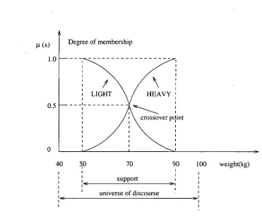
The support of a fuzzy set F is the crisp set of all points x E U such that /.2 F (x)> 0. The element x E U at which ki F (x) = 0.5 is called the crossover point. For example, the formal domain for normal weight might be 40 to 100 kg. However, the fuzzy sets HEAVY and LIGHT can have non-zero membership grade at 50 to 90 kg with a crossover point at 70 kg, as shown in Fig. 3.1. A fuzzy set whose support is a single point x in U with /./ F (x) =1 is referred to as fuzzy singleton. In a singleton output space, fuzzy set membership functions are represented as single vertical points. Figure 3.2 illustrates how a variable SPEED can be composed on individual single points.

support

[image:51.565.81.452.392.699.2]

universe of discourse

(52)

A

1

1 (x)

1

0

■

40 60 80 speed(km1 h) Fig. 3.2 Singleton representation.

3.2.2 Set theoretical operators (Lee, 1990)

Let fuzzy sets A and B in U be described by their membership functions ,u A (x) and 14, B (x). The set theoretic operations of union, intersection and complement for fuzzy sets are defined as following.

Union (disjunction): The membership function R AL,Bof the union A u B (A OR B) is pointwise defined for all x E U by

AuB(x) =max(RA(x), 1u 8 (x)} (3.1)

P

Intersection (conjunction): The membership function _,_L1An/3 of the intersection A n B (A AND B) is pointwise defined for all x E U by

ktiar,B(x)= min{,uA (x), ,u 8 (x)} (3.2) Complement (negation): The membership function R A of the complement of a fuzzy set A, A (NOT A), is pointwise defined for all - X E U by

(53)

10 0.8 0.6 0.4 0.2 0

o 5

(a) 0.8 0.6 - 0.4 - 0.2 - 0 o 1 0.8 0.6 0.4 0.2 0 o 5 (b) 5 (d) 10 10 Fig. 3.3 illustrates these three basic operations: a) illustrates two fuzzy sets A and B,

b) is the complement of A, c) is the union of A and B, and d) is the intersection of A and B.

Fig. 3.3 Operations on fuzzy sets: (a) two fuzzy sets A and B; (b) A; (c) AuB;(d) AnB.

Note that other consistent definitions for fuzzy AND and OR have been proposed in the literature under the names "T-norm" and "T-conorm" operators (Mendel, 1995), respectively.

(54)

mil-0,A,

xY,

max(0, x + y — 1},

x

if y = 1 yif x=1 , 0 if x, y <1

fuzzy intersection algebraic product

bounded product

drastic product

x y =*

where x,

y

E [0,1] .

T-cononn: A t-conorm, denoted by ®, is a two-place function from [0, 1] x [0, 1] to [0, 1], which includes fuzzy union, algebraic sum, bounded sum, and drastic sum, defined as

x@y=

- max{x, y}, fuzzy union

x + y—

xy,

algebraic sum

minfl,

x

+ yl , bounded sum

x

if y = 0

y if

x =

0 drastic sum

‘. lifx,y>0

where

x,

y e [0,1].

3.2.3 The extension principle

The extension principle is a tool for generalising crisp mathematical concepts to fuzzy sets. It has been extensively used in the fuzzy literature.

The extension principle: Let U and V be two universe of discourse and f be a mapping from U to V. For a fuzzy set A in U, the extension principle defines a fuzzy set

B

in V by

(55)

That is, ,u B (y) is the superium of At A (x) for all x E U such that f(x)=y, where y E Vand we assume that f-1(y) is not empty. If f-1(y) is empty for some y E V, define /48(y)=0.

3.2.4 Fuzzy relations and their compositions

Cartesian product: If An are fuzzy sets in , respectively, the Cartesian product of A1,..., An is a fuzzy set in the product space u, x...xu with the membership function

YAI x...xA„ = mintgA, (xn )1 (3.5a)

Or

(xi,. ..,x) = ₍_x,_)...,uAn(xn) (3.5b)

Fuzzy relations: Fuzzy relations represent a degree of presence or absence of association, or interconnection between the elements of two or more fuzzy sets. An n-ary fuzzy relation is a fuzzy set in u,x...xu„ and is expressed as

x..xu = ((x1,..., ), /4 R ((x 1 ,...,x ) E U1 x...xUn 1. (3.6)

Compositions: Because fuzzy relations are fuzzy sets in the product space, set theoretic and algebraic operations can be defined using operators for fuzzy union, intersection and complement. Let R and S be fuzzy relations in U x V. The intersection and union of R and S, which are compositions of the two relations, are defined as

Rns (x, = and

ktRus (x, Y) =

(3.7a)

(3.7b)

(56)

y E V Z E W

X E U

p.

(x,

•

Ps(y,

Next, consider the composition of fuzzy relations from different product space that share a common set. If R and S are two fuzzy relations in U x V and V x W, respectively, the sup-star composition of R(U x V) and S(V x W) is a fuzzy relation denoted by R o S(U x V) and is defined by

Ro S = {(x,y), SUpLu_R(x,Y)* ius(Y,z)l, x EU, y E V, Z E (3.8)

yEV

where* could be any operator in the class of t-norm (the sup-product is most commonly used). When U, V and W are discrete universe of discourse, the sup operation is the maximum. Fig. 3.4 depicts a block diagram for the sup-star composition.

Fig. 3.4. Block diagram interpretation for the sup-star composition.

Suppose fuzzy relation R is just a fuzzy set, then it R (X , y) becomes it R (X) and V=U, consequently, sup[kt R (X, y)* s (y,z)]= R (X)* s (y,z)]. Thus, when R is just a

yEV XEU

fuzzy set, the membership function for R o S is

■11 Ros (Z) = SUPU R (X)* S (Y Z)] (3.9)

XEU

(57)

V = U Z E W

(x)

,us(y,z)

J1-1 Ros(x,z)

Fig. 3.5. Sup-star composition when V = U.

3.2.5 Linguistic representation

A. Linguistic variables

The use of fuzzy sets provides a basis for a systematic way for the management of vague and imprecise concepts. According to Zadeh (1975), in retreating from precision in the face of overpowering complexity, it is natural to explore the use of what might be called Linguistic variable, i.e., variables whose values are not numbers but words or sentences in a natural or artificial language. Fuzzy sets can be employed to represent linguistic variable. Consider a real line as a continuous universe of discourse U. A fuzzy number F in U is a fuzzy sets which is normal and convex, i.e.,

max kt F (X) = 1

x€11 (3.10a)

(58)

km/h]. "Slow" speed might be interpreted as "a speed below about 40 km/h", "medium" as "a speed close to 60 km/h", and "fast" as "a speed above 80 km/h". These terms can be characterised as fuzzy sets whose membership functions are shown in Fig.3.6. A vertical line from any measured value of speed intersects at most two membership functions. So, for example, a speed of 45 km/h resides in the fuzzy sets slow and medium to a similarity degree of 0.75 and 0.25, respectively.

Pt speed

1.0

0

40 60 80 Speed (km/h)

Fig. 3.6 Membership functions of three fuzzy sets, namely, "slow", "medium", "fast" for the speed of a car.

B. Hedges: Linguistic modifiers

(59)

Hedge Meaning

about, around, near, roughly Approximate a scaler above, more than Restrict a fuzzy region almost, definitely, positively Contrast intensification below, less than Restrict a fuzzy region

vicinity of Approximate broadly

generally, usually, normally Contrast diffusion neighbouring, close to Approximate narrowly not, not-so, not really Negation or complement quite, rather, somewhat, Dilute a fuzzy region more-or-less

very, extremely Intensify a fuzzy region

Table 3.1 Fuzzy linguistic hedge and their approximate meanings.

Power hedges (Zimmermann, 1985): The power hedges operate on grades of membership and represented by the general operator:

,upow(u)(x) Diu (x)1P , (3.11)

where p is a parameter specific to a certain linguistic modifier. The exponent p used in the hedge membership function is quite arbitrary, it can be changed depending on our interpretation of the hedge. If p=1, fuzzy set is not modified. Two cases are distinguished:

1)Concentration: p >1, fuzzy set is concentrated. Because membership functions are assumed to be normalised, the operation of concentration leads to a membership function that lies within the membership function of original fuzzy set; both have the same support, and the same membership values where the value of the original membership function equals unity or zero.

(60)

sets with membership function La s (x)] 2 , [It s (x)]4 , respectively. An artificial hedge providing milder degree of concentration is the plus, whose membership function is

2) Dilation: p<1, fuzzy set is dilated. The operation of dilation leads to a membership function that lies outside of the membership function of the original fuzzy set; both have the same support, and the same membership values where the value of the original membership function equals unity or zero.

The modifier more or less corresponds to p=1/2. For example, more or less slow speed is a fuzzy set with membership function [u 5 (x)]_{"2 .} Another hedge quite useful is the minus, whose membership function is p,„„nus(u) (x)

3.3 Fuzzy logic and fuzzy reasoning

Fuzzy logic is a logical system that is much closer in spirit to human thinking and natural language than traditional logic systems. As a calculus of compatibility, fuzzy logic is quite different from probability which is based on frequency distributions in a random population. Fuzzy logic describes the characteristic properties of continuously varying values by associating partitions of these values with a semantic label (Cox, 1994). Fuzziness is different from probability. The laws of contradiction and excluded middle are broken in fuzzy logic but are not broken in probability. Conditional probability, which must be defined in probability theory, can be derived from first principles using fuzzy logic (Kosko, 1992). Much of the description power of fuzzy logic comes from the fact that these semantic partitions can overlap (see Fig. 3.6) corresponding to the transition from one term to the next.

(61)

Let us start with the basic primitives of fuzzy logic: fuzzy propositions. A fuzzy proposition represents a statement like "speed (u) is SLOW", where SLOW is a linguistic label, defined by a fuzzy set on the universe of discourse of speed. Fuzzy propositions connect variables with linguistic labels defined for those variables. As in classical logic, fuzzy propositions can be combined by using logical connectives and and or, which are implemented by t-norms and t- conorms, respectively.

Fuzzy logic provides a means of modelling human decision making within the conceptual framework of fuzzy logic and approximate reasoning (or fuzzy reasoning). In fact, reasoning with fuzzy logic is based on fuzzy rules which are expressed as logical implications, i.e. in the forms of IF-THEN statements. In fuzzy logic, the definition of a fuzzy implication may be expressed as a fuzzy implication function. Various implication functions can be classified into three main categories: fuzzy conjunction, fuzzy disjunction, and fuzzy implication. A fuzzy rule "IF u is A, THEN v is B", is represented by a fuzzy implication and is denoted by A --> B, where A and B are fuzzy sets in the universes U and V with membership functions /IA and u8, respectively. Membership function of the fuzzy implication, denoted by ,u _8(X0))1 measures the degree of truth of the implication between x E U and y E V.

Fuzzy conjunction: The fuzzy conjunction is defined for all x E U and y E V by

A —> B=A*B , (3.12)

where * is an operator representing a t-norm.

Fuzzy disjunction: The fuzzy disjunction is defined for all x E U and y E V by

A —> B=A0B (3.13)

(62)

Fuzzy implication: An extension is made by determining the fuzzy versions of some tautologies of p—>q in crisp logic, e.g. -pvq,-pv pq, and (- pA -q)vq. Thus, the fuzzy implication is associated with the corresponding families of fuzzy implication functions:

(1) Material implication:

A —> B =not A (-) B (3.14)

(2) Propositional calculus:

A —> B =not ACI (A* B) (3.15) --,

(3) Extended propositional calculus:

A— B=( not A* not B),0 B (3.16)

In traditional propositional logic there are two very important inference rules, Modus Ponens (MP) and Modus Tollens (MT). Modus ponens is associated with the implication [ A —> B]:

Consequence Premises

Premise 1: x is A

Premise 2: If x is A THEN y is B

y is B

In terms of propositions p and q, modus ponens is expressed as (p A (p —> q))—> q. Modus tollens is associated with the implication [( not A --> not B)

Premise 1: y is B

(63)

In terms of proposition p and q, modus tollens is expressed as (— q A (p —> p. In fuzzy logic, modus ponens is extended to Generalised Modus Ponens (GMP):

Premise 1: x is A*

y is B*

and modus tollens to Generalised Modus Tonens (GMT):

Premise 1: y is B*

x is A*

where A, A*, B, B* are fuzzy sets introduced via linguistic variables x, y (Dubois and Prade, 1984). Two more families of fuzzy implication function obtained from GMP and GMT are:

(4) Generalisation of modus ponens:

A —> B=supfc E [0,1], Mc B1 (3.17)

(5) Generalisation of modus tollens:

A —> B=inflt E [0,1], Bt AI (3.18)

Based on the definition (3.12-3.18), many membership functions for fuzzy implication may be generated by employing appropriate triangular norms and conorms. For example, kt_{A-o B}(X v) can be found from (3.14) as

=

Fuzzy modelling and robust control with applications to robotic manipulators

CONTROL WITH APPLICATIONS

TO ROBOTIC MANIPULATORS

FEI ME!

B.

Sc:, Nanjing University, P. R. China

M. Sc., Nanjing University, P. R. China

A thesis submitted for the degree of Doctor of Philosophy

at The University of Tasmania

School of Engineering

Faculty of Science and Engineering

The University of Tasmania

Hobart, Tasmania 7001

Australia

Contents

Chapter 1

Introduction

1.1 Motivation

1.2 Scope

1.3 Thesis outline

Chapter 2

A Survey of The Variable Structure

Control Theory

2.1 Introduction

2.2 Basic variable structure control theory

=

M./

1

u

sl

>

Ilmx11

2.3 Variable structure control of nonlinear system

acy(x),

o

ax

-1

aa(x)

U = -

r

OX

,

ax

ax

ax

u!," (t, X)

u = _

u (t, X)

a

-

,

aci ,

u*(t) =

.(x)

ax

r a

Lax

Lax

at

(X) ±

a

a

(x

)

)f(t,

x)

ax

p(t x)

II

a(t, x)

ax

2.4 Application to robot manipulators

ad

ki

ad,„ ad

ii

}

a

q;

a

_ax

_ax

u(t) =*

x y =*