METEOROLOGICAL INSTITUTE MUNICH
Master Thesis
SYNERGETIC CLOUD
OBSERVATIONS WITH CLOUD
RADAR AND SATELLITE
INSTRUMENTS
Submitted by
Axel H¨
aring
Supervisor
Prof. Dr. Markus Rapp, Dr. Martin Hagen
METEOROLOGISCHES INSTITUT M ¨
UNCHEN
Masterarbeit
SYNERGETISCHE
WOLKENBEOBACHTUNGEN MIT
WOLKENRADAR UND
SATELLITENINSTRUMENTEN
Vorgelegt von
Axel H¨
aring
Betreuer
Prof. Dr. Markus Rapp, Dr. Martin Hagen
Since December 2011 there are continuous measurements of a Mira-36 cloud radar located at Schneefernerhaus on top of Germany’s highest mountain, the Zugspitze. The aim of this thesis is to acquire a better knowledge about the measurements of this radar. For that, statistics over four years have been made. The reflectivities and the Doppler velocities are analysed as well as the cloud fraction, the cloud properties and some special vertical movements. An algorithm is developed to get the mean diameter of the cloud particles and the Ice Water Content (IWC). Further more the cloud top of the Mira-36 radar is compared to the Caliop lidar on the satellite Calipso. The reflectivities and the cloud properties are compared to the Cloud Profiling Radar on the satellite CloudSat. As well as a comparison between different Ice Water Path (IWP) algorithms of the Mira-36 radar to the DLR APICS algorithm of Meteosat SEVIRI have been made, too.
Half of the time clouds were above the radar and the Doppler velocities are Gaussian distributed. The comparisons to Calipso’s cloud top is very good, when the same cloud is detected. The best radius for the CloudSat data is 100km around Schneefernerhaus to compare it with the Mira-36 radar and the data match reasonably well. The Mira-36 radar might be about 0.5dBZ higher than CloudSat. The IWP algorithms of Mira-36 and Meteosat SEVIRI harmonize well, too. In winter time even better than in summer time. With this study the Mira-36 radar at this special place, on top of a mountain, is now better understood.
Abstract v
1 Introduction 1
1.1 Motivation . . . 1
1.2 State of research . . . 2
1.3 Aims of this theses . . . 2
2 Basics and Instruments 5 2.1 Basics . . . 5 2.1.1 Cloud microphysics . . . 5 2.1.2 Cloud radars . . . 11 2.1.3 Lidars . . . 16 2.1.4 Imagers . . . 16 2.2 Instruments . . . 17 2.2.1 Mira-36 . . . 17 2.2.2 Calipso . . . 18 2.2.3 CloudSat . . . 19 2.2.4 Meteosat SEVIRI . . . 20
3 Data and Methods 23 3.1 Data . . . 23 3.1.1 Mira-36 data . . . 23 3.1.2 Calipso data . . . 23 3.1.3 CloudSat data . . . 24 3.1.4 Meteosat data . . . 24 3.2 Methods . . . 24
3.2.1 Mira-36 cloud layer detection . . . 24
3.2.2 Mira-36 mean diameter and IWC . . . 25
3.2.3 Comparison Calipso - Mira-36 . . . 25
3.2.4 Comparison CloudSat - Mira-36 . . . 26
4 Results 29
4.1 Statistical parameters of Mira-36 . . . 29
4.1.1 Cloud fraction . . . 30
4.1.2 Cloud properties . . . 31
4.1.3 Vertical movements . . . 32
4.2 Mean diameter and IWC retrievals of Mira-36 . . . 35
4.3 Comparison Calipso with Mira-36 . . . 36
4.4 Comparison CloudSat with Mira-36 . . . 38
4.5 Comparison Meteosat SEVIRI with Mira-36 . . . 42
5 Discussion 45 6 Conclusion and Outlook 49 6.1 Conclusion . . . 49
6.2 Outlook . . . 50
Bibliography 52
Introduction
”Clouds and aerosols continue to contribute the largest uncertainty to estimates and interpreta-tions of the Earth’s changing energy budget.” (IPCC, 2013)
1.1
Motivation
The Fifth Assessment Report of the Intergovernmental Panel on Climate Change highlights that the greatest uncertainties in climate change are still in the knowledge of clouds, therefore it is very important to keep furthermore the research in this topic (IPCC, 2013). Clouds are reflecting and absorbing the light of the sun and the thermal radiation of the Earth, precipitation arises in clouds, and many chemical reactions take place in clouds. So clouds are a very important part of the climate system (Venema, 2000).
Both the geometrical properties of clouds, such as horizontal and vertical extension or their thickness, and the microphysical parameters, such as cloud particle size and water content, yield to the magnitude of the influence on the atmosphere (Stephens et al., 1990).
To get these geometrical and microphysical parameters of clouds there were developed numerous active and passive remote sensing devices. For example the active remote sensing devices like radio detection and ranging (RADAR) systems and light detection and ranging (LIDAR) systems, and for the passive devices for example microwave radiometers and infrared imagers.
For an intercomparison between the different devices there are often not enough measure-ments for reference in order to get an absolute calibration of the instrumeasure-ments (Handwerker and Miller, 2008).
1.2
State of research
In the last decades a lot of effort was summon up to get a better knowledge of cloud parameters and their behaviour. Lots of experiments with ground-based instruments as well as space-born devices were performed.
For ground-based remote sensing of cloud structures and the processes going on in them, vertically resolved millimetre-wave radars (often called cloud radars) being able to provide Doppler and polarimetric information, have been established as valuable systems (e.g. Hobbs et al., 1985; Krofli and Kelly, 1996; Kollias et al., 2007; Melchionna, 2011). Because the residual atmospheric attenuation increase with shorter wavelength (Lhermitte, 1990) and the atmospheric windows in the electromagnetic spectrum above 10 GHz (Ulaby et al., 1981), the Ka band with 35 GHz and the W band with 94 GHz (i.e. wavelengthsλ35≈8mm
and λ94 ≈ 3mm, respectively) are the preferably chosen frequencies. They can measure
particles down to 10µm(Hagen et al., 2012).
For space-born remote sensing there are to mention for example the polar orbital flying satellites the so-called A-Train, especially the CloudSat and the Calipso missions, and for the geostationary satellites the Meteosat Second Generation (MSG) mission.
The CloudSat satellite has a 94 GHz Cloud Profiling Radar (CPR) on board. It has been providing vertical cloud profiles over the globe since 2006. The information of the CPR data have been used for studies of cloud physics, radiation budget, atmospheric water distribution and as input to numerical weather-prediction models (Stephens et al., 2002; Tanelli et al., 2008).
The Cloud-Aerosol Lidar and Infrared Pathfinder Satellite Observation (CALIPSO) satel-lite has as main payload a Cloud-Aerosol Lidar with Orthogonal Polarisation (CALIOP) which operates at the wavelengths of 1064 nm and 532 nm. It flies in a tight constellation with CloudSat, about 12 seconds of average separation (Winker et al., 2003; Mioche et al., 2010).
On board of the MSG satellite is the Spinning Enhanced Visible and Infrared Imager (SEVIRI). It provides every 15 minutes a picture of the full disk of the Earth with 12 channels in the spectrum of visible and infrared light. Additionally it has a channel for a rapid scan (e.g. Schmetz et al., 2002; Bugliaro et al., 2011).
This synergetic use of radar, lidar and imager yield to a big variety of publications, therefore see for example the Special Section ”Aerosol and Cloud Studies From CALIPSO and the A-Train” of the Journal of Geophysical Research, volumes 114 and 115, in 2009 and 2010 (Bugliaro et al., 2011).
1.3
Aims of this theses
This thesis is examining the Mira-36 cloud radar at Schneefernerhaus on top of Germany’s highest mountain, the Zugspitze. It will give long-term statistics over four years, from December 2011 to June 2015 and will compare the cloud radar with satellite data of Calipso and CloudSat to have a better knowledge about the radar. Furthermore different
IWP algorithms of Mira-36 and Meteosat SEVIRI will be compared. The Aims of this thesis are:
1. Getting statistics of the Mira-36 cloud radar properties at Schneefernerhaus, 2. Compare different Mira-36 properties with Calipso and CloudSat,
3. And to compare different Ice Water Path algorithms of Mira-36 and Meteosat. It is important to do this investigations because the Mira-36 at Schneefernerhaus will be part of the European observation network CLOUDNET (www.cloud-net.org). This cloud radar and other instruments will act as ground truth station and are able to compare the measurements with numerical weather model or new retrieval techniques for cloud prop-erties will be developed for this mountain sited radar. Furthermore the German research aircraft HALO carries the HALO microwave package (HAMP), which combines a Mira-36 cloud radar with five microwave radiometers. So it is worth having a closer look at this cloud radar at that special place.
The structure of this thesis is described as followed. In chapter 2 the basic theory of cloud microphysics and the used instruments are presented. Chapter 3 is about the used data and the produced algorithms. Chapter 4 presents the statistics of the Mira-36 and the comparisons to Calipso, CloudSat and Meteosat. In chapter 5 there is a discussion about the results and chapter 6 indicates the conclusion and the outlook.
Basics and Instruments
This chapter will be about the theoretical Basics that are used for this work and about the instruments. It is started by the theoretical basics of cloud microphysics and the principles of cloud radars, lidars and imager, followed by the description of the used instruments.
2.1
Basics
The following basics should be a short overview about the most important backgrounds of cloud formation and growth. The principles of cloud radars, lidars and imagers will be described. First the radar principle will be described and how a radar detects its target. Then the lidar principle is presented and in the end there will be figured out, how a imager is working.
2.1.1
Cloud microphysics
Clouds usually are a formation of small but visible liquid droplets and/or frozen crystals in the atmosphere of the Earth. Their formation and growth are linked to numerous micro-physical processes. The basic processes of making a cloud are nucleation, condensational growth and interparticle collection.
At the ground water vapour is produced by evaporation. When the sun heats the ground, convection brings this moistened air upwards into the troposphere. The air expands and cools adiabatically. Nucleation begins, when the air gets supersaturated with regard to liquid and/or solid water phase and when convenient aerosol particles are present. The water vapour can condensate or deposit itself to respectively liquid and/or solid cloud par-ticles. After that the cloud particles can grow further by diffusion of water vapour to their surface or by interparticle collection. Coalescence and aggregation are the processes, when the collection is with two particles of the same phase (i.e. droplet - droplet interaction or ice - ice interaction respectively) and contact freezing and riming by mixed-phase interac-tions (i.e. a larger liquid water particle collects a smaller ice particle or a larger ice particle collects a smaller liquid water particle respectively).
Finally size, shape and phase specify the microphysical properties of cloud particles. There is several literature existing on the microphysics of clouds. Book references are Yau and Rogers (1996); Wallace and Hobbs (2006); Roedel and Wagner (2011). Also Melchionna (2011) gives a good description of cloud microphysics.
Warm clouds
Warm clouds have liquid particles which are formed by condensation of water vapour on atmospheric aerosols. Aerosols in the atmosphere that work as Cloud Condensation Nuclei (CCN) are nitrates, sulphates or soluble material in the dimension of several tenth of micrometers. K¨ohler (1936) describes in his theory the condensation of droplets. It gives the supersaturation over the droplet diameter where the droplet is in equilibrium with its environment and combines the change in saturation vapour pressure due to a curved surface with the relation of saturation vapour pressure to the solute. Water vapour will condense first on a CCN, when the supersaturation of K¨ohler theory is reached and building a water film around it (activation of the CCN). Then the water vapour will continue to condense on the surface of the new droplet until the amount of water vapour around the droplet is reduced to equilibrium by this process. Upward air motion and adiabatic cooling reduces this equilibrium pressure. If this reduction is smaller than the rate of reduction of partial pressure by expansion and depletion of water vapour the CCNs will continue to be activated. The amount of formed droplets is depending on the CCNs characteristics and the updraught velocity.
Droplets will grow by condensation as long as the supersaturation exceeds the equilibrium value. The rate of growth will decrease as the droplets grow because of the release of latent heat that comes from the process of condensation and because of the balance among molecular diffusion in the vicinity of the other particles. This is the main contribution to the growth up to around 100µm.
For bigger particles droplet growth by coalescence becomes more significant. Droplets bigger than the average will have a greater fall velocity in relation to the smaller droplets and will collide with them on their path and eventually coalesce with them to build an even larger droplet. But big droplets bends the air flow around themselves and pushes little ones away while falling and some water will be trapped at the collision. The size of the collector and the collected has a strong dependence on the coalescence. The maximum collision efficiency is gained with a collectors diameter of 60 to 100µm and a collected droplet of about 10µm. When the droplets reach 0.1mm they will grow exponentially by coalescence to raindrop size.
Cold clouds
In cold clouds there are solid ice particles. There are several ice crystal formation processes (primary nucleation). First to mention is, that liquid water can exist down to −40◦C as supercooled droplets. Below this temperature they will freeze spontaneously. To form an ice particle at higher temperatures, water molecules need to come together. If this formed particle gets bigger than a critical size, the droplet freezes. It is called a homogeneous
nucleation, if the droplet consists of pure water and it occurs around −35◦C. But the preferred freezing process with the presence of Ice Nuclei (IN) is called heterogeneous nucleation. Heterogeneous nucleation potentially yet comes up to the D-region in the ionosphere (60km−90km) (Rapp, 2006). Good INs are hexagonal and insoluble particles with crystalline structure. If a supercooled droplet contains an IN, the water molecules will use this as a pattern for the crystal grid and the temperature of freezing is raised (immersion freezing). Deposition nucleation will occur when the air is supersaturated regarding to the solid phase of water and an ice particle is formed by deposition of water vapour on an IN. Finally contact nucleation is, when a liquid supercooled particle comes in contact with an external IN.
Ice crystals grow by deposition on their crystal grid to hexagonal prisms. They can be found in numerous different shapes, depending strongly on the temperature and on the amount of water vapour of the environmental air. A parameter to describe their shape is the axial ratio, so that you can group them into plate-like and columnar crystals.
Ice crystals can also grow by collection. The two ways are aggregation and riming, but actually the former mentioned contact freezing also has to be regarded as a collection pro-cess. When two particles clash together and catch each other it is called aggregation. This occurs likely at temperatures above −5◦C by sintering. Riming arises when ice particles are falling through an area with supercooled liquid droplets. Their contact lead to a freez-ing of the droplets onto the surface of the ice crystal. The maximum collision efficiency is at about 150µm for plate like and about 25µm for column like crystals with collected supercooled droplets of a diameter of about 10µm. While growing, the ice particle becomes graupel and if it exceeds 5mmit is called hail.
Mixed-phase clouds
In nature there are often both phases present in clouds. They are called mixed-phase clouds. In mixed-phase clouds all of the above mentioned nucleation and growth processes can occur plus a further ice crystals formation, the secondary nucleation. Pure ice crystals can be turned out by rimed ice crystals. Tiny ice crystals can chip and grow to columnar ice crystals (Hallett and Mossop, 1974; Mossop and Hallett, 1974; Mossop, 1976, 1978, 1985). But the physical mechanism is still uncertain (Cantrell and Heymsfield, 2005). The thermodynamical properties determine the evolution of a mixed-phase cloud. The difference between the water pressure e in the cloud and the equilibrium vapour pressure over liquid/ ice are deciding whether the particles are growing by condensation/ deposition or loosing mass by evaporation/ sublimation. In supersaturated situations both phases, liquid and solid, can continue to grow or to evaporate or the ice particles grow while the liquid ones evaporate. For the last possibility of the growth of ice crystals that submerges a cloud of supercooled droplets exists a special theory, the ice crystal theory. Fist described by Wegener (1911); Bergeron (1935); Findeisen (1938).
Magnus (1844) gives a solution for the Clausius-Clapeyron differential equation which is commonly used in meteorology to get the equilibrium vapour pressure over liquid (es,w) and over ice (es,i). With the numbers of Herbert (1987) for temperatures below the freezing
point the equations ends up in: es,w = 6.1070hP a·exp 17.15·(T −273.15K) (T −38.25K) (2.1) es,i= 6.1064hP a·exp 21.88·(T −273.15K) (T −7.65K) (2.2) The equilibrium vapour pressureses,w/i (wfor liquid and ifor ice) are given in hPa and the absolute temperature T in K. By looking at the difference (es,w−es,i) you will recognize, that it is always positive and has its maximum at about −12◦C i.e. saturated air with respect to liquid water is always saturated with respect to ice.
If you connect the ascending velocity of air parcels and the rate at which water vapour is build, you get three possible options: growing of both phases, growing of the ice phase while evaporating of the liquid and sublimation of the ice phase while evaporating of the liquid. After Korolev and Mazin (2003) and Korolev (2007) they are:
1. e > es,w> es,i - growing of both phases, liquid and ice:
If the upward motion of air can deliver enough water vapour, ice crystals and liquid droplets can grow by diffusion while they vie for the same water vapour. But the growth rates are different, the ice phase is growing for deposition faster than the liquid phase for condensation. Thus mixed-phase clouds have under this conditions an unstable state.
2. es,w > e > es,i - growing of ice and evaporation of the liquid phase:
This is the ice crystal theory. In clouds with low upward motion and therefore low supersaturation this is the major process of the ice phase. The reduction of the water vapour lowers the vapour pressure below the liquid water saturation. The nearby droplets will evaporate, the freezing of the cloud begins. At temperatures lower than−12◦C the vapour flux reaches its maximum, if the temperature is above, too much latent heat is released by sublimation and reduces the vapour pressure around the ice crystals.
3. es,w > es,i > e- sublimation of ice and evaporation of the liquid phase:
When dry air mixes in, the content of water vapour will be reduced. This hap-pens often with the entrainment at cloud boundaries. Both phases will respectively sublimate and evaporate and the cloud could be dissolved. If the ice will be faster sublimated, the cloud will stay liquid or vice versa iced.
Precipitation
When the particles in a cloud are big enough so that their gravitational force is bigger than the force of the local updraught, precipitation for example rain or snow begins to fall. While falling coalescence still continues. The shape of a falling rain drop at terminal fall
velocity is a result of internal and external pressures on its surface. Starting as a sphere the shape of a rain drop becomes oblate and gets a dip into the bottom. By increasing the mass of the drop, this dip increases and the drop becomes doughnut-looking. At any time this hole in the middle bursts and produces a spray of droplets and the drop breaks up into smaller drops. This is at a size of about 7mm and this is the maximum size for rain drops.
Particle size spectra
Clouds consist not only by one size of particles but the size of particles are anyhow dis-tributed. Mathematically we can express this by means of size spectra and get therefore a cloud particle size distribution as function of the diameter of the particles. For the shape and the size empirical parameters were derived from many measurements. In cloud remote sensing it is commonly accepted that it is approximated by a generalized gamma distribution with this parametrisations:
f(D) =cNDpe−βD λ
(2.3) with cN as a normalized constant, p > 0 describes the shape of the spectrum for small radii,β and λdefine the exponential tail for large radii. For liquid clouds values for pwere documented by measurements between 6 and 15.
In the case of ice, i.e. β = 0 andp < 0, equation (2.3) gets:
f(D) =cNDp (2.4)
For crystal ice size spectra in cirrus p was found between−12 and−2 for diameters between 600 and 1600µm.
Size, shape and fall velocity of cloud particles
The size of cloud droplets are some tens of micrometres and because of their surface tensions they are spherical. The fall speed in still air is smaller than a few centimetres per second and it is proportional to the square of the DiameterD. If they grow to raindrops they can get some tens of millimetres wide and their fall speed increases to some tens of centimetres per second. The Stokes theory delivers an approach for a liquid water sphere falling in still air, assuming laminar flow:
v(D) = ρw−ρa 36η gD
2 (2.5)
with ρw the density of liquid water, ρa the density of dry air, η the dynamic viscosity of air and g the gravitational constant. If you insert the values with the pressure at sea level and at 15◦C:
v(D) = 31.3D2 with D≤0.1mm
with D in mm and v in m/s. The limitation in diameter and the velocity are resulting from the change of shape as the drop grows and therefore the flow can change from laminar to turbulent.
But due to the fact, that the behaviour of falling droplets is very complex empirical equa-tions were developed. For example the one Atlas et al. (1973) have fitted to the data of Gunn and Kinzer (1949):
v(D) = 9.65−10.3e−0.6D with 0.6mm≤D≤5.8mm
D(v) = 1.67 [2.33−ln 9.56−v] with 2.46m/s≤v ≤9.33m/s (2.7) Joining equation (2.6) and (2.7), a equation with no upper and lower limit comes out, found by Peters (2009): v(D) = 9.65−10.3e−0.6 √ D2−D2 C D(v) = s 1 0.6ln 10.3 9.65−v 2 +D2 C (2.8)
with DC = 0.108mmthe characteristic diameter.
On the opposite to liquid particles, ice particles have a widespread variety in shape and their size is smaller than some millimetres. Columnar crystals of about one millimetre length have a fall velocity of about 0.5m/s and the fall velocity is getting bigger with the length of the crystal. Plate-like crystals fall velocity is at about the same order but does not increase with size, because at a given speed the drag force increases with area and is in balance to the gravitational force. For rimed crystals the fall velocity depends on the degree of riming. For large rimed crystals at a size of some millimetre the terminal fall speed could even reach some meter per seconds.
The terminal fall speed for ice crystals is at the form of:
vt(DM) = ADBM (2.9)
with A and B empirical coefficients depending on the family of crystals which were found in several measurement campaigns.
Mitchell (1996) estimated the coefficientsA and B. In addition to the maximum diameter DM, the mass m and the projected area on the flow direction A determine the terminal fall velocity and can be parametrized like:
m(DM) = αDβM A(DM) =γDσM
(2.10)
A=aReν 2αg γρaν2 bRe B =bRe(β+ 2−σ)−1 (2.11)
with aRe = 1.85 and bRe = 0.5 for large Reynolds numbers and DM > 500µm calculated by Khvorostyanov and Curry (2002).
To make equation (2.9) valid for all altitudes it need to be multiplied with the correction factor cpT vD(p, T) = cpTvD(p0, T0) = p0 p T T0 bRe vD(ρa) = ρa ρa0 bRe vD(ρa0) (2.12)
with p0, T0 and ρa0 are pressure, temperature and density at sea level for the standard
atmosphere and p, T andρa are the variables for the appropriate altitude. ρa is depending on temperature and pressure and has to be adapted.
Liquid and Ice Water Content
To describe the entire microphysical state of a cloud the water contents are introduced in addition to the size distributions mentioned before. In case of liquid clouds it is the Drop Size Distribution (DSD) and the Liquid Water Content (LWC) and in the case of ice clouds the Particle Size Distribution (PSD) and the Ice Water Content (IWC).
If you integrate over the suitable size distribution, you will get the equations for the water contents: LW C = 4π 3 ρw Z r3n(r)dr (2.13) IW C = 4π 3 ρi Z r3sn(rs)drs (2.14) withρw the density of liquid water andρi the density of ice,n is the number density of the particles as a function of the particle radius r or rather rs for the radius of the ice sphere with the same mass of the corresponding irregular ice particle.
The Liquid Water Path (LWP) and the Ice Water Path (IWP) are the total amount of measured liquid water and ice water respectively from ground to Top Of Atmosphere (TOA).
2.1.2
Cloud radars
A radar is an active device which transmits pulsed microwaves. The transmitted mi-crowaves are reflected by targets and the reflected mimi-crowaves are received by the radar. Properties of the target can be derived such as distance, size, shape or velocity. For meteorological purposes radars are for remote sensing of weather and clouds and can be
mounted ground-based or even on air- or space-borne platforms. There are weather radars for monitoring precipitation and cloud radars for observing clouds. Their main difference is the wavelength. Weather radars have wavelengths of some centimetres and cloud radars of some millimetres. In advantage to other remote sensing instruments, cloud radars have less attenuation in the atmosphere and are able to detect clouds over the whole troposphere. The suggested references are Rinehart (2010); Melchionna (2011); Hagen et al. (2012).
The radar equation
Microwaves were produced in a resonator, for example a klystron or a magnetron and send to the antenna which makes them to a narrow beam. The microwaves were emitted in pules of constant lengthτ with a regular time interval. τ determines the depth of the resolution volume (range bins). Between two pulses the radar awaits an echo and is measuring its time delay. With the aid of the speed of light c we get the distancer to the target. The radar equation for multiple targets ends in:
Pσ = Pt·G
2
0·λ2·θ2 ·c·τ
1024·ln 2·π2·L·r2η (2.15)
with Pt the transmitted power, Pσ the received power, G0 the gain of the antenna, λ the
wavelength of the radar pulse,θ the width of the beam, andLthe factor of all losses (often expressed in logarithmic scale L = 10·logL). The radar reflectivity η is defined as the cross-sectional area per volume V:
η=
P
V σi
V (2.16)
with the backscatter cross sectionσwhich depends on size, shape orientation, conductivity and the dielectric constant of the target.
Equation 2.15 can be simplified by collecting all constants: Pσ =
const.
r2 η (2.17)
Unfortunately radars suffer from thermal noise (i.e. electrons are stimulated thermically in any electronical device). This additional signal PN can be expressed as:
PN =kB·T0·B·F (2.18)
with kB the Boltzmann’s constant,T0 the temperature of the standard atmosphere,B the
receiver bandwidth and F the receiver noise factor (or in logarithmic scale the noise figure
FN = 10·logF).
So far the radar equation was treated as noise free, we now can say that the actual measured power Pm is:
Pm =Pσ+PN (2.19)
and we can define the Signal to Noise Ratio (SNR): SN R = Pσ
PN
= Pm−PN PN
Hence we get the backscattered powerPσ with the SNR as direct function of the measured power and the noise.
Radar cross section
Meteorological targets can have different appearance, i.e. liquid or solid, droplets or crys-tals, their dimensions ranges from microns to millimetres and their density can be from some single particles to millions in a litre of air (see earlier in chapter 2). If we assume spherical particles of uniform material which only vary in diameterDwe can use the theory of Mie (1908) to estimate the backscattered energy. If the droplets are large relative to the incident wavelength than it scatters like optical behaviour, and if they are small to the wavelength they scatter in the Rayleigh region. The bounds are:
πD λ = 1 Rayleigh region ≈1 Mie regime 1 geometrical region (2.21)
In the Rayleigh region it can be approximated as a dipole field by: σi =
π5
λ4 · |kw| ·D 6
i (2.22)
where Kw is the dielectric factor:
Kw =
m2−1
m2+ 2 (2.23)
with m the refractive index of liquid water. Equation (2.22) shows the linearity of the backscattering-cross section to the sixth power of the diameter.
For a wavelength of about 8mmthe upper limit of the Rayleigh approximation is at about 1mm. Liebe et al. (1991) did scattering computation for liquid water spheres and Hufford (1991) for solid water spheres. Like earlier mentioned in chapter 2 liquid and ice crystals have their greatest dimensions of about 0.1mm and raindrops of about 1−7mm. That means, that for the Mira-36 radar cloud particles scatter in the Rayleigh regime and rain drops in the Mie regime.
The volume of a range bin of a radar is as big as it let us allow to replace the sum over all particle diameters in equation (2.16) with an integral of the PSD N(D). With equation (2.22) it gets: η = π 5 λ4|K| 2 Z ∞ 0 N(D)D6dD (2.24)
The integral of equation (2.24) is called the reflectivity factor Z: Z =
Z ∞
0
N(D)D6dD (2.25)
The dependence on the diameter to the power of six leads to the fact, that if in volume of air a few bigger particles dominate the backscatter and a high number of small particles are hidden. This is called the large droplet issue (Russchenberg and Boers, 2004).
Because of the reflectivity factor Z overdraw some orders of magnitude it is common to use the logarithmic scale:
Z(dBZ) = 10·log10Z(mm6/m3) (2.26) If we apply equation (2.24) with (2.26) and to equation (2.15), we get analogue to equation (2.17) and dissolve after Z:
Z = r
2
const.Pσ (2.27)
with equation (2.19) and (2.20) we get:
Z = r 2 const. ·PN · Pm−PN PN = PN const. ·r 2·SNR =C·r2·SNR (2.28)
with C = 10·logC the weather constant.
Equivalent reflectivity factor
Above we had made a lot of assumptions for ideal conditions. But the truth is different. so we need another adjustment, the equivalent or often called effective reflectivity factor Ze. In equation (2.23) we used the dielectric factor for liquid water which is after Gunn and East (1954): |Kw|2 = 0.93. If we have only ice, we could use |Ki|2 = 0.176 for a density of 0.917g/m3. Because of ice is weak dielectric, the exact shape is unimportant. Following Smith (1984) to connect Z with Ze we get out of equation (2.24) with |Kw| and D for liquid particles and |Ki| and Ds for ice particles:
Ze= |Ki|2 |Kw|2 = 0.189Z Z = 1 0.189Ze or logsrithmic: Z = 7.2dB+Ze (2.29)
The diameter an ice particle gets, when it is completely meltedDm is: Dm =Ds3
r
ρi ρw
= 0.97Ds (2.30)
withρi = 0.9168g/cm3 the density of ice andρw = 0.9998g/cm3 the density of water. This is necessary because ice particles can contain a big amount of air that can lower its density down to 0.05g/cm3.
Attenuation
Every electromagnetic wave which is propagating through a gas is attenuated by the gas molecules and the particles in it. The attenuation depends on the wavelength of the propa-gating wave and the mixture and the concentration of the passed through gas. Attenuation by liquid water is considerable and gets more when the wavelength gets smaller. So correc-tions are necessary for radars working at 94GHz but are not so important for one working at 36GHz (G¨orsdorf, 2009). Below the melting layer the correction algorithm of Hitschfeld and Bordan (1954) could be applied.
Doppler radar
A radar which is able to measure the shift in phase between the transmitted and received frequency and hence let us calculate the radial velocity is called a Doppler radar (named after Doppler (1842)). The relative radial velocity vr of a target to the radar is related to the Doppler shift fD by:
fD = 2
λ ·vr (2.31)
If the radar is pointing vertically vr is the vertical component. Perpendicular motions to the radar beam are not detectable. To get the Doppler velocity, several radar pulses (∼ 20−60) are analysed. For a reasonable Doppler velocity the target must not move more than half a wavelength within two pulses. This is called the Nyquist interval.
Several effects can influence the obtained velocity spectra. For example turbulent air motion, wind shear or droplet size distribution.
Polarimetric radar
Polarimetric radars analyse the orientation of the polarization from the received wave. Therefore the emitted waves are sent for example on a horizontal planeHand the intensities of the received wave in theH plane and the orthogonal vertical planeV is measured. So we have an information of the asymmetry of the particles and we can differ between spherical droplets and longish ice crystals. The ratio is called Linear Depolarisation Ratio (LDR) and is expressed in dB:
LDRdB = 10·log10
ZV H ZHH
(2.32) with ZV H and ZHH the reflectivities on the vertical and the horizontal plane respectively. For vertical looking radar the channels are often called cross-polar and co-polar.
Differences of wavelength
In general there are radars of almost all wavelength. Weather radars have longer wavelength (some centimetres) and cloud radar have smaller wavelength (some millimetres). Because of the presence of absorption lines at 23GHz(H2O), 60GHz(O2), 118GHz(O2) and 183GHz
(H2O) cloud radars with wavelengths at the centres of the windows at 35, 94, 140GHz
work the focus is on cloud radars and therefore only the two most popular frequencies of about 35GHz (∼8mm) and 94GHz (∼3mm) will be considered.
First there is a difference in the attenuation. As mentioned earlier in chapter 2, the attenuation at 94GHz is bigger because of the smaller wavelength.
Second, dust and insects are detected better by the bigger wavelength and Mie scattering affects the smaller wavelength stronger.
Third, radars of 35GHz have a lower minimal detectable level for signals.
Handwerker and Miller (2008) did a comparison between two devices of these two wave-length and found an overall good agreement.
2.1.3
Lidars
A lidar is an instrument for active remote sensing. It transmits and receives laser pulses and therefore gets range resolved information of the targets. The derived data are for example the distance, the spatial distribution, extinction, scattering coefficients, phase function and asymmetry parameter. Lidars can be applied ground-, air- or space-borne and their wavelength is mostly in the visible spectrum.
The principle of lidars is similar to the radar principle. A short pulsed laser beam is trans-mitted at wavelength λ0 and is reflected at air molecules or particles. The backscattered
part is detected and gives a range resolved information about the particle by using the speed of light. The lidar equation is for the number of backscattered photons P(z, λ0):
P(z, λ0) = CL· βm(z, λ0) +βp(z, λ0) z2 ·exp −2 Z z 0 [αm(z0, λ0) +αp(z0, λ0)]dz0 (2.33) with the rangez,CLthe lidar constant, the backscatter coefficientsβ with subscriptm for molecules and p for particles and the extinction coefficients α with same subscripts. It is common to use Nd:YAG lasers that produce the wavelength of 1064nmor the multiple of it by multiple pass through the crystal (i.e. 532nm and 355nm). (Weitkamp, 2006; Wiegner, 2012)
2.1.4
Imagers
Imagers are passive remote sensing devices. They produce images comparable to digital cameras but they use additional to the visible (VIS) sector of the light the near-infrared (NIR) and the infrared (IR) sector. In contrast to the active remote sensing devices they don’t emit radiation but they collect the emitted photons of the target. For deriving quan-titative parameter imagers use the fact, that the atmosphere is permeable only for special spectra of wavelength, the so called atmospheric windows and imagers take advantage of the radiation laws. The brightness temperature for example is derived by inverting Planck’s law under the assumption of a black body. The concentration of water vapour or carbon dioxide is detected by using the atmospheric windows of the respectively the water vapour or the carbon dioxide. (Campbell and Wynne, 2011; Bugliaro et al., 2012)
2.2
Instruments
There are several measuring instruments used in this thesis. The Mira-36 is a cloud radar located at the Schneefernerhaus on top of the Zugspitze. Caliop is a lidar on the polar orbiting satellite Calipso the CPR is a radar on the polar orbiting satellite CloudSat and SEVIRI is an imager on the geostationary satellite Meteosat. In the following sections these instruments are introduced.
2.2.1
Mira-36
The Mira-36 cloud radar is a vertical pointing polarimetric Doppler radar and is located at the Umwelt Forschungsstation Schneefernerhaus (UFS) on top of the Zugspitze (47 25’ 00” N, 010 58’ 46”E, 2671m above Mean Sea Level (MSL)). It was build by METEK Inc. and is operated by the Institute of Atmospheric Physics (IPA) of the German Aerospace Center (DLR) since 2011 for cloud remote sensing. The transmitted pulsed microwaves in the Ka band have a frequency of 35.2 GHz (8.5mmwavelength) with a repetition frequency of 5kHz and a power of 25kW. Its antenna points to the zenith, has a diameter of 1m and the measurement range is from 150m to about 15km. The gain of the antenna is 49.5dB and a clutter fence reduces the ground echoes. With a pulse width of 0.2µs the resolution of altitude is about 30m and that yields to almost 500 range bins. Furthermore can be derived the fall velocity by using the Doppler effect, the linear depolarisation ratio (LDR) and the signal to noise ratio (SNR). For the fall velocity the Nyquist interval is form
−10.625m/sto 10.625m/s with a resolution of 0.08m/s. The measurements are integrated over 10sand saved in a NetCDF file. (METEK GmbH, 2011; G¨orsdorf et al., 2015; Hagen et al., 2012, 2015)
(a) Antenna (b) Tansmitter/ receiver (c) Computer
Figure 2.1: The Mira-36 cloud radar at Schneefernerhaus, Zugspitze: (a) Antenna with clutter-fence, (b) Transmitting/ receiving unit, (c) Computer with independant power supply. Figure 2.1a shows the antenna with the clutterfence of the Mira-36 radar on top of the roof of Schneefernerhaus. On figure 2.1b you can see the transmitting and receiving unit, which is dismounted on the picture for maintenance. Normally it is placed in a intermediate ceiling. In figure 2.1c is shown the computer with an independent power supply of the Mira-36 radar.
2.2.2
Calipso
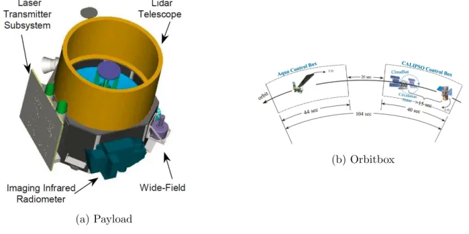
Calipso (Cloud-Aerosol Lidar and Infrared Pathfinder Satellite Observations) is a satellite flown in a sunsynchronos 705km polar orbit with an ascending node equator crossing time of 13:30 local solar time (LST). As part of the A-Train (Afternoon Constellation, see figure 2.3b) Calipso flies in close formation with Aqua, CloudSat, Parasol and Aura. It was launched on 28 April 2006, the orbit tracks repeat every 16 days and its speed is about 7km/s. Its payload consist of CALIOP (Cloud-Aerosol Lidar with Orthogonal Polarization), the IIR (Imaging Infrared Radiometer) and the WFC (Wide Field Camera). These three instruments are near-nadir viewing with an angle of 3.0◦ along track in forward direction since November 2007. Only Caliop is used in this work. Caliop is a diode-pumped Nd:YAG laser which is providing linearly-polarized pulses of light at 1064nm and 532nm with a pulse energy of 110mJ in a pulse rate of 20.2Hz. A 1-m-diameter all-beryllium telescope collects the atmospheric returns of the backscattered intensity at 1064nm and the two orthogonal polarization components at 532nm. The laser beam has a diameter of 70m at the Earth’s surface. The resolution of the lidar is 30m in vertical and 333m in horizontal from surface to 40km of altitude. Further up in the upper troposphere the resolution is 1kmhorizontally and 60mvertically and in the stratosphere 5kmhorizontally and 180m vertically. (Stephens et al., 2002; Winker et al., 1996, 2003, 2007, 2009; Hunt et al., 2009; Mioche et al., 2010)
The main feature used of Caliop in this work is the height of the cloud layer detected by the algorithm called SIBYL (Selective, Iterated Boundary Location). It detects the cloud layers by a dynamic threshold at 532nmfor every shot depending of the ground backscatter and the altitude. It is described detailed by Vaughan et al. (2009)
(a) Payload
(b) Orbitbox
Figure 2.2: Calipso: (a) Payload with Caliop, IIR and WFC (Winker et al., 2003), (b) Orbitbox of CloudSat and Calipso in relation to the Aqua control box (Stephens et al., 2002).
In figure 2.2a you can see an animation of Calipso with its payload (Caliop, IIR and WFC). Figure 2.2b shows the orbit box of Calipso and CloudSat who are following Aqua. Calipso is just 15s (94km) after CloudSat (Platt et al., 2011).
2.2.3
CloudSat
CloudSat is a satellite in the A-train (see figure 2.3b) and flies in the same orbitbox than Calipso (see figure 2.2b). It was launched at the same day as Calipso and follows Aqua with less than 120s. It carries a W band Cloud Profiling Radar (CPR), operating at 94GHz (3.2mm), which is looking near-nadir with an angle of 0.16◦. The antenna has a diameter of 1.85m. The pulse length is 3.3µs. Its vertical resolution is 500mand it delivers measurements from the surface up to about 30km. The field of view (FOV) at the surface is 1.4x3.5km and overlaps with the FOV of Calipso at least 50%. The measurements are averaged in 0.32s time intervals. Due to oversampling the data is presented at 250m vertical resolution (i.e. 125 range bins) and its average time intervals are 0.16s (i.e. every 1.09km on the ground track). The required intensity of clouds to be detected has to be greater than the noise floor of about−29dBZ. (Stephens et al., 2002; Tanelli et al., 2008) In figure 2.3a you can see the layout of CloudSat with insets of photographs of the hardware. Figure 2.3b shows the constellation of the A-Train. First is Aqua, followed by CloudSat and Calipso, then Parasol and finally Aura.
(a) Cloudsat Layout
(b) The A-Train
Figure 2.3: CloudSat: (a) Layout of CloudSat with insets of photographs of actual flight hardware (Stephens et al., 2002), (b) The constellation of the A-Train and its members (Stephens et al., 2002).
The main feature of CloudSat additional to the reflectivity of the CPR used in this work is the cloudmask derived with the aid of MODIS (Moderate-Resolution Imaging Spec-troradiometer) flying on Aqua. The algorithm is described in detail by Ackerman et al. (1998). The algorithm classifies the radar signal in very weak echo, weak echo, good echo and strong echo with the rate of false detection of < 50%, < 16%, < 2%, and < 0.2% respectively.
2.2.4
Meteosat SEVIRI
Meteosat Second Generation (MSG) is the second generation of a geostationary satellite mission. They operate at about 36000km. Aboard of MSG there is the SEVIRI (Spinning Enhanced Visible and InfraRed Imager) instrument. It provides images of the Earth’s full disk with eleven different channels of wavelength every 15 minutes. Its spacial resolution at the sub-satellite point is 3x3km. Additional there is a broadband HRV (High Resolution Visible) channel with a resolution of 1km at the sub-satellite point. The HRV channel covers half of the full disk. For the wavelength of the channels see table 2.1. (Schmetz et al., 2002; Bugliaro et al., 2011, 2012)
Channel λc/µm Spectral interval/µm Sampling distance/km Gas ab-sorption Absorbing gases VIS006 0.64 0.56-0.71 3 Low O3, H2O VIS008 0.81 0.74-0.88 3 Low H2O IR 016 1.64 1.50-1.78 3 Low H2O IR 039 3.90 3.48-4.36 3 Low H2O, CO2, CH4, N2 WV 062 6.25 5.35-7.15 3 High H2O WV 073 7.35 6.85-7.85 3 High H2O IR 087 8.70 8.30-9.10 3 Low H2O IR 097 9.66 9.38-9.94 3 Medium O3 IR 108 10.80 9.80-11.80 3 Low H2O IR 120 12.00 11.00-13.00 3 Low H2O IR 134 13.40 12.40-14.40 3 Medium CO2 HRC 0.75 0.40-1.10 1 Low O3, H2O
Table 2.1: SEVIRI spectral channels with characteristics, central wavelengthλc, spectral interval, sampling distance and gas absorption properties (data from Schmetz et al. (2002); Bugliaro et al. (2012))
In figure 2.4a you can see an animation of the MSG satellite. Figure 2.4b shows the coverage of channels 1-11 of SEVIRI.
(a) Animation of MSG satellite (b) Coverage of SEVIRI
Figure 2.4: Meteosat SEVIRI: (a) Animation of MSG satellite (Schmetz et al., 2002), (b) Coverage of SEVIRI for the channels 1-11 (Schmetz et al., 2002).
Data and Methods
This chapter will be about the data which were used and the methods applied in this work. First the data of the Mira-36 cloud radar, Calipso’s Caliop, CloudSat’s CPR and Meteosat’s SEVIRI are described. Then the methods of the algorithms that were performed are presented.
3.1
Data
In this section there will be explained the used data of Mira-36, Caliop, CPR and SEVIRI. To make the satellite data temporal and geometrical comparable to the fixed point of measurement of the radar, the satellite data have to be selected by choosing a reasonable distance to the radar and in case of Calipso and CloudSat for their speed of about 7km/s.
3.1.1
Mira-36 data
The Mira-36 cloud radar data used in this work are about four years from December 2011 to June 2015. The measurements are stored daily in a NetCDF file. In this file there are the backscatter signal which is corrected by the noise, the Doppler velocity and the linear depolarization ratio saved every ten seconds. Unfortunately there are some gaps in the data because of breakdowns, repairs and maintenances.
3.1.2
Calipso data
The data from Calipso’s Caliop are obtained from the NASA Langley Research Center (LARC) Atmospheric Science Data Center (ASDC). The Level 1B Data in the versions V3-01, V3-02 and V3-30 of the 532nmwavelength are used. They consist of all overpasses of the satellite with a distance of less than 15km around the Mira-36 in the time period of the existing cloud radar files. The data format is the hierarchical data format (HDF). The 15km circle is chosen because this is round about the dimension of the Zugspitze and there are still quite a reasonable amount of overpasses. For smaller radii the amount of
overpasses decreases quick and for larger radii there would be measured clouds over the surrounding mountains.
3.1.3
CloudSat data
The data of CloudSat’s CPR are from the CloudSat Data Processing Center. The Level 2B-GEOPROF in the version R04 are used. They consist of all overpasses of the satellite with a distance of less than 200km around the Mira-36 in the time period of the existing cloud radar files. The data format is HDF. The considered radii in the comparison are 15km, 50km, 100kmand 200km. The radius of 15kmis chosen because of the same reasons of the Calipso data. The bigger radii were chosen to make it comparable to Protat et al. (2009).
3.1.4
Meteosat data
The data of Meteosat SEVIRI contain the Ice Water Path (IWP), the optical thickness and the effective radius of a grid of 15 x 15 pixels around the Schneefernerhaus. Only the pixel where the Mira-36 radar is located and the eight neighboured pixels were used. Bugliaro et al. (2011) derived these parameter with the DLR (German Aerospace Center) APICS (Algorithm for the Physical Investigation of Clouds with SEVIRI) retrieval for June 2014 and for January 2015. The temporal resolution is 5minfor the June 2014 data and 15min for the January 2015 data. The size of the grid cell where the Mira-36 radar is located is about 3.17km x 5.50km. The data format is NetCDF.
3.2
Methods
In this section the methods of the algorithms are explained. First the algorithm of the cloud detection of the Mira-36 cloud radar and the retrieval of the mean diameter and the ice water content are presented. Then the comparison of Calipso with Mira-36, the comparison of CloudSat with Mira-36 and the comparison of SEVIRI and Mira-36 are introduced.
3.2.1
Mira-36 cloud layer detection
For the cloud detection of the Mira-36 an algorithm was developed. It is based on the algorithm of H¨aring (2014). Day by day the needed parameters, time, heights of the range bins, the backscatter signals and the Doppler velocities are imported in the originally ten seconds resolution. First the lowermost ten range bins (that is up to about 300m above the radar) of every timestep of the Doppler velocities are checked for the fall velocity to be smaller than 3m/s. That’s for excluding rain situations. Measurements with rain are marked and further neglected. Then the backscatter signals are tested for the cloud base from bottom to top. If there is an entry, the next three range bins are also checked for a
signal. Only when the cloud is at least three range bins thick (that is about 86,4m) it is stored as the cloud base. This is for excluding single backscatter events like insects, birds or clear sky echoes. For finding the cloud top the backscatter signals are further examined from the previous found cloud base upward. If there are three range bins found with no entry the cloud top is the height of the first range bin and stored. This ensures, that two clouds have to be at least about 86,4m separated and are clearly the next cloud layer. For cloud base and top number two and three the same procedure is applied, starting from the previous top/ base. If there is no cloud detected, no height is saved.
To ensure that the cloud bases/ -tops are longer than 10 s above the radar and to have , depending on the horizontal wind speed, a horizontal dimension, all cloud bases/ tops are checked if at least the temporal previous or ensuring range bin of cloud base/ top not vary more than ±2 range bins (that is about±72m).
The cloud thickness is the difference from the respective cloud top to the cloud base. Finally the range bins are converted to heights above the radar in meters.
3.2.2
Mira-36 mean diameter and IWC
To get the mean diameter of the particlesD0 the one-minute averaged Mira-36 fall velocities
are taken into account. The polynomial fit of the ordern = 1 for gettingD0 out of the fall
velocity Vt found by Matrosov et al. (2002) is applied: D0 = 9.0·10−4Vt3−6.6·10
−2V2
t + 6.2Vt−9.7 (3.1) with Vt ≥0.06m/s.
Out of the mean diameter D0 the Ice Water Content (IWC) is calculated by using the
one-minute averaged Mira-36 reflectivities following Atlas et al. (1995): IW C = Ze
G·D3 0
(3.2) withZethe reflectivity inmm6/m3, IWC ing/m3andD0 inµm. G is a coefficient which is
depending on the bulk density, the shape of the particle and the Particle Size Distribution (PSD) and is like: G= ( 10−6 if D0 ≤50µm 7.5·10−5D−01.1 if D0 >50µm (3.3)
3.2.3
Comparison Calipso - Mira-36
For the comparison of the cloud tops of Calipso and Mira-36 the Calipso data are read in by the day. For all times the distance of the ground track of Calipso to the Schneefernerhaus is calculated after Vincenty (1975). Therefore a WGS84 ellipsoid is supposed with the flattening of f = 1/298.257233563 and with the radius of the Earth of a = 6378.137km (Slater and Malys, 1998). The cloud top of Calipso is the highest cloud top of the inbuilt cloud layer detection SIBYL of Calipso at the nearest distance to the Schneefernerhaus. To
the time of the nearest point of Calipso to the Schneefernerhaus the cloud top of Mira-36 is searched. The time difference is not allowed to be more than 10s because the resolution of the Mira-36 data is ten seconds and so it is the temporal nearest measurement. The backscatter of the radar is now examined from top to bottom and the cloud has to be at least seven range bins thick (about 201.6m) because of the complex threshold and averaging method of SIBYL (Vaughan et al., 2009) the Mira-36 would detect even very small cloud layers which are not detected by SIBYL. This threshold and averaging of SIBYL is also due to the high speed of the Calipso satellite of about 7km/s. Finally the height of the cloud top of the Mira-36 is converted to mean sea level (MSL).
3.2.4
Comparison CloudSat - Mira-36
The following describes algorithm compares the reflectivity, the cloud top height, the cloud thickness, the cloud base height and the mean vertical profile of the radar reflectivity of the Mira-36 cloud radar with the CPR of CloudSat. It is akin to Protat et al. (2009). First the one-minute averaged Mira-36 data (time, reflectivity and range bins) are read in, then the CloudSat data (time, position, range bins, reflectivity and MODIS cloudmask) are read in by the day. The Mira-36 data are now used in a one-minute average because with lager radii around the radar the satellite stays longer is the radius (up to half a minute). Only heights between 3km and 10km above MSL are considered because the radar is already at a height of 2671m above MSL and clouds detected in a valley by CloudSat are not comparable. The distances of CloudSat to the Schneefernerhaus are calculated in the same way as for the Calipso - Mira-36 comparison. Only CloudSat data where the radius around the Mira-36 radar is smaller than a defined radius (15km, 50km, 100km and 200km are used) are kept. In the area of this circle the cloud top and the cloud base are determined. The cloud top is the first range bin, where from top to bottom the value of the MODIS cloudmask is greater than 30 (good echo, <2% false detection (Marchand et al., 2008)) or if the altitude of the echo is higher than 6km, the value of the MODIS cloudmask is greater than 5 (very weak echo, <50% false detection (Marchand et al., 2008)) for detecting high weak cirrus. The cloud base is found in the same way but from bottom to top. After that the mean of the cloud top, the cloud base and the reflectivity profile is calculated. The cloud thickness is the difference of cloud top and cloud base. To get the time of the closest measurement of the Mira-36 to the CloudSat overflight the Mira-36 time is searched for the smallest time difference to the time where the track of CloudSat is perpendicular. At this time the Mira-36 reflectivity is checked for cloud top and cloud base.
3.2.5
Comparison Meteosat SEVIRI - Mira-36
For the comparison of the Ice Water Path (IWP) between SEVIRI and the Mira-36 radar the Ice Water Content (IWC) of the radar is derived in three different ways. The first way is in relation to the reflectivity and the Doppler velocity (IWC-Z-VEL) shown in equation 3.1 and 3.2. But otherwise with a five-minute averaging of the input radar reflectivity and Doppler velocity because of the big influence of the Doppler velocity and because
the Meteosat data is also five-minutes averaged in the June data. The second way is a relation of the reflectivity and the temperature (IWC-Z-T) derived by Protat et al. (2007) for midlatitudes:
log10(IW C) = 0.000372ZdBT + 0.0782ZdB −0.0153T −1.54 (3.4) with ZdB the reflectivity in dB and T the temperature. The used temperature profiles are from the radiosondes launched daily in Innsbruck at 03 UTC. And the third way is a relation of only the reflectivity (IWC-Z) derived by Protat et al. (2007) for midlatitudes:
IW C = 0.082Z0.554 (3.5)
with Z the reflectivity. Then the IWC is integrated over the hight to get the IWP.
For the scatter plots, shown in figure 4.15, the data is compared with a most possibly suitable averaging. The IWC-Z-T and the IWC-Z algorithm are compared to each other with the temporal resolution of the Mira-36 radar (10s) because they are produced by the same device and the same temporal resolution (figure 4.15a). For the comparison between the IWC-Z-VEL and the IWC-Z algorithms (figure 4.15b) the IWC-Z data is averaged
±5min around the nearest data point to the VEL algorithm because the IWC-Z-VEL data are already five-minute averaged because of the updraughts. To compare the IWC-Z algorithm with the one of MSG, the MSG data are averaged with the t0−15min,
t0 and t0 + 15min measurements in January and with the t0 −5min, t0 and t0 + 5min
measurements in June, because in January the time resolution is 15minand in June 5min. The IWC-Z data are averaged at the temporal closest point to the MSG measurement with the ±15min measurements in January and with the ±5min measurements in June. For the scatter plot of figure 4.15d the MSG algorithm is averaged as described before and the IWC-Z-VEL algorithm is averaged similar to the IWC-Z algorithm described before. These averaging methods are akin to the averaging methods applied by Reinhardt et al. (2014).
Results
In this chapter the main results of this work are presented. First the statistical parameters of the Mira-36 cloud radar are investigated, then Mira-36 properties are compared with the according ones of Calipso and CloudSat. And finally Ice Water Path algorithms of Meteosat and Mira-36 are compared.
4.1
Statistical parameters of Mira-36
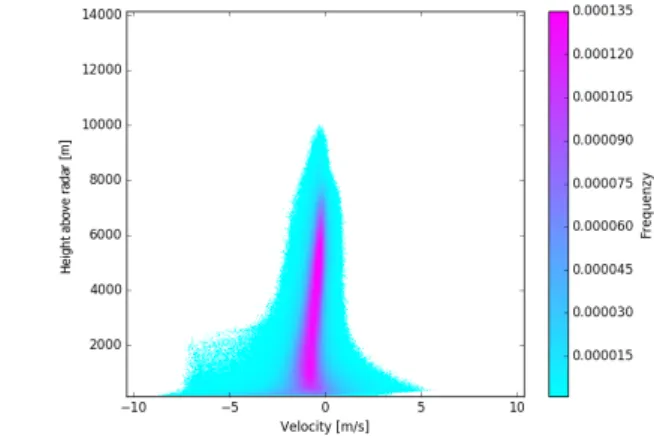
For evaluating the Mira-36 data, the height resolved frequencies of occurrence of all the available data over the reflectivity and the Doppler velocity from December 2011 to June 2015 were represent in figure 4.1. Figure 4.1a shows the height over the reflectivity and figure 4.1b the height over the Doppler velocity. Both have the same appearance as Hagen et al. (2015) did it for the year of 2014.
(a) Joint height-revlectivity histogram (b) Joint height-velocity histogram Figure 4.1: Joint histograms from December 2011 to June 2015, heights are above radar: (a)
Joint height-revlectivity histogram, (b) Joint height-velocity histogram.
above MSL). The reflectivities decreases with the hight from about 10dBZ at radar height to about−40dBZ at altitudes of about 7km above the radar. There is an area of reduced frequencies of about 2 - 4km above the radar. The plume of reflectivities existing between
−10 and 10dBZ at altitudes from the radar up to about 2.0km is caused by precipitation events.
Figure 4.1b shows that the fall velocity increases towards the ground suggested by droplet growth. Because of strong vertical movements over mountains and precipitation the width of the velocity spectrum is broadened. On the lower left side of the diagram the broadening is caused mainly by precipitation, especially snow and some rain.
4.1.1
Cloud fraction
To get more details out of the cloud layer detection algorithm presented in chapter 3 the cloud layer information were further examined and pictured in figure 4.2.
(a) Cloud / no-cloud ratio
(b) Distribution of cloudlayers
Figure 4.2: Cloudfraction above Mira-36: (a) Ratio of cloud and no cloud events, (b) Distribution of the three cloud layers.
Almost half of the time there was no cloud above the Mira-36 radar, illustrated in figure 4.2a. In the other half of the time there were for 62.2% of the time clouds in the height from the radar up to 500m, for 19.9% of the time in the height from 500m up to 3.35km above the radar and for 17.9% of the time heights more than 3.35km over the cloud radar detected. These height classification is introduced in dependence of the standard ´etages of
Kraus (2004) and the cloud base is crucial for the grading. Because of the high altitude the radar is positioned, the low clouds do not exist. They are replaced by a height range from 0 to 500m above the radar and should represent the case when the radar is in the clouds. The next cloud ´etage reaches from 3.2km above MSL to 6.0km above MSL and represents the middle ´etage. Clouds over 6.0km above MSL are classified as high clouds.
4.1.2
Cloud properties
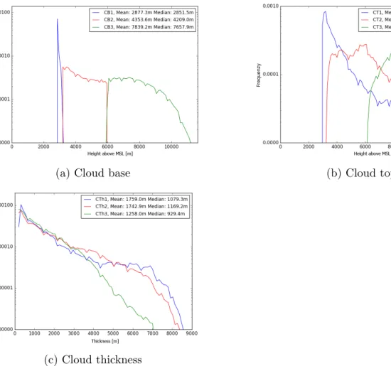
The frequencies over the heights of the previous mentioned cloud classification is repre-sented in figure 4.3. The cloud base is displayed in figure 4.3a, the cloud top in figure 4.3b and the cloud thickness in figure 4.3c. The values of the respective means and the medians are given in the legend of the figures.
(a) Cloud base (b) Cloud top
(c) Cloud thickness
Figure 4.3: Frequencies of the cloud layers in m above MSL: (a) Cloud base, (b) Cloud top, (c) Cloud thickness. In blue is the height range from 2.7km to 3.2km above MSL, in red the height range from 3.2km to 6.0km above MSL and in green above 6.0km.
You can see in figure 4.3a that the most often frequencies of the cloud base are from clouds around the height of the radar and are decreasing with height. The middle ´etage clouds are
almost at the same frequency over the height. The high clouds are decreasing in frequency with height. For the respective cloud tops in figure 4.3b the frequencies of the lower most range is decreasing with height, the frequencies of the middle ´etage is constant up to about 5.5km above MSL and than decreasing with height and the frequencies of the high clouds are first increasing up to a hight of about 9km above MSL and than decreasing. Figure 4.3c represents the cloud thickness. All the cloud thicknesses are decreasing with height almost with the same rate except the high clouds are decreasing faster at a thickness of more than 5km.
4.1.3
Vertical movements
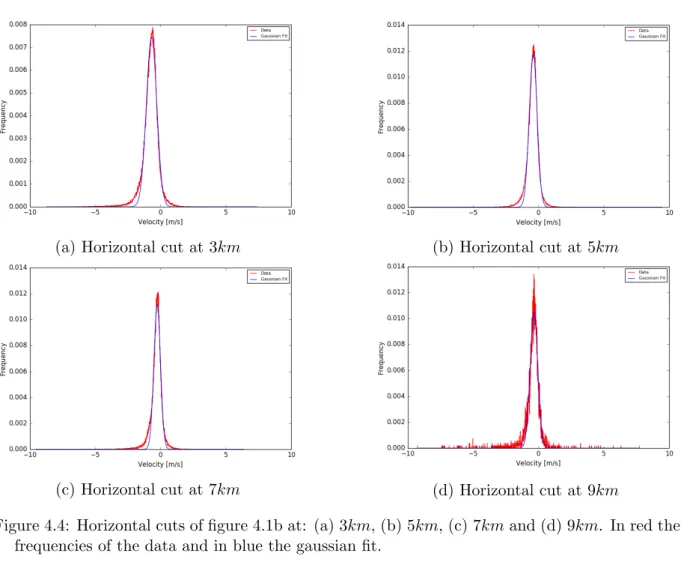
For the further analysis of the vertical motion there were produced four cuts of figure 4.1b. The profiles were represented in figure 4.4. Figure 4.4a, 4.4b, 4.4c and 4.4d represent the four heights of 3, 5, 7 and 9km above the radar respectively.
(a) Horizontal cut at 3km (b) Horizontal cut at 5km
(c) Horizontal cut at 7km (d) Horizontal cut at 9km
Figure 4.4: Horizontal cuts of figure 4.1b at: (a) 3km, (b) 5km, (c) 7kmand (d) 9km. In red the frequencies of the data and in blue the gaussian fit.
In all four figures of figure 4.4 you can see, that the Doppler velocities in red are almost Gaussian shaped and similar to the Gaussian fit in blue. Only at the bottom of the Gaussian
bell there is a broadening with a tendency to greater fall velocities because of precipitation events (here to the negative side). A χ2-distribution-test was performed with a level of significance of 1.0% and all of data in the figures should accept the hypothesis. That means, that to a probability of 99.0% the distributions of the data is Gaussian distributed. In figure 4.4d you can also see, that in the altitude of 9km above the radar (i.e. about 11.7km above MSL) the data is getting rare and the curve gets shaky.
Sometimes there are wave-like phenomena above the Mira-36. For example breaking waves shown in figure 4.5 and 4.6 on 30.09.2012 between 06:57 and 07:48 UTC induced by a wind shear (Hagen et al., 2015). The Doppler velocities of figure 4.5b were further examined. Therefore a horizontal cut is done between 07:12 and 07:40 UTC at 5km altitude above the radar (black solid line in figure 4.5), shown in figure 4.6. A sine fit of the form y=y0+Asin πx−wxcprovides the parametersy0 = −0.22629,A = 2.06225,xc= 15.03587 and w = 17.94911. That makes a frequency of about 10.5h−1 and a mean amplitude of about 2.1m/s.
But otherwise than stationary waves like lee waves these waves observed with the Mira-36 radar at Zugspitze have to be generated somewhere, probably by wind shear, and are somehow advected.
(a) Reflectivity (b) Doppler velocity
Figure 4.5: Breaking wave over Mira-36 at 30.09.2012 between 06:57 and 07:48 UTC: (a) Re-flectivity, (b) Doppler velocitiy. In black is the examined horizontal cut in figure 4.6 at 5km above the radar
Figure 4.6: Horizontal cut of figure 4.5 of the Doppler velocities at 5km above the radar. The measured fall velocities in blue and the fitted sine wave in red.
4.2
Mean diameter and IWC retrievals of Mira-36
To get the mean diameter D0 and the Ice Water Content (IWC) of the Mira-36 the
al-gorithm in chapter 3 is used and the resulting outcome for the 10.11.2012 is illustrated in figure 4.7. Figure 4.7a shows the radar reflectivities, figure 4.7b the Doppler velocities, figure 4.7c the mean diameter and figure 4.7d the Ice Water Content (IWC).
(a) Reflectivity (b) Doppler velocity
(c) Mean diameter (d) IWC
Figure 4.7: Mira-36 retrievals of 10.11.2012 one-minute averaged: (a) The radar reflectivity, (b) The Doppler velocity, (c) The mean diameter and (d) The Ice Water Content (IWC).
Out of the radar reflectivities (figure 4.7a) and the Doppler velocities (figure 4.7b) the mean diameter D0 (figure 4.7c) and the IWC (figure 4.7d) are generated. Only when the
Doppler velocity is negative (i.e. no updraught) the mean diameter is calculated. That results to some gaps in the figure of the diameter. These gaps are still present in the figure of the IWC. Large diameters lead to a small IWC so that their contribution to the IWC is small. But light updraughts that reduce the equilibrium falling speed of the particles lead to a misinterpretation.
4.3
Comparison Calipso with Mira-36
For the comparison of Calipso with Mira-36 the algorithm introduced in chapter 3 is used. The cloud tops of the Mira-36 radar and the Caliop lidar on Calipso are investigated and the results are represented in figure 4.8 and figure 4.9. Figure 4.8 shows the minimal distance of Calipso’s ground track to the 36 and the cloud tops of Caliop and Mira-36 (the dots are connected only for clearness) and figure 4.9 shows a scatter plot of the two identified cloud tops. In the four years of measuring clouds with Mira-36 only 30 overpasses of Calipso within a circle of 15km around the radar are evaluable. Unfortunately there are overpass events where neither the radar did measure well nor Calipso produced usable data. So the data is again reduced down to 17 comparable cloud tops.
Figure 4.8: Cloud tops of Calipso (red) and Mira-36 (green) with the minimum distance of the Calipso ground track to the Mira-36 (blue).
In figure 4.8 you can remark that the the minimum distance of Calipso’s ground track to the Mira-36 is always between 8 and 14km. The passing side of Calipso was allays westerly of Mira-36 (not shown). The laser beam on the Earth’s surface has just a width of 70m, the radar beam is about 130mwide at a distance of 15kmof the radar and the circle of the considered data is 15km around the radar. To compare two devices with a similar narrow
beam and in an area which is large in relation to the beams, is perhaps the reason why the lines in figure 4.8 are looking a bit twitchy. Sometimes the two instruments just see another cloud and therefore get another cloud top. It is also possible, that one of the instruments detects no cloud, where the other one detects a cloud. Also the mountain effects play a role, for example clouds over the ridge or just the fact that next to a mountain normally is a valley where also can be a cloud at altitudes beneath the radar. The different wavelength of the two instruments is recognizable by the detection of very, very small particles. There the lidar is more sensitive. But there are also a few, where the cloud top of both instruments agree within just a few tenth of meters.
Figure 4.9: Scatter plot of cloud tops of Calipso and Mira-36 with the one-on-one line (blue).
Figure 4.9 shows a scatter plot of the cloud tops of Calipso and Mira-36. There it looks much more correlated but due to the few data it is difficult to give a concrete statement. Some points are very close to the one-to-one line, some others are farer away. About half of the data pairs agree within a few hundred meters.
4.4
Comparison CloudSat with Mira-36
For the comparison from the Cloud Profiling Radar (CPR) of CloudSat, acting at 94GHz, to Mira-36, acting at 35.2GHz, the algorithm presented in chapter 3 is used. The frequen-cies of occurrence over the reflectivities, the cloud tops, the cloud thicknesses and the cloud base as the height over the mean of the reflectivities are analysed. Therefore the data of the CPR are considered in a circle around the Mira-36 of 15km(figure 4.10), 50km (figure 4.11), 100km (figure 4.12) and 200km (figure 4.13). Similar to the comparison of Calipso with Mira-36 there are just a few comparable data with the small circle of 15km that’s why the radius is increased stepwise up to the circle of 200km. The considered heights are between 3 and 10km above MSL. The measurements below 3km are neglected.
Figure 4.10: Statistical comparison of CloudSat (red) and Mira-36 (green) with a maximum distance of 15km. The upper left picture shows the radar reflectivity spectra with dashed lines the mean of the respective spectra and the number the difference of these means, the upper one in the middle the heights of the cloud tops, the left one on the bottom the cloud thicknesses, the middle one on the bottom the heights of the cloud bases and the one on the right the mean vertical profiles of the radar reflectivities
In figure 4.10 you can see a very good agreement of the reflectivities. The means of both instruments differ only by 0.8dBz. The cloud top, cloud thickness and cloud base dither
due to the few evaluable overpasses (only 19). But it is much better than at the Calipso -Mira-36 comparison. This is due to the bigger Field Of View (FOV) of CloudSat. The FOV of CloudSat is 1.4 x 3.5kmand this is much more in the dimension of the 15kmcircle than the narrow Caliop beam. At the height profile of the reflectivities you can see, that the reflectivity of CloudSat is less between 3 and 3.5kmbecause of the bigger attenuation of a 95GHz radar and CloudSat is measuring from top to bottom, while Mira-36 is measuring from bottom to top. Also Mira-36 seems to detect more lower cloud bases than CloudSat.
Figure 4.11: Like figure 4.10 with a maximum distance of 50km.
Figure 4.11 shows the measurement with a circle of 50km around the Mira-36 radar. The means of the reflectivities differ a little bit more (2.3dBz) but still agree well. The dithering of the cloud tops, cloud thicknesses and cloud bases are still hight (30 evaluable overpasses). In the range between 3 and 3.5kmabove MSL the difference of the mean reflectivity profile of CloudSat to the Mira-36 one is smaller than at the 15kmrange. But now the CloudSat profile is below the Mira-36 profile in the range up to 5.5km above MSL.
In figure 4.12 the circle around Mira-36 has continued to increased to 100km. The amount of evaluable overpasses increases to 53. The difference of the mean reflectivities increases just a little to 2.5dBz and still agrees well. Now the dithering of the cloud tops, cloud