Incremental Specification and Analysis
in the Context of Coloured Petri Nets
by Glenn Anthony Lewis
I hereby declare that this thesis contains no material which has been accepted for a de-gree or diploma by the University of Tasmania or any other institution, except by way of background information duly acknowledged in the thesis, and to the best of my knowledge and belief no material has been previously published or written by another person except where due acknowledgement is made in the text of the thesis.
This thesis may be made available for loan and limited copying in accordance with the Copyright Act 1968.
Glenn Lewis, January 11, 2002
The great thing is to last and get your work done and see and hear and learn and understand; and write when there is something that you know ...
ERNEST HEMINGWAY - DEATH IN THE AFTERNOON
Acknowledgements
In an interview for a Ph.D. scholarship I was asked what I thought I would need to suc-cessfully complete a Ph.D. My answer focused on the financial and hardware assistance I would need. Indeed such assistance is essential, but as my interviewers pointed out, even more important than financial assistance is support from mentors, family and friends. This thesis would not have been completed without this support.
First and foremost I thank my supervisor Dr Charles Lakos. Charles has guided me throughout my candidature and assisted me greatly in all aspects of my Ph.D. The work presented in this thesis extends earlier work by Charles on Coloured Petri Net refinements and many of the ideas presented in this thesis have resulted from discussion with Charles. The fact that there has been a distance of at least 1000Icm between our homes for all but the first six months of my candidature has meant that much of this discussion has been by email. That this form of communication has been effective is a testament to Charles' commitment and effort.
When Charles decided to take up a senior lecturing position at the University of Ade-laide, Dr Vishv Malhotra agreed to act as my official supervisor at the University of Tas-mania. I thank Vishv for this, and for his comments and advice throughout the course of my research.
The algorithms presented in Chapter 7 were implemented in an existing reachability tool. I thank Thomas Mailund and Soren Christensen for their comments on the suitability of the Design/CPN tool, Peter Starke for his comments on the suitability of the INA tool, and Marko Makela for his comments on the suitability of the Maria tool. The Maria tool of the Theoretical Computer Science Laboratory, University of Helsinki, was the tool chosen, and much of the implementation of the algorithms was achieved during an eight month visit to the Laboratory. I thank Nisse Husberg and the other members of the Laboratory for their assistance during this time.
The algorithms were tested on some case studies, including the Missile Simulator study of Steven Gordon and Jonathan Billington. I thank Steven Gordon for supplying a copy of his implementation of the Missile Simulator for comparison with my own im-plementation.
I am grateful to Nicole Clark and Scott Rayner for proofreading, and Julian Dermoudy for surrendering his computer to me while he was on leave. I also thank the anonymous examiners for their comments helping to improve the quality of the thesis. Finally, I thank my parents for their support and encouragement throughout my entire education, and I thank my friends — Fiona, Bob, Scotty, Disco, Mat, Munna, Stu-D, and everyone from Tae Kwon Do — for their support and for the distractions.
This work has been funded by an Australian Postgraduate Award Scholarship, ARC Large Grant A49800926, and University of Tasmania Department of Computing Top-up Scholarship.
Glenn Lewis, Hobart, January 11, 2002
Abstract
Incremental development involves creating a new specification or implementation by mod-ifying an existing one. This is a commonly used technique for handling complex systems in hardware and software engineering. In fact, incremental development is fundamental to object-orientation, the widely adopted approach to software engineering which uses the mechanism of inheritance.
Incremental development and object-orientation have been adopted for all phases of software engineering, from analysis to design and implementation. In the domain of con-current systems, some researchers constrain incremental development by proposing re-quirements that must hold between the original and incrementally modified components. Such proposals are commonly based on a process algebra correctness relation, or require that a bisimulation relation hold between the original and modified components.
In Part I of this thesis we provide background on constraining incremental change and survey several existing proposals. We identify a number of problems typical of these pro-posals which commonly limit their practical use. We then present Incremental Coloured Petri Net Modelling which is aimed at addressing these problems. The main contribution of this part of the thesis is the identification of these problems and the assessment of the practical applicability of Incremental Coloured Petri Net Modelling. This assessment is made by examining several case studies published in the literature.
One of the primary benefits of using a formal method such as Coloured Petri Nets (CPNs) is its support for formal reasoning. State space analysis is a popular formal rea-soning technique, but it is subject to state space explosion, where its application to real world models leads to unmanageably large state spaces.
In Part II of this thesis we first review existing approaches for alleviating the state space explosion problem. The main contribution of Part II is a new approach, which we call Incremental Analysis. Incremental Analysis involves algorithms which take advan-tage of Incremental CPN Modelling in attempting to alleviate the state space explosion problem. The thesis considers the implementation issues for these algorithms, identifies the situations under which they can be expected to lead to performance improvement, and presents case studies which demonstrate the value of the technique.
Contents
1 Introduction 1
1.1 Motivation 1
1.1.1 Embedded Systems 2
1.1.2 Critical Systems 3
1.1.3 Protocol Development and Analysis 3
1.2 Problem Statement 3
1.3 Contribution of the Thesis 4
1.4 Overview 4
2 Background 5
2.1 Object-Orientation 5
2.2 Formalisms for Concurrent Systems 8
2.2.1 Low-Level Net Systems 9
2.2.2 High-Level Petri Nets 11
2.2.3 Modular Petri Nets 17
2.2.4 Object-Oriented Petri Nets 17
2.3 Behavioural Compatibility for Concurrent Systems 18
2.4 Summary 20
I Incremental Specification 22
3 Existing Approaches to Incremental Change 23
3.1 Appropriate Incremental Development 23
3.2 Constraining Incremental Development 25 3.2.1 Proposals for Behavioural Subtyping 27 3.2.2 Constraints on Incremental Change in Practice 30
3.3 Summary 32
4 Incremental CPN Modelling 33
4.1 A Simple Example 33
4.2 Formalising Refinements 38
4.3 CPN Morphisms 39
4.4 Type Refinement 42
4.5 Subnet Refinement or Extension 43
4.6 Node Refinement 44
4.7 Relationship with Equivalences (cf Section 2.3, fig 2.7) 47
4.8 Summary 51
5 Incremental CPN Modelling In Practice 53
5.1 Checking Incremental Change 54
5.2 Case Studies 54
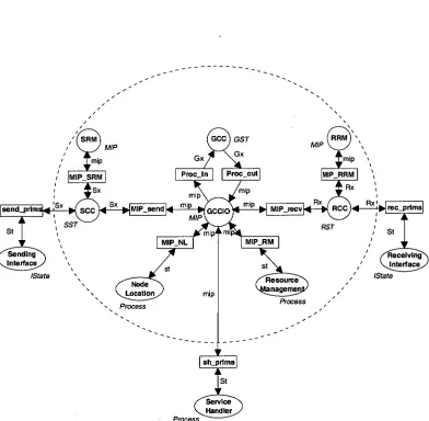
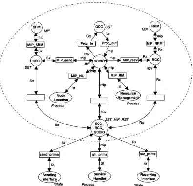
5.2.1 Designing and Verifying a Communications Gateway Using CPNs 55
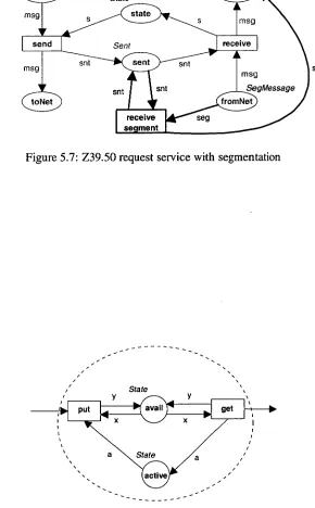
5.2.2 The Z39.50 Protocol 59
5.2.3 Fieldbus Protocol 63
5.2.4 Modelling a Die Bonder with Object-Oriented Timed Petri Nets 64
5.2.5 Air-to-Air Missile Simulator 66
5.2.6 Case Study Summary 69
5.3 Incremental CPN Modelling Applied to the UML 69
5.4 Summary 71
II
6
Incremental Analysis
State Space Reduction Methods
6.1 Formal Reasoning Techniques 6.2 State Space Reduction Strategies
6.2.1 Removing Information 6.2.2 Compression
6.2.3 Compositional Techniques 6.2.4 Preprocessing
6.2.5 Partial State Space Exploration
6.3 Survey of Efficient State Space Reduction Techniques 6.3.1 Partial Order Reduction
6.3.2 Equivalence Reduction
76 76
72
73
73 75 75 76
6.3.3 Binary Decision Diagrams 81
6.3.4 Holzmann's Bitstate Hashing 81
6.3.5 Modular State Spaces 82
6.3.6 Parameterised Reachability Analysis 84
6.3.7 Abstraction 84
6.3.8 Reduction Theory 84
6.3.9 Combining Methods 85
6.3.10 Summary 86
7 Incremental State Space Algorithms 88
7.1 The Standard State Space Algorithm 89
7.2 Catering for Type Refinement 92
7.3 Catering for Subnet Refinement 93
7.4 Catering for Node refinement 96
7.4.1 Informal Explanation of the RNSS 96 7.4.2 Introduction to the Formal Definitions of the RNSS 100
7.4.3 Strongly Connected Components 102
7.4.4 Global Vertices 102
7.4.5 Global Successors 104
7.4.6 RNSS Definition 107
7.4.7 Unfolding the RNSS 108
7.4.8 The RNSS Algorithm 115
7.4.9 Properties of the RNSS 119
7.4.10 Reachability 122
7.4.11 Dead Markings 123
7.4.12 Home Properties 125
7.4.13 Liveness 127
7.4.14 Boundedness 130
7.4.15 An Optimisation to the RNSS Algorithm 131 7.4.16 Comparison to Modular Analysis 140
7.5 Incremental Algorithm 144
7.5.1 Combining the Type and Subnet Algorithms 144 7.5.2 Combining the Type, Subnet, and Node Algorithms 145
8 Implementing the Incremental Algorithms 149
8.1 The Maria Analyser 150
8.1.1 The Front-end Parser Module 151
8.1.2 The Internal Representation 152
8.1.3 The State Module 153
8.1.4 The Transition Analysis Module 155
8.1.5 The Method Module 155
8.1.6 The User Interface Module 155
8.2 Modifications to the Front-end Parser Module 156 8.2.1 Detecting Type and Subnet Refinement 156
8.2.2 Describing Supemodes 158
8.3 Modifications to the Internal Representation 160 8.3.1 The Internal Representation of Superplaces 161 8.3.2 The Internal Representation of Supertransitions 161
8.3.3 Lists of Global Markings 162
8.4 Modifications to the State Module 163 8.4.1 Replacing the Marking of a Place 163 8.4.2 Creating Multiple Reachability Graphs 164 8.4.3 Modifications to the Encoding and Decoding Algorithms 165 8.4.4 Storing Strongly Connected Components 166 8.5 Modifications to the Method Module 166 8.5.1 Finding Enabled Refined Firing Elements 167 8.5.2 Implementing the UPDATE Function 168 8.5.3 Implementing the CHANGED and MAPPED Functions 169 8.5.4 Implementing the ABSTRACTEDGESFROM Function 169 8.5.5 Implementing the comPuTESCCs Function 171 8.6 Modifications to the Transition Analysis Module 171 8.7 Modifications to the User Interface Module 171
8.8 Summary 172
9 Performance of the Incremental Algorithms 173
9.1 Cost of Computing SCCs 174
9.2 Net Properties Affecting Performance 176 9.2.1 Time Taken to Construct the Abstract Graph 178 9.2.2 Number of Disabled Firing Elements 179
9.2.3 Calculating Successors 180
9.2.4 Memory Usage 181
9.2.5 Number of Changed Transitions 182
9.2.6 The Amount of Data Stored in the Tokens 186 9.2.7 Number of Places and Transitions Added by Subnet Refinement 187
9.2.8 RNSS Algorithm 188
9.2.9 Summary 194
9.3 Z39.50 Protocol 195
9.3.1 Implementing the Basic Z39.50 Model 195
9.3.2 Performance with Segmentation 196
9.3.3 Performance with Access Control 198 9.3.4 Performance with Segmentation and Access Control 199
9.4 Air-to-Air Missile Simulator 200
9.5 Summary 208
10 Conclusions and Future Work 209
10.1 Contribution of the Thesis 209
10.1.1 Part I — Incremental Development 209 10.1.2 Part H — Incremental Analysis 211
10.2 Future Work 213
A The Unified Modelling Language (UML) 215
A.1 Class Diagrams 215
A.2 Statechart Diagrams 216
B Tarjan's Algorithm to compute SCCs 218
C Results 220
D Publications 235
D.1 Conference Papers 235
D.2 Workshop Papers and Reports 236
References 238
List of Figures
2.1 The object-based paradigm refined to the object-oriented paradigm (mod-
ified from [199, P. 1691) 7
2.2 Varieties of Polymorphism [43, p. 476] 7
2.3 A net with one token in place pi 10
2.4 The net of Figure 2.3 after transition ti fires 10 2.5 Dining Philosophers Elementary Net System 11 2.6 Dining Philosophers Coloured Petri Net 12 2.7 The linear-time/branching hierarchy [195, p. 280] 19
3.1 The three relationships distinguished [126, p. 58] 25 3.2 A valid incremental change according to van der Aalst and Basten 28 3.3 ATM example (modified from [202, p. 8]) 29
4.1 Crate sending example [3, p. 34] 34
4.2 The crate sending model refined using subnet refinement [3, p. 35] . 35 4.3 Canonical place refinement [116, p. 326] 36 4.4 Subnet indicating the transit of crates 37 4.5 Canonical transition refinement [116, p. 328] 37
4.6 Refined processCrate transition 38
5.1 Abstract model of a communications gateway 56 5.2 Refinement of the communications gateway 57 5.3 Equivalent refinement of the communications gateway 58
5.4 Z39.50 request service 59
5.10 An abstract model of a Die Bonder 65 5.11 The first refinement of the Die Bonder 65 5.12 The second refinement of the Die Bonder 66 5.13 Abstract model of a missile simulator 67 5.14 Refined model of a missile simulator 68 6.1 Dining philosophers reachability graph 74 6.2 A simple CPN (a) and its reachability graph (b) for illustrating the sleep
set method 79
6.3 A BDD for (vi A v2) V (v3 A v4) [194, p. 4961 81
6.4 A modular Place/Transition net [51, p. 228] 83 6.5 The modular state space of the net of Figure 6.4 [51, p. 229] 83
6.6 Simplification of an implicit place 85
6.7 Post-fusion of transitions 85
7.1 A simple net (a) and its reachability graph (b) 89 7.2 The net of Figure 7.1 refined using subnet refinement 94 7.3 The net of Figure 7.1 refined using node refinement 97 7.4 RNSS generation for the net of Figure 7.3 98 7.5 finish transition added to the canonical basis of a supertransition 131 7.6 Semaphore place added to the canonical basis of a supertransition . . . 140 7.7 Two modules both with finite graphs, but the full reachability graph is
infinite [51, p.229] 141
7.8 The net of Figure 7.7 transformed to use transition fusion [51, p.229] . 141
7.9 A modular CPN 143
7.10 The modular state space of the net of Figure 7.9 143 8.1 The modular structure of the Maria analyser (modified from [96, p. 5]) . 150 8.2 A simple net and its Maria net description 152 8.3 The classes Maria uses to represent a net 153 8.4 The classes Maria uses to store the state space 153 8.5 A type and subnet refinement of the net of Figure 8.2 and the Maria
im-plementation 157
8.6 A net with a superplace and the Maria net description 159 8.7 A net with a supertransition and the Maria net description 159 8.8 The modified class diagram of the classes Maria uses to represent a net. 160
8.9 Jensen's Database Manager 165
8.10 Disk space overhead of storing place offsets for each marking of the Database
Managers Net 165
8.11 Time overhead of storing place offsets for each marking of the Database
Managers Net 166
9.1 A net where it is beneficial to compute SCCs 174 9.2 Time improvement when computing SCCs for the net of Figure 9.1 . . . 175 9.3 Space improvement of computing SCCs for the net of Figure 9.1 175 9.4 Time for computing SCCs for the net of Figure 9.1 (without tn+1) 176 9.5 Space overhead for computing SCCs for the net of Figure 9.1 (without
In+1) 176
9.6 An abstract net (a) and a refinement of it (b) 177 9.7 The performance of the type-subnet algorithm on the nets of Figure 9.6 as
the number of states of the refined graph increases 178 9.8 The performance of the type-subnet algorithm on the nets of Figure 9.6 as
the number of disabled firing elements is increased 179
9.9 Modified output arc function 180
9.10 The performance of the type-subnet algorithm on the nets of Figure 9.6 as the complexity of the arc functions is increased 181 9.11 The performance of the type-subnet algorithm on the nets of Figure 9.6 as
the amount of available RAM is increased 182 9.12 The performance of the type-subnet algorithm on the nets of Figure 9.6 as
the number of refined places in the net of Figure 9.6 (b) is increased 183
9.13 One refinement of Figure 9.6 (a) 185
9.14 Another refinement of Figure 9.6 (a) 185 9.15 The performance of the type-subnet algorithm on the nets of Figure 9.6 as
the amount of data in non-refined tokens is increased 186 9.16 The performance of the type-subnet algorithm on the nets of Figure 9.6 as
the amount of data in refined tokens is increased 187 9.17 The net of Figure 9.6 (a) refined by subnet refinement 188 9.18 The performance of the type-subnet algorithm on the nets of Figure 9.6 (a)
and Figure 9.17 as transitions are added to the net of Figure 9.17 188
9.19 A net with a superplace 189
9.20 A net with a supertransition 190
9.21 The time performance of the RNSS for the superplace example (Figure 9.19) 191 9.22 The time performance of the RNSS for the supertransition example (Fig-
ure 9.20) 192
9.23 The disk space performance of the RNSS for the superplace example (Fig-
- ure 9.19) 192
9.24 The disk space performance of the RNSS for the supertransition example
(Figure 9.20) 192
9.25 The time performance of the RNSS for a net with several copies of the
superplace of Figure 9.19 193
9.26 The disk space used by the RNSS for a net with several copies of the
superplace of Figure 9.19 193
9.27 The time performance of the RNSS for a net with several copies of the
supertransition of Figure 9.20 193
9.28 The disk space used by the RNSS for a net with several copies of the
supertransition of Figure 9.20 194
9.29 Z39.50 client 196
9.30 Z39.50 server 197
9.31 Performance of the algorithms for the Z39.50 protocol refined to include
access control 199
9.32 The time for the (standard) RNSS algorithm and standard algorithm as the initial distance between the target and missile is increased for the net of
Figure 5.14 202 9.33 The disk space used by the full reachability graph and the (standard) RNSS
as the initial distance between the target and missile is increased for the net
of Figure 5.14 202 9.34 Refined missile simulator model with canonical Outputs superplace . . 203 9.35 The time for the (standard) RNSS and standard algorithms as the initial
distance between the target and missile is increased for the net of
Fig-ure 9.34 204 9.36 The disk space used by the full reachability graph and the (standard) RNSS
as the initial distance between the target and missile is increased for the net
of Figure 9.34 204
9.37 Refined missile simulator model 206
9.38 The time for the RNSS and standard algorithms as the initial distance be-tween the target and missile is increased for the net of Figure 9.37 . . . . 207 9.39 The disk space used by the full reachability graph and RNSS as the initial
distance between the target and missile is increased for the net of Fig-
ure 9.37 207
A.1 A class diagram represented using the UML 215 A.2 A UML state machine of a home thermostat [33, fig. 21-1] 217
A.3 A complex state [171, fig. 13-55] 217
List of Tables
5.1 Summary of case studies 69
6.1 Summary of efficient state space techniques 87
C.1 Disk space overhead of storing place offsets for each marking of the Database Managers Net (graphed in Figure 8.10) 220 C.2 Time overhead of storing place offsets for each marking of the Database
Managers Net (graphed in Figure 8.11) 220 C.3 Time improvement when computing SCCs for the net of Figure 9.1 (graphed
in Figure 9.2) 221
C.4 Space improvement of computing SCCs for the net of Figure 9.1 (graphed
in Figure 9.3) 221
C.5 Time for computing SCCs for the net of Table 9.1 (without tn+1) (graphed
in Figure 9.4) 221
C.6 Space overhead for computing SCCs for the net of Table 9.1 (without tn+i)
(graphed in Figure 9.5) 222
C.7 The performance of the type-subnet algorithm on the nets of Figure 9.6 as the number of states of the refined graph increases (graphed in Figure 9.7) 222 C.8 The performance of the type-subnet algorithm on the nets of Figure 9.6 as
the number of disabled firing elements is increased (graphed in Figure 9.8) 223 C.9 The performance of the type-subnet algorithm on the nets of Figure 9.6 as
the complexity of the arc functions is increased (graphed in Figure 9.10) . 223 C.10 The performance of the type-subnet algorithm on the nets of Figure 9.6 as
the amount of available RAM is increased (graphed in Figure 9.11) . . . . 224 C.11 The performance of the type-subnet algorithm on the nets of Figure 9.6
as the number of refined places in the net of Figure 9.6 (b) is increased (graphed in Figure 9.12) 224 C.12 The performance of the type-subnet algorithm on the nets of Figure 9.6
as the amount of data in non-refined tokens is increased (graphed in Fig-
ure 9.15) 225
C.13 The performance of the type-subnet algorithm on the nets of Figure 9.6 as the amount of data in refined tokens is increased (graphed in Figure 9.16) 225
C.14 The performance of the type-subnet algorithm on the nets of Figure 9.6 (a) and Figure 9.17 as transitions are added to the net of Figure 9.17 (graphed
in Figure 9.18) 226 C.15 The time performance of the RNSS for the superplace example (Figure 9.19)
(graphed in Figure 9.21) 226
C.16 The time performance of the RNSS for the supertransition example (Fig-
ure 9.20) (graphed in Figure C.16) 227
C.17 The disk space performance of the RNSS for the superplace example (Fig-
ure 9.19) (graphed in Figure 9.23) 227
C.18 The disk space performance of the RNSS for the supertransition example (Figure 9.20) (graphed in Figure 9.24) 228 C.19 The time performance of the RNSS for a net with several copies of the
superplace of Figure 9.19 (graphed in Figure 9.25) 229 C.20 The disk space used by the RNSS for a net with several copies of the
superplace of Figure 9.19 (graphed in Figure 9.26) 229 C.21 The time performance of the RNSS for a net with several copies of the
supertransition of Figure 9.20 (graphed in Figure 9.27) 230 C.22 The disk space used by the RNSS for a net with several copies of the
supertransition of Figure 9.20 (graphed in Figure 9.28) 231 C.23 Performance of the algorithms for the Z39.50 protocol refined to include
access control (graphed in Figure 9.31) 231 C.24 The time for the (standard) RNSS algorithm and standard algorithm as the
initial distance between the target and missile is increased for the net of Figure 5.14 (graphed in Figure 9.32) 232 C.25 The disk space used by the full reachability graph and the (standard) RNSS
as the initial distance between the target and missile is increased for the net of Figure 5.14 (graphed in Figure 9.33) 232 C.26 The time for the (standard) RNSS and standard algorithms as the initial
distance between the target and missile is increased for the net of Fig-ure 9.34 (graphed in FigFig-ure 9.35) 233 C.27 The disk space used by the full reachability graph and the (standard) RNSS
as the initial distance between the target and missile is increased for the net of Figure 9.34 (graphed in Figure 9.36) 233 C.28 The time for the RNSS and standard algorithms as the initial distance
be-tween the target and missile is increased for the net of Figure 9.37 (graphed
in Figure 9.38) 234 C.29 The disk space used by the full reachability graph and RNSS as the initial
distance between the target and missile is increased for the net of Fig-ure 9.37 (graphed in FigFig-ure 9.39) 234
List of Acronyms
Following is a list of the acronyms that are used in this thesis.
ALU = Arithmetic (and) Logic Unit ATM = Automatic Teller Machine BDD = Binary Decision Diagram CCA = Call Control Application
CCS = Calculus of Communicating Systems CLOWN = CLass Orientation With Nets
COOPL = Concurrent Object Oriented Programming Language
CO-OPN = Concurrent Object Oriented Petri Nets CORBA = Common Object Request Broker Architecture
CPN = Coloured Petri Net
CSP = Communicating Sequential Processes CTL = Computation Tree Logic
DDD = Data Display Debugger DLE = Data Link Element DLL = Data Link Layer
DPE = Distributed Processing Environment EN-system = Elementary Net System
GNU = GNU's Not Unix GUI = Graphical User Interface HCPN = Hierarchical Coloured Petri Net
HEC = Hydro-Electric Corporation (of Tasmania) HLPN = High Level Petri Net
HTTD = Hierarchical Timed Transition Diagram
ISA = International Society for Measurement and Control ISDN = Integrated Services Digital Network
LAS = Link Access Scheduler LEN = Labelled Elementary Net
LOOPN = Language for Object Oriented Petri Nets LOTOS = Language Of Temporal Ordering Specification
LTL = Linear Temporal Logic LTS = Labelled Transition System ODP = Open Distributed Processing
OLST = Observable Local State Transformation 00 = Object-Oriented
00PL = Object-Oriented Programming Language 00PN = Object-Oriented Petri Net
00SE = Object-Oriented Software Engineering OPN = Object Petri Net
PN = Petri Net
PTN = Place Transition Net RAM = Random Access Memory
RCC = Receiving Call Control RG = Reachability Graph
RS = Request Substitutability RNSS = Refined Node State Space
SCC = Strongly Connected Component
SDL = Specification and Description Language SRM = Sending Resource Management
SSM = State Space Method ST = State Transformation STD = State Transition Diagram SSM = State Space Method
TINA = Telecommunications Informations Networking Architecture UML = Unified Modelling Language
Chapter
1
Introduction
1.1 Motivation
Concurrent systems are systems composed of elements that can operate concurrently and communicate with each other [79]. The majority of large systems are concurrent [167], and as Meyer says "Concurrency is quickly becoming a required component of just about every type of application, including some which had traditionally been thought of as fun-damentally sequential in nature" [140, p. 951].
Concurrent software systems are inherently more complex than sequential software systems. This complexity arises because concurrent systems:
• introduce non-determinism; that is, given the same input and initial state the system can produce several different output states.
• usually exhibit an extremely large number of different behaviours due to the large number of possible interactions between components of the system.
• have design concerns that are not apparent in sequential systems such as locality and synchronisation.
The complexity of concurrent software systems means they are notably difficult to design [205, 140, 79]. To combat the complexity of a concurrent system it is widely recommended that aformal model of the system be developed [139, 18, 34, 87, 92, 144]. A formal model is a mathematically based description of the system that allows for reasoning about system properties.
Many formal modelling techniques have been proposed, including process algebras [141, 142, 91, 90, 24, 98], and Petri Nets [158, 102, 164, 78, 3]. Petri Nets are seen to have many positive attributes including: their graphical representation; their even-handed treatment of state and change of state; their ability to be simulated; their well-defined semantics; their ability to be used to represent systems at different levels of abstraction; and their ability to model true concurrency rather than interleaving semantics [145, 185, 102, 162]
Usually the development of a formal model is an incremental process that begins with an abstract model. The abstract model is then refined, possibly over several iterations, to a more concrete model. In fact incremental development is fundamental to object-orientation (see Chapter 2), one of the most widely used software engineering methods. In
CHAPTER 1. INTRODUCTION 2 object-orientation, incremental development is achieved through inheritance, where a new specification or implementation is developed by inheriting and incrementally changing an existing specification or implementation. Several proposals have been made to integrate Petri Nets and object-orientation [113, 22, 28, 71, 177].
The integration of object orientation and formal methods has seen a focus on the rela-tionship between the original and incrementally changed component. This has lead some researchers to propose compatibility rules between the original and incrementally changed component [116, 60, 169, 148, 35, 17, 7, 17].
One of the main benefits of developing a formal model is that the model can be for-mally analysed. Here we use the term formal analysis in a broad sense to mean answering formal questions about a system's behaviour. Formal analysis therefore encompasses ver-ification (mathematically proving if a formal system has a formally stated property), error detection (finding errors in a system), as well as general questions such as "What is the maximum number of messages simultaneously in this queue?".
We note that testing (unless it is exhaustive) cannot be used to verify the correctness system [68]. In order to verify (i.e mathematically prove) that a system conforms to a property, all possible behaviours of the system have to be checked.
State based methods are one of the most successful strategies for the formal analysis of concurrent systems. They commonly involve exploring a global state graph representing all behaviours of the system. A major advantage of state based methods is that they are generally automatic and do not require highly skilled personnel.
Formal modelling and analysis is seen as essential in many domains, including embed-ded systems, safety and security critical systems, and protocol development and analysis. In the following sections we consider these domains in more detail, particularly their need for formal modelling and analysis.
1.1.1 Embedded Systems
An embedded system is one that is physically embedded within a larger system, the pri-mary purpose of which is to maintain some property or relationship between other com-ponents of the system [161]. Embedded systems are everywhere, they appear in just about anything electronic including cars, consumer electronics and computer peripherals. It is expected that the number of embedded systems will continue to grow rapidly due to the continued decrease in size and cost of microprocessors, and an increased desire to network systems that have not traditionally been networked.
Embedded systems are often even more complex than non-embedded systems because they must frequently encompass one or more of the following characteristics:
• real-time (the output of the system is dependent on the input and time). • reactive (the system is in continual interaction with its environment)
CHAPTER 1. INTRODUCTION 3
1.1.2 Critical Systems
By their very definition, safety-critical systems such as aircraft controllers (e.g. Rushby [172]), medical systems (e.g. Ladeau [111]), and nuclear power plant controllers (e.g. Archinoff [14]) must satisfy certain requirements. Formal analysis provides the opportu-nity to significantly increase confidence that these requirements are satisfied in the final system. For this reason, the use of formal methods has been strongly advocated for such systems [34, 85, 18].
With the explosive growth of the World Wide Web, there is increasing consumer de-mand for secure access to electronic commerce systems such as money transfer, stock market and electronic shopping. Errors in such security-critical systems are simply not acceptable. To verify the correctness of security-critical components, we must be able to answer the question: is a particular state reachable from the initial state? [157] Formal analysis is the only practical way to answer such questions.
1.1.3 Protocol Development and Analysis
The development of new technologies such as satellite communication, intelligent man-ufacturing systems, global education products, transport systems and multimedia appli-cations (voice, data, images, video), all rely on various protocols. The consequences of failure of such protocols cannot be overstated; millions of dollars, and/or loss of life could be expected. As Needham et al [146, p. 999] say, protocols are prone to subtle errors that are" ... unlikely to be detected in normal operations. The need for techniques to verify the correctness of such protocols is great ... ". As an example of this, in a paper published in 1996, Lowe [134] breaks the Needham-Schroeder public-key protocol first proposed in 1978. It is often vitally important that protocols are verified to work correctly under all situations. This is something that can only be done using formal modelling and analysis.
1.2 Problem Statement
This thesis addresses two main problems:
Problem I: In the domain of formal modelling for concurrent systems many of the proposals constraining incremental change are aimed at guaranteeing that the incre-mentally changed component can be substituted for the original component, without the environment being able to detect the difference. Concerns have been raised that such constraints for substitutability are too strong for use in practice [201]. It is not clear what is required for use in practice, and whether a recent proposal by Lakos [116] is appropriate.
CHAPTER 1. INTRODUCTION 4
1.3 Contribution of the Thesis
The first part of this thesis examines existing approaches to constraining incremental de-velopment and identifies problems with the applicability of such approaches in practice. The approach developed by Lakos [116] — Incremental CPN Modelling — is presented and its practical applicability examined. The main contribution of this part of the thesis is the identification of problems typical of existing proposals and the assessment of the practical applicability of Incremental CPN Modelling.
In the second part of this thesis we present algorithms that help alleviate the state space explosion. These algorithms take advantage of each of the forms of incremental change introduced in the first part of the thesis and are referred to as incremental algorithms. We discuss the implementation of the incremental algorithms and examine the conditions under which they can be expected to lead to performance improvements. We also examine the performance of the algorithms for some case studies.
It is also worth noting what this thesis does not address. Although this thesis addresses several notions including Object-Orientation, Petri Nets and Coloured Petri Nets, Process Algebra, and equivalence, some notions such as Process Algebra are only introduced at a superficial level for the review of related work. On the other hand Coloured Petri Nets are formally defined and used throughout the thesis. The thesis does not provide a detailed ex-amination of the case studies used to assess the practical applicability of Incremental CPN Modelling. Instead, it presents a summary of the investigations. The thesis provides a review of other state space reduction techniques, but does not provide a detailed examina-tion of the relaexamina-tionship between the incremental algorithms and other state space reducexamina-tion methods. Further, it does not consider the combination of the incremental algorithms with other state space reduction methods.
1.4 Overview
Chapter 2 presents background information on both parts of the thesis. This chapter covers object-orientation and formalisms for concurrent systems, including an introduction to Coloured Petri Nets. Chapters 3 – 5 constitute Part I of the thesis. Chapter 3 examines existing proposals for constraining incremental change, and identifies several problems typical of such proposals which limit their applicability in practice. Chapter 4 presents Incremental CPN Modelling. By examining a number of case studies from the literature, Chapter 5 assesses the practical applicability of Incremental CPN Modelling.
Chapter 2
Background
Incremental development is fundamental to object-orientation, one of the most commonly used software engineering methods [183]. The benefits of appropriate incremental de-velopment have been widely recognised [183, 200, 140] and several proposals have been made to ensure appropriate incremental change [60, 169, 148, 35, 17, 7, 17]. These propos-als often require behavioural compatibility between the original and changed components.
This chapter presents background information relevant to both parts of the thesis. In Section 2.1 we present background information on object-orientation. Section 2.2 intro-duces Petri Nets, including formal definitions of CPNs, and Section 2.3 discusses be-havioural compatibility for concurrent systems. The two parts of the thesis that follow this chapter each present more specific background information and review related work.
2.1 Object-Orientation
Object-oriented technology is not new. It is generally agreed that its inception occurred in the late 1960s with the simulation programming language called Simula, developed by O.J. Dahl and K. Nygaard [61]. Simula introduced the idea of objects simulating real-world entities. In the early 1970s, another programming language, SmallTalk [81], fur-thered the idea of using software objects to simulate real-world objects for prototyping and developing applications. The 1980s saw a proliferation of so-called object-oriented programming languages. Around this time, faced with this genre of object-oriented pro-gramming languages and increasingly complex applications, methodologists began to de-velop new approaches to analysis and design. Presently many object-oriented analysis and design methodologies have been developed [32, 170, 99, 138, 176, 56, 100], and object-orientation has been incorporated across the spectrum of programming languages, ranging from formal specification languages such as Object-Z [44] and SDL [2], to non-formal implementation languages, such as C++ [5] and Java [15].
Object-orientation is one of the most widely used software engineering methods. Some of the claimed benefits of object-orientation include: improved reuse, increased quality, faster development, and easier maintenance [89, 140]. Object-orientation has made a sig-nificant contribution to the solution of problems faced in modern software development and is now providing a basis for researchers to investigate higher levels of abstraction such as design patterns [75] and software architecture [175].
CHAPTER 2. BACKGROUND 6
The philosophy underlying the object-oriented paradigm is to consider a system as a collection of active objects that collaborate with each other. That is, an object-oriented system is a collection of autonomous concurrent entities, each possessing its own identity, state, and behaviour [32]. The behaviour of each object is implemented by a set of meth-ods. Other objects can request that an object — the receiver — behaves in a certain way by requesting that a particular method be performed. Usually only a subset of the receiver's methods can be requested. The names and properties, but not implementations, of this subset of methods can be viewed as the specification of the object, known as the externally observable behaviour. The implementation of the methods and any internal data of the object compose its internal structure.
A request for an object to perform a particular method is known as a message. In-deed, the only way an object can interact with another object is by sending it a message. Consequently there is a clear separation between the externally observable behaviour of an object and its internal structure. This separation, known as encapsulation, means that the internals of the object are "protected" from inadvertent access. Encapsulation is a key feature of an object-oriented system.
An object-oriented system has the potential to evolve by the dynamic creation of ob-jects. To facilitate this, it is common to group objects into classes. All the objects of one class have the same internal and external structure and behaviour. A class can be viewed as a template for object creation, or as a set of objects that share a common structure and common behaviour. Objects of a given class are known as instances of that class. An instantiation mechanism is provided for the dynamic creation of objects.
A key principle of the object-oriented paradigm that follows from the class concept is the notion of inheritance. As Taivalsaari [183, p. 438] says: "Inheritance is often regarded as the feature that distinguishes object-oriented programming from other modern program-ming paradigms, and many of the alleged benefits of object-oriented programprogram-ming, such as improved conceptual modelling and reusability, are largely accredited to it".
Inheritance is a technique for using existing class definitions as the basis for new defi-nitions. In the object-oriented paradigm the original class is known as the parent or super-class while the derived class is called the child or subclass. Some languages allow a class to be derived from more than one parent class. This is known as multiple inheritance.
We adopt Wegner's classification of languages [199], shown in Figure 2.1. Wegner considers a language to be object-based if it supports encapsulation. The object-based paradigm requires two enhancements for it to be considered object-oriented. The first en-hancement introduces the notion of class to the object-based paradigm. This sub-paradigm is therefore known as class-based. The second refinement introduces the concept of inher-itance, resulting in the object-oriented paradigm.
It is common for object-oriented languages to include a type system that allows the typing of objects. In general, types impose constraints that help to enforce correctness. In an object-oriented system, types impose constraints on object interaction that prevent objects from inconsistent interaction with other objects [43]. An object-oriented type rep-resents a collection of objects upon which certain predicates hold [201]. A subtype of a given type is a new type defined by predicate modification of a given type [201]. We examine the relationship between inheritance and subtyping in Chapter 3.
CHAPTER 2. BACKGROUND 7
Encapsulation
plus classes Object-based
plus inheritance Class-based
".■
Object-Oriented
Figure 2.1: The object-based paradigm refined to the object-oriented paradigm (modified from [199, P. 169])
when a function works on several different types (which may not exhibit a common struc-ture) and can behave in an unrelated way for each type. This kind of polymorphism is con-trasted to Universal polymorphism, in which a function works normally on many types, each of which has a common structure.
Universal Polymorphism
Ad-hoc
Parametric 1 Inclusion
f Overloading 1 Coercion
Figure 2.2: Varieties of Polymorphism [43, P. 476]
There are two major kinds of ad-hoc polymorphism. Overloading means that the same function name can be used to denote different functions, and then the context determines which function is used. Overloading is merely a syntactic convenience. On the other hand, Coercion is a semantic operation that is needed to convert an argument into the type expected by a function in a situation that would otherwise result in a type error.
Universal polymorphism is divided into Parametric polymorphism and Inclusion poly-morphism. In parametric polymorphism a function works uniformly on a range of types that exhibit a common structure. A typical example is the length function defined on lists of elements of any type. Inclusion polymorphism models subtypes and inheritance. Here an object can be viewed as belonging to many different classes that need not be dis-joint; that is, there may be inclusion of classes. Subtyping and subclassing are examples
of inclusion polymorphism.
CHAPTER 2. BACKGROUND 8
UML is a language for visualising, specifying, constructing and documenting the ar-tifacts of a software-intensive system [33]. UML defines nine different types of diagrams for describing different aspects of a system, including a class diagram showing classes and their relationships, and statechart diagrams showing dynamic behaviour (typically of a class). These diagrams are explained further in Appendix A.
2.2 Formalisms for Concurrent Systems
The design, implementation, and analysis of concurrent systems can be significantly more complex than for sequential systems. The interaction of different parts of the system in different ways means that a concurrent system often has many more possible states than a sequential system. In addition to this, a concurrent system can introduce new kinds of conditions that do not occur in sequential programs, such as deadlock. Formal methods are a way to combat the complexity of a system and reason about the properties of the system. Due to the extra complexity often found in concurrent systems, formal methods for concurrent systems are often essential.
Formal models for concurrent systems generally fall into one of two broad categories: process algebraic models, and state-based models. Process algebra is a widely used frame-work for describing and reasoning about concurrent systems. Process algebraic models are based on synchronising or communicating processes. That is, the models are a set of pro-cesses that execute in parallel, pausing occasionally to synchronise and/or communicate with each other. A process algebraic method provides an algebraic language for the spec-ification of processes and formulation of statements about them, together with calculi for the verification of these statements. Among the best-known process algebras are Miler's CCS [141, 142], Hoare's CSP [91, 90], and Bergstra and Klop's ACP [24]. The Interna-tional Organisation for Standardization has developed a language known as LOTUS [98] that combines algebraic specification (for data typing) with a process algebra derived from CCS and CSP (for dynamic behaviour).
Bolognesi and Brinksma [31] give a detailed introduction to LOTUS. Here we sim-ply introduce some concepts that are used in a review of related work given in Chapter 3. The process algebra component of LOTUS deals with the description of processes, their behaviour, and how they interact with other processes. It is built on the concepts of ob-servable and hidden behaviour together with the notion of synchronisation. A system is seen as a process, possibly consisting of several sub-processes. An essential component of a process definition is its behaviour expression, which is built by applying an operator to other behaviour expressions. For example, the behaviour expression a;stop can be built by using the action prefixing operator ; to prefix the action a to the completely inactive process stop. An unobservable action is denoted by i. (Since LOTOS process descriptions are machine readable then i is used to denote the unobservable action. Formal definitions tend to use T.) Another operator is the choice operator [I. If B1 and B2 are two behaviour expressions, then B1 0 B2 denotes external choice. That is, the environment determines whether the process behaves like B1 or like B2. For example, a behaviour expression us-ing choice is: a;b;c;stop b;c;a;stop. Concurrent cooperation of processes is defined by parallel composition of their behaviour expressions (see [31]).
CHAPTER 2. BACKGROUND 9 proposed (e.g. [102, 164, 78]). Petri Nets are seen to have many positive attributes in-cluding: their graphical representation; their even-handed treatment of state and change of state; their ability to be simulated; their well-defined semantics; their ability to be used to represent systems at different levels of abstraction; and their ability to model true concur-rency rather than interleaving semantics [145, 185, 102, 162]. Such positives have meant that Petri Nets have been used effectively for modelling, simulating, and reasoning about concurrent systems in application areas such as: communication protocols, workflow anal-ysis, VLSI chip design, automated production systems, and distributed and embedded sys-tems [104].
Thiagarajan [185, p. 28] lists the guiding principles of Petri nets as:
1. States and change of states (transitions) are two intertwined but distinct notions that deserve an even-handed treatment.
2. Both states and transitions are distributed entities.
3. The extent of change caused by a transition is fixed; it does not depend upon the state at which it occurs.
4. A transition is enabled to occur at a state if and only if the fixed extent of change associated with the transition is possible at that state.
In the literature (e.g. see [165]) it is common to distinguish between a net and a net sys-tem. A net simply defines the static structure of the model, while a net system includes dy-namic behaviour. In the following sections we consider a number of types of net systems. The first category of net systems are known as Low-Level Petri Net Systems (Section 2.2.1). These include Elementary Net Systems [168] and Place-Transition Net Systems (PTN sys-tems) [66]. The most significant complaint against low-level net systems is that they are in-appropriate for describing complex systems. This has resulted in the development of High-Level Petri Nets' (HLPNs) such as Coloured Petri Nets (CPNs) [102], Predicate/Transition Nets (Pr/T Nets) [78], Algebraic Petri Nets [3, 30] Modular CPNs [25, 102, 72], and more recently Object-Oriented Petri Nets (00PNs) [113, 22, 28, 71, 177]. BLPNs are described in Section 2.2.2.
2.2.1 Low-Level Net Systems
The most basic type of net can be defined as a bipartite digraph [189]. Nodes of the graph are either places (drawn as ovals) or transitions (drawn as rectangles). The directed edges of the graph are the arcs, and they connect places to transitions or vice versa.
One of the simplest Petri Net formalisms is Elementary Net Systems (EN-systems) [168]. In EN-systems dynamic behaviour is introduced to nets by allowing each place to be marked with a token (drawn as a bold dot). The state of the net system, often referred to as a marking, is an indication of whether or not a token is contained in a place at a given point in time. Figure 2.3 shows an EN-system with a token in the place pi.
CHAPTER 2. BACKGROUND 10
Figure 2.3: A net with one token in place pi
are those places that have an arc directed from the place to the transition. Similarly the output places of a transition are those places that have an arc directed from the transition to the place. A transition is enabled if there is a token present in each of its input places. In the net of Figure 2.3 the transition t1 is enabled. An enabled transition can fire, which will cause the token to be removed from each of the input places of the transition (in this case the place p1) and a token to be added to each of the output places of the transition (in this case the places /32 and p3), as shown in Figure 2.4. Transitions t2 and t3 are then enabled and can fire simultaneously or at separate instants. Transition t4 will not be enabled until there is a token in both places pa and 135.
t1 t4
Figure 2.4: The net of Figure 2.3 after transition t 1 fires
The net of Figure 2.5 is an example of an EN-System. It models the dining philoso-phers problem, which was first proposed by Dijsktra [68]. In the dining philosophiloso-phers prob-lem five philosophers are seated at a round table with one chopstick between each pair of philosophers and one bowl of spaghetti in the centre of the table. Initially the philosophers are all thinking. At random intervals, each philosopher becomes hungry and decides to eat. This will be possible if the philosopher can get hold of the chopstick on each side; it will not be possible if an adjacent philosopher is eating. We note that in this version of the dining philosophers problem each philosopher picks up both chopsticks simultaneously, thus preventing the situation where some philosophers may only have one chopstick but are not able to pick up the second chopstick as their neighbour has already done so (i.e. this version of the dining philosophers problem does not deadlock).
11 CHAPTER 2. BACKGROUND
P0 Start Thinking P0 Start
Eating
0 4 Thinking
P2_ Thinking
P3_ Eating
P3_Start_ P3_
Ea ing Thinking
1
P2_ Eating
P2 Start Thinking
P2 Start
Eating Chopstick 2 P3_Start_ Thinking
1 Eating
Eating ...ilp III Eating
PAlk P1-Start- e#Ch0Pstic P4_Start_
•
Thinking Thinking
PO_
Eating Thinking PO_
Pl_ Pl_Start_ Chopstick P4_Start_ P4_
[image:31.568.125.506.73.370.2]Eating
Figure 2.5: Dining Philosophers Elementary Net System
2.2.2 High-Level Petri Nets
High-Level Petri Nets (HLPNs) are an extension of PTN Systems. Most practical applica-tions use one of the different kinds of HLPNs. Basic kinds of HLPNs include Algebraic Petri Nets [3, 30], Predicaten'ransition Nets (Pr/T Nets) [78] and Coloured Petri Nets (CPNs) [102]. Typically HILPNs do not have any greater modelling power than PTN sys-tems — every Pr/T net or CPN has an equivalent PTN. However, HLPNs provide a greater descriptive power by avoiding much of the duplication that is necessary in PTNs.
In our formulation of CPNs (see below) each place and transition is typed by a colour set. A token is a value taken from the type of its associated place. An arc from a place to a transition or vice versa can be annotated with a function over the colour of the transition. Each arc function maps a colour (or firing mode) of a transition to a multiset over the colour of the place.
CHAPTER 2. BACKGROUND 12
the multiset with one a element and two b elements. In the CPN figures presented in this thesis, the initial marking of each place that is not empty is the multiset sum written next to the place (note that opposed to the Design/CPN notation, we do not underline initial markings). In the dining philosophers CPN, the initial marking of the place Chopsticks is 1 0 + 1' 1 + 1' 2 + 1' 3 + 1' 4. The firing modes (colours) of each transition are not explicitly given in the net description. Instead, each arc is annotated with an expression involving one or two variables. The set of firing modes (or colour) of a given transition is assumed to be the cross product of the colour sets of the places input to the transition. The set of firing modes for a transition can be restricted by an expression that is given in square brackets next to the transition. This condition is referred to as the guard of the transition. The guard of the eat transition of the dining philosophers CPN is [j = i + 1]. (Recall that addition is assumed to be modulo 5.) Note that this guard is artificial and would not normally be used in this context, as is the case in the think transition, but is included to illustrate a guard.
As with a PTN system, the marking of a CPN consists of the marking of each place of the net and describes the global state of the system. In order for a state to change a step must occur. Each step consists of one or more transitions each with a particular firing mode. For example, given the initial marking of the dining philosophers CPN as shown in Figure 2.6, the transition eat can occur with the mode 0 where i will be equal to 0 and j will be equal to 4 (since i = 4, then (i+ 1) mod 5 = 0). This will result in the multiset sum 1' 0+ 1' 4 being removed from the place Chopsticks, 1' 0 being removed from the place Thinking_Philosophers, and 1' 0 added to the place Eating_Philosophers.
l'O + + 1'2 1'3+ 1'4
Declarations: Int5 = {0,1,2,3,4} var i,j : Int5
[image:32.565.175.409.442.662.2]1'0 + 1'1 +1'2 13 + 1'4
CHAPTER 2. BACKGROUND 13
We now formally define CPNs. The following definitions and explanatory notes are taken from Lakos [116]. This formulation of CPNs is slightly different from the common formulation [102], but they are to all intents and purposes equivalent. It is convenient to use this formulation in later chapters.
For completeness the Definitions 2.1 — 2.3 define mathematical preliminaries (func-tions, binary rela(func-tions, multisets, and relations and operations on multisets). These pre-liminaries are standard mathematical definitions. We use N to denote the natural numbers, that is N = {0, 1, 2, ... }. The power set of a set A, denoted by 2A, is the set of all subsets of A.
Definition 2.1. For two nonempty sets A and B, a function f mapping A to B, written f : A B, is a subset of A x B such that for each a E A, there is one and only one element b E B such that (a, b) E f. For a function f : A —> B the domain of f is domain(f) = A, and the range of f is range(f) ={yHEB A y= f(x) for somexEA}. A function f : A B is:
infective if f(ai) f(a2) whenever al a2,
surjective if for every b E B there exists a E A such that f (a) = b,
An injective and surjective function is called a bijection. For every set A the identity function Id : A —> A is given by /d(x) = x for all x E A. Clearly Id is a bijection. A bijection from a set A to itself is called a permutation on A. For any nonempty set A, we adopt the notation 71(A) for the set of all permutations on A.
Definition 2.2. A relation (or a binary relation) on a nonempty set A is a nonempty set R of ordered pairs (a, b) of elements a,b E A. A relation RCA xA is:
reflexive if Va E A (a,a) ER.
transitive if (a,b) E R A (b,c) E R = (a, c) ER symmetric if (a, b) E R = (b, a) E R
CHAPTER 2. BACKGROUND 14
Definition 2.3. A multi-set, 13, (also known as a bag) over a non-empty basis set A is a function:
13 : A —> N
We usually represent the multiset 13 by a formal sum:
I
I3(a) ' a aEAWe define the multisets over A as pA =
I
13: A —> N}. Let A be a non-empty set,131,132 E pA, and n E N. As in [3, 137] we define the following relations and operations:
a. a E 13 <#.(3(a) >0 (membership)
b. PI =
132 <=> Va E A 131(a)= 1
3
2(a) (equality)c. p=
0 <#> Va E A : 13(a) = 0 (empty multiset)d. 132 < Va E A
:
131(a) < 132(a) (containment) e. 3= Pi +132 •#>. Va E A : 13(a) = Pr (a) + I32(a) (addition)f. = —
132 <=>*
Va E A : (a) 02(a)) A [3(a) = (a) —132
(a) (subtraction)g. 13 = n131 .4=> Va E A : 13(a) =nxf3i (a) (scalar multiplication)
h. 131=
E 1
3
(a) (cardinality)aEA
Coloured Petri Nets
We define Coloured Petri Nets in the context of a universe of non-empty colour sets E with an associated partial order <:C x E that is derived from type compatibility in the theory of object-oriented languages [42]. X <:Y means that the values of X can be used in contexts expecting values of Y, and typically that X has extra data components over Y. In this case we assume the existence of a (polymorphic) projection function Fly from the values of X to those of Y (that do not appear in any proper subtype). For our purposes, we only use the fact that values of X are also values of Y.
Definition 2.4. As in [116, Section 3.1], given a universe of colour sets E we define:
a. the functions over E as OE = {X Y
I
X, Y E E},CHAPTER 2. BACKGROUND 15
We now define CPNs. Here we provide a definition of the underlying semantics rather than of the graphical form that was introduced in Section 2.2.2. In order to clarify this distinction see [3].
Definition 23 (Coloured Petri Net). [116, def. 3.1]
A Coloured Petri Net N is a tuple N = (P,T,A,C,E, M, Y, Mo) where: a. P is a set of places
b. T is a set of transitions, s.t. PrIT = 0 c. A is a set of arcs, s.t. A C (P x T) U (T x P)
d. C: PUT —> determines the colours of places and (modes) of transitions e. E : A —÷ (1)/ gives the arc inscriptions, s.t. E (a) : C(t) itC(p)
f. M = it{(p,c) I p E P, c EC(p)} is the set of markings
g. Y = p.{(t,c) It E T, c E C(t)} is the set of steps
h. Mo is the initial marking, Mo E M
Note that there is at most one arc in each direction for any (place,transition) pair and that the effect of an arc is given by the arc inscription in conjunction with a partic-ular transition firing mode. We refer to a (place,colour) pair as a token element, and a (transition,colour) pair as a firing element. The set of all token elements of a CPN N is denoted by TE:
TE = f(p,c) pEP, cEC(p)}
The set of all firing elements of a CPNN is denoted by FE: FE = {(t,c)t E T, CE C(t)}
We define FEU C FE as the restriction of FE to firing elements involving transitions in X C T. That is FElx = {(t,c) E FE It E X}.
Therefore the markings of N are multisets of token elements, and the steps of N are multisets of firing elements. While markings and steps are derivative quantities, they are included in the definition of a CPN so that it is clear that system morphisms : N N' (introduced in Chapter 4) map markings and steps to markings and steps respectively.
CHAPTER 2. BACKGROUND 16
Definition 2.6. For a CPN N,xePUT, we define: the inputs of x, 'x = E PUT I (y,x) E AI
the outputs of x, x' ={y E PUT I (x,y) E A}
Having defined the structure of CPNs, we are now ready to define their behaviour.
Definition 2.7. [116, def. 3.3]
The incremental effects E+ ,E- : V —> M of the occurrence of a step Y are given by: E(Y) =
E
{p} x E(p,t)(m)(t,m)EY (p,t)EA
E + (Y) =
E
{p} x E(t,p)(m)(t,m)EY (1,p)EA
Definition 2.8. [116, def. 3.4]
For a CPN, N, a step Y E V is enabled in marking M E M, written M[Y), if and only if M > E-(Y).
Definition 2.9. [116, def. 3.4]
If a step Y E 17 of CPN N is enabled in marking M1 E M, it can fire leading to marking
M2 E MI, written MI [Y)M2 with M2 = M1 — E±(Y).
Definition 2.10. [116, def. 3.4]
A step sequence Y* = Y1112. Yn E al' of a CPN N is enabled in marking M1 E M and can occur, leading to marking M2 E ME, written M1[Y*)M2, if there exists intermediate markings .. MI such that:
MI [YIM and
MaYi )M:+1 for i E 2, ... ,n — 1 and
Mn [Yn)M2 i
Definition 2.11. [116, def. 3.4]
We use [M) to denote the set of markings reachable from M E ML That is:
[M) = {M1 E MI I Y* E aY : M[Y*)Mi}
Definition 2.12. [116, def. 3.5]
For CPN N step Y E V is realisable by Y* E 61( in marking M1 E M leading to marking
M2 E M if Mi [Y*)M2 and y=Y. yer
Definition 2.13. [116, def. 3.6]
For a CPN N, the set of reachable markings MR C M is given by:
CHAPTER 2. BACKGROUND 17
Definition 2.14. [116, def. 3.6]
For a CPN N, the set of enabled step sequences Y*E C crY is given by: YE* = {Y* E rYY HMEM : Mo[Y*)M}
A range of other high level net formalisms have been proposed, including Algebraic Nets [30, 164, 3] and Predicate Transition Nets (Pr/T Nets) [78]. An Algebraic Net con-sists of a coloured net where colours and firing rules are represented by interpretations of terms over an algebraic specification. Pr/T Nets were the first class of HLPNs proposed and are very similar to CPNs. (There are some technical differences between Pr/T Nets and CPNs.) CPNs are the most widely used HLPN formalism. Most of the other HLPN formalisms have a similar descriptive power to that of CPNs, and differ only in their un-derlying formalism.
The absence of compositionality has been one of the major criticisms raised against Petri Net models [102]. This has led to the development of Modular Petri Nets (Sec-tion 2.2.3) and Object-Oriented Petri Nets (Sec(Sec-tion 2.2.4).
2.2.3 Modular Petri Nets
Modular Petri Nets [25, 102, 72] are a class of Petri Nets that allow a net to be described as a set of interacting modules. Typically the modules interact by shared places and/or shared transitions. Sharing is often accomplished by fusion sets. A place fusion set is a set of places that are considered to be a single conceptual place, while a transition fusion set is a set of transitions that are considered to be a single conceptual transition.
Hierarchical Coloured Petri Nets (HCPNs) [102] are CPNs extended to provide hi-erarchy constructs, whereby a subnet can be isolated as a separate page. HCPNs allow (coloured) nets to be constructed from CPN modules using fusion places. Another con-struct, substitution transitions, is also used to provide hierarchy in HCPNs. Substitution transitions allow an abstract transition to be drawn in a top level diagram of the net and a more concrete net to be drawn for that transition in a lower level diagram. Substitution transitions are essentially macro expansions that do not require behavioural compatibility between the net before substitution of the transition and the net after substitution of the transition.
2.2.4 Object-Oriented Petri Nets
Both Petri Nets and the object-oriented paradigm are seen to have strengths and weak-nesses. Petri Nets are a formal model for concurrent systems that possess an easy to understand graphical representation. However, in their basic form Petri Nets are not mod-ular, meaning that it is not possible to produce a model of an industrially-sized system that is easy to understand. On the other hand, object-orientation was introduced pragmatically and without a formal basis. At the core of object-orientation is modularity.


![Figure 2.7: The linear-time/branching hierarchy [195, p. 280]](https://thumb-us.123doks.com/thumbv2/123dok_us/8456909.337442/39.565.118.518.73.465/figure-linear-time-branching-hierarchy-p.webp)
![Figure 3.1: The three relationships distinguished [126, P. 58]](https://thumb-us.123doks.com/thumbv2/123dok_us/8456909.337442/45.565.127.503.70.401/figure-relationships-distinguished-p.webp)
![Figure 3.3: ATM example (modified from [202, p. 8])](https://thumb-us.123doks.com/thumbv2/123dok_us/8456909.337442/49.568.157.474.79.375/figure-atm-example-modified-from-p.webp)
![Figure 4.3: Canonical place refinement [116, p. 326]](https://thumb-us.123doks.com/thumbv2/123dok_us/8456909.337442/56.571.172.462.78.281/figure-canonical-place-refinement-p.webp)