Grouped goodness of fit tests for binary regression models

(1)

Grouped Goodness-of-Fit Tests

for Binary Regression Models

by

Jana Dorthea Canary

BS (Mathematics), MS (Forest Ecology)

Submitted in fulfilment of the requirements for the degree of Doctor of Philosophy (Biostatistics)

University of Tasmania, December 2013

Supervisors Doctor Stephen Quinn

Associate Professor Leigh Blizzard Professor David Hosmer

(2)

Dedication

(3)

Declaration of Originality

This thesis contains no material which has been accepted for a degree or diploma by the

University or any other institution, except by way of background information and duly

acknowledged in the thesis, and to the best of my knowledge and belief no material previously

published or written by another person except where due acknowledgement is made in the text

of the thesis, nor does the thesis contain any material that infringes copyright.

(4)

Statement of Authorship

This thesis can be made available for loan. Copying of any part of this thesis is

prohibited for two years from the date this statement was signed; after that time limited

copying is permitted in accordance with the

Copyright Act 1968.

(5)

Acknowledgements

I would like to first thank my primary supervisor, Dr. Stephen Quinn, for his support. I feel

fortunate to have had Steve as a supervisor. He was always willing to take time to work with

me, to give carefully thought out comments on my work, and to deal with the challenges of

working with someone on the other side of the globe. I am very appreciative of his efforts in

guiding me through the thesis process.

I would also like to thank my other supervisors. First, thank you to Dr. Leigh Blizzard, who

made it possible for me to come to Menzies and helped me to navigate through the steps of

setting up a Ph.D. candidature remotely from Alaska. He also provided useful comments on my

work and provided financial support through an NHMRC grant that, along with an Australian

Postgraduate Award, made my research possible. I also would like to thank Dr. Ron Barry of

the University of Alaska, who was kind enough to meet with me to discuss my work while I was

in Alaska, particularly during the early stages of my candidature. Lastly, I would like to thank

Dr. David Hosmer, who is an emeritus professor and an expert in the field of biostatistics. He

kindly offered his time and advice, and I very much appreciate his help.

I would also like to thank several fellow students and staff (in no particular order) at Menzies

whose support both in person and electronically made the process so much easier: Kara, Laura,

Dawn, Peta, Oliver, Kathy, Karen, Petr, Barbara, Tracey, Steve, David, and Ben. Thank you for

your advice, support, encouragement, and friendship. Also my friends in Alaska and Hobart

who provided childcare when I needed it, chats, and support: Petra, John, Gordon, Nancy, Jay,

Donie, Peter, Margaret, Trusten, William, Leslie, and Sharon.

Also, I would like to thank the two anonymous examiners of my thesis. Their thorough review

and thoughtful comments were very helpful and encouraging.

Lastly I would like to thank my husband Mark Conde and daughter Jacqueline. I cannot thank

Mark enough for his financial and emotional support, and for lively discussions about

mathematics. And thank you to Jacqueline, for the backrubs, hugs, and understanding when I

(6)

Abstract

How well a proposed regression model fits the observed outcome data is a critical question. The

answer may influence model selection, and the conclusions drawn. Summary goodness-of-fit

(GOF) statistics are used to assess model fit. Pearson’s chi-squared GOF statistic

 

_X2 _{is used}

to evaluate the fit of logistic regression models, but X2 isn’t appropriate when the model contains continuous covariates. Other GOF statistics are applicable, including the

Hosmer-Lemeshow

 

HL , Pigeon-Heyse

 

_J2 _{, and Tsiatis}

 

_T _{statistics. All have similarities to}_X2

and group data artificially.

Simulation studies assessing new GOF statistics for logistic models with continuous covariates

often include HL for comparison. We know of no study that compares HL, J2, and T. We did so here, applying the same grouping method (deciles-of-risk) to all. Our results indicated that

HL and T followed their reported distributions, but _J2_{did not. Its distribution was closer to}





2 2

~ 2

J  G , where G=groups, rather than the reported 2



G1



. Assuming





2 2

~ 2

J  G , T maintained the Type I error rate twice as often as HL and J2. The rates of

HL and J2 were often lower than expected when dichotomous, quadratic, or interaction terms were included. The statistics had similar power to detect departures from a true

underlying model.

The logistic model is the canonical generalized linear model (GLM) for binomial outcomes.

Although many GOF statistics have been developed for logistic models, there are fewer for

non-canonical GLM with binomial outcomes. The properties of the logistic model make the

development of GOF statistics relatively straightforward, but it can be more difficult for

non-canonical GLMs.

We considered whether HL, J2, and T could be applied to non-canonical GLM with Bernoulli outcomes and continuous covariates. Our investigation found that HL and 2

(7)

generalised T , (T_G ). We showed that under non-canonical links, T_G ~2

 

G . In a second simulation study, HL, J2, and T_G were used to evaluate the fit of probit, log-log,

complementary log-log and log binomial models. The deciles-of-risk method was applied. Type

I error rates were consistently maintained by T_G , while those of HL and J2 were often lower than expected if the model included dichotomous, quadratic, or interaction terms. Because the

distributions of HL and 2

J varied, it was unclear how their degrees-of-freedom could be adjusted. The statistics had similar power to detect an incorrect model in most situations. An

exception occurred when a log model was incorrectly fit to data generated from a logistic

(8)

List of Tables

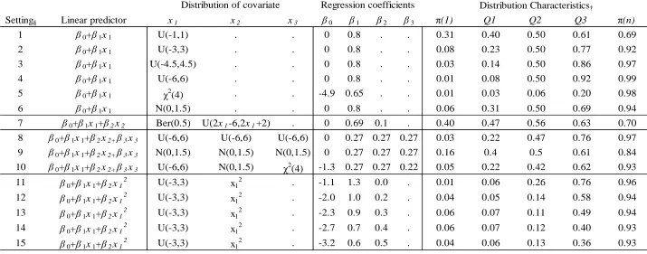
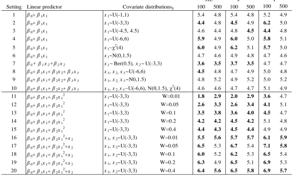
Table 4.1 Settings used to examine the null distributions and the power of HL, J2, and T. ... 73 Table 4.2 The linear predictors and distributional characteristics of the Stukel models used in

the power simulations. ... 74

Table 4.3 Summary statistics, rejection percentages, and Kolmogorov-Smirnov test results for

HL, J2 and T ... 80 Table 4.4 Simulated null rejection per cent† (n=100 and 500, r=10,000, α=0.05) for settings

1-24. ... 81

Table 4.5 Power of HL, J2 and T to detect a logistic model with an incorrectly specified linear predictor. ... 85

Table 4.6 Power of HL, J2 and T to detect a Stukel generalized model with an incorrectly specified logistic link function. ... 85

Table 5.1 General elements of the covariance matrix V, used in the calculation of TG, under the

logit, probit, log-log, complementary log-log, and log links. ... 98

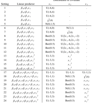
Table 5.2 (a-e) Settings for simulations used to investigate the null distributions of HL, J2 , and

T_G , and to evaluate the power of each statistic to detect an incorrectly specified link function. ... 109

Table 5.3 The distributional characteristics of the covariates and the linear predictors of the

settings used to examine the power of HL, J2, and T, to detect an incorrectly specified link function. ... 115

Table 5.4 Summary statistics, rejection per cent, and Kolmogorov-Smirnov test results for HL,

J2, and T_G. ... 125 Table 5.5(a-d) Simulated null rejection per cent (n=500, r=100,000, α=0.05). ... 130

Table 5.6 Empirical rejection per cent (α=0.05) when a model with a term omitted from the

linear predictor was fitted to data generated from a model with all terms. ... 137

Table 5.7 Empirical rejection per cent (α=0.05) when a model with an incorrectly specified link

(13)

(14)

List of Figures

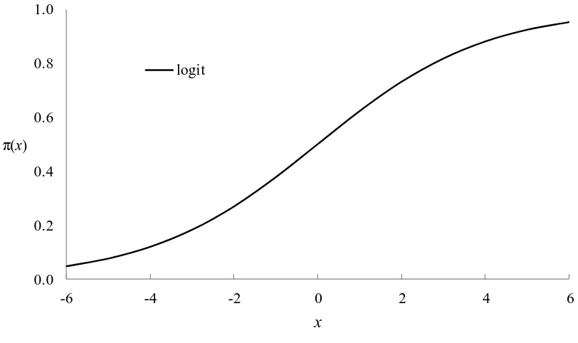
Figure 2.1 Graph of the probabilities produced by the inverse of the logit link function as a

function of x, where x~U(-6,6) and η=0.5x. ... 31

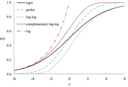
Figure 2.2 A graph of the probabilities produced by the inverse of five link functions as a function of x. (x~U(-6,6) and η=0.5x) ... 35

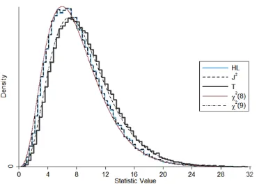
Figure 4.1 Histogram of 100,000 replications of setting 1. ... 79

Figure 4.2 Histogram of 100,000 replications of setting 5. ... 79

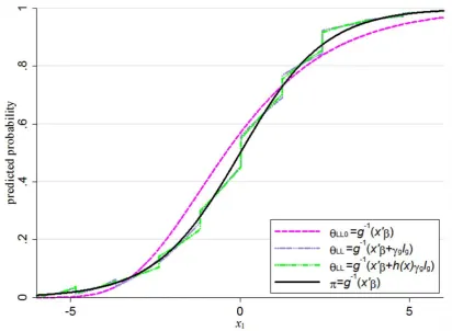
Figure 5.1 Graph of the predicted probabilities of a null log-log model (pink), an original Tsiatis log-log model (purple), a generalized Tsiatis log-log model (green), and the true logistic model (black) as a function of x. ... 103

Figure 5.2 Histogram of 100,000 replications of setting 3 using the probit link. ... 119

Figure 5.3 Histogram of 100,000 replications of setting 3 using the log-log link. ... 119

Figure 5.4 Histogram of 100,000 replications of setting 3 using the complementary log-log link. ... 120

Figure 5.5 Histogram of 100,000 replications of setting 3 using the log link. ... 120

Figure 5.8 Histogram of 100,000 replications of setting 10 using the complementary log- log link. ... 122

Figure 5.9 Histogram of 100,000 replications of setting 10 using the log link. ... 122

Figure 5.12 Histogram of 100,000 replications of setting 21 using the complementary log- log link. ... 124

(15)

Chapter 1 Introduction

“The oldest, shortest words – ‘yes’ and ‘no’ – are those which require the most thought.”

– Pythagoras

Yes or no, success or failure, life or death - these are all examples of binary responses. Critical

research questions can have answers that take this form. Once a scientist identifies such a

research question, designs a study, toils for hours collecting data, and then builds a regression

model appropriate for binary outcomes – after all of that, but before they can answer their

research question, they must first answer another binary question: ‘Does my model fit the data

that I observed?’ Their answer to this question will affect the conclusions they draw from all of

their hard work. It is critical. Checking the fit of binary regression models is central to this

thesis, and we began by giving a brief overview of the topic. Note that a more rigorous

explanation of the material in this overview will be given in Chapters two and three. We

conclude this introductory chapter with a list of the research questions that will be addressed in

the thesis, and give a synopsis of the thesis presentation.

1.1 Background

So how can the researcher decide whether or not to keep their model? One way is to calculate a

goodness-of-fit statistic that summarizes how well the outcomes predicted by their model fit the

outcomes they observed. This was the basic idea behind Karl Pearson’s well-known

goodness-of-fit test (Pearson 1900). Pearson is considered to be the “nucleus of the movement of

systematic statistical thinking”(Mukhopadhyay 2000). He was one of the first to introduce the

concept of goodness-of-fit. Originally he considered a multinomial variate with a fully specified

distribution function, whose range can be divided into some finite number of mutually exclusive

classes. Then, since the distribution function is specified, the probability of any observation

falling into a particular class can be calculated (Kendall, Stuart, Ord and Arnold 1999). One way

(16)

number of cells in a contingency table. Under the null hypothesis, the theoretical multinomial

probability of a being placed into a cell is equal to the probability derived from the observed

data and the parameters specified under the null hypothesis. The alternative is that they are

significantly different. Fisher extended Pearson’s work by considering the case when the

parameters are not fully specified (Kendall, et al. 1999). Later, Pearson’s test was applied to

regression models that can be fitted to obtain estimates of the parameters. This includes the

logistic regression model, which is used in many fields to relate a categorical outcome variable

to a set of predictor variables. It is a member of the class of models called generalized linear models (GLM), and can be used when the outcome data is assumed to come from a binomial distribution (McCullagh and Nelder 1989). If the outcome is binary, then it comes from the

Bernoulli distribution, which is a special case of the binomial distribution. In regression models,

the characteristics that correspond to the cells in the contingency table are the “covariate

patterns”. These are the unique combinations of the possible categories created by the covariates

in the model. For instance, if there were two covariates, say gender and smoking status, the

covariate patterns would be: male smoker, female smoker, male non-smoker, female

non-smoker.

Pearson’s test is usually called Pearson’s chi-squared test, and the test statistic often represented

by _X2_{. The name describes the distribution of the statistic. Pearson proved that, given a single}

variate with some fixed number of exclusive classes, the asymptotic distribution of the statistic

is chi-squared, with degrees of freedom equal to the number of classes, minus one. In the case

when there is more than one variate, then the degrees of freedom are calculated by determining

the number of classes for each variate, subtracting one from each, and then taking the product.

Pearson only considered the case when all parameters are specified. R.A. Fisher extended _X2_to

situations where parameters are unspecified. He proved that, in the case of a single variate, the

distribution then is asymptotically chi-squared with degrees of freedom equal to the number of

possible response types, minus the number of estimated parameters, minus one.

(17)

In order for the distributional properties of _X2_{to hold, there must be enough data in each cell}

of the contingency table, or likewise with every particular covariate pattern. If there are too few

observations of this type recorded, then there is not enough information to estimate the binomial

probability for that particular pattern. In this case, the theory behind the asymptotic distribution

of _X2_{is not valid. For example, this happens when continuous data are included in a logistic}

regression model. In such cases, the number of covariate patterns may be as large as the number

of observations. Using 2

X in this situation is not appropriate (Kendall, et al. 1999, Hosmer and Lemeshow 2000).

A solution to this problem is to create artificial groups and apply a statistic similar to X2. That is, to form groups via a method that is based on more than just the natural groups formed by the

covariate patterns. Hosmer and Lemeshow (1980) were among the first to offer this type of

solution. Their statistic, denoted here as HL, uses a method that is based on ordering and placing into groups the predicted probabilities produced from the model. These are the

estimated probabilities that the outcome will occur, given the observed covariate data. The

number of groups will be denoted here as G. As a practical matter, they recommended creating ten groups and called the method “deciles-of-risk”. In practice though, other numbers of groups

can be used. Because these groups are created using the estimated parameters that reference all

of the data, which are random, the group boundaries are also random (Moore and Spruill 1975,

Kendall, et al. 1999). That is, the “cut-points” of the groups vary. This affects the distribution of

their statistic. Building on the work of others (Moore 1971, Moore, et al. 1975, Durst 1979),

Hosmer and Lemeshow determined that the approximate distribution of HL is 2



G2



. Although the Hosmer-Lemeshow test is popular, and widely cited in the literature, there have

been some difficulties reported. The value of HL calculated using a particular set of data can vary depending on the group boundaries chosen. Also, if tied values of the estimated

probabilities are not placed in the same group, different results can be obtained simply by

changing the order of the tied observations (Hosmer, Hosmer, Le Cessie and Lemeshow 1997,

(18)

the distributional assumptions may not be valid (Pigeon, et al. 1999a). Further, there are

typically multiple covariates in a model, and so observations are located in a multidimensional

coordinate system. The range of possible locations that any observation can take is within a

multidimensional volume. Because predicted probabilities are calculated as a single number, the

covariate vector corresponding to each observation in the covariate space is mapped onto a

single dimension, sometimes referred to as the “y-space”. This can cause problems (Kuss 2002).

Points that were far from each other in the volume of the multidimensional covariate space may

now be considered close in the single dimensional y-space. By reducing the multidimensional

information to a single dimension, the information about how the observations are related in

space will likely change, and some information about their original locations in the covariate

space will be lost.

A different solution proposed by Tsiatis (1980) involves a statistic, T, that is a quadratic form with a known asymptotic distribution (Halteman 1980, Tsiatis 1980). Rao (2002) defines a

quadratic form in n variables, x x₁, ₂,...,x_n, as the homogeneous quadratic function of the variables

1 1

n n ij i j i j

a x x  

 



x Ax (1.1)

where x



x x₁, ₂,...,x_n



is an n1 column vector and A is an nn symmetric matrix. Pearson’s statistic is a special case of the Tsiatis quadratic form.

Tsiatis approaches grouping differently than Hosmer and Lemeshow. His solution was to

partition the covariate space, thus retaining the original information about which observations

are “close” to one another. But there are also problems with this artificial grouping method.

There is no free lunch. One obvious problem is that there are many ways to partition the

covariate space, and choosing which to use is subjective. Different choices can give different

results (Su and Wei 1991). Here is another problem: consider a model containing many

covariates, say five. If the partition is performed so that each of these covariates is broken into

(19)

if the partitioning is any finer, the number of groups would increase rapidly. There are already a

relatively large number of groups, 25 32, created by the coarse partitioning. In order for these

groups to be populated sufficiently, for example with five observations each, at least 160

observations must exist. But that assumes that the distribution of observations among groups is

even. Since the data are sampled after partitioning and an even distribution cannot necessarily

be assumed, large amounts of data sufficient to populate these groups must be collected. This is

not ideal. An interesting side note about the Tsiatis test is that it was discovered simultaneously

by Halteman (1980), but Tsiatis published first. In his PhD thesis, Halteman gave a more

detailed analysis of the problem. He proved that T has a distribution that is 2



G1



, and that its distribution is unaffected when the group boundaries are created with a method that

references the data. He performed simulations to verify that the distribution of T was still approximately 2



G1



for finite data samples when the deciles-of-risk grouping method was used. He found that even though the grouping method referenced the data, the distribution was

essentially the same. His work, however, was not published.

Another statistic, one that combines properties of both HL and T, is one that was proposed by Pigeon and Heyse (1999b), and which they refer to as J2. This statistic is similar to HL, but multiplied by a “correction factor”. This results in a common numerator but differing

denominators between the two statistics. By multiplying by this factor, Pigeon and Heyse

account for variations between the predicted probabilities within the groups. They state that

many grouping methods can be used with their statistic, presumably without changing its

approximate 2



G1



distribution. They do not discuss how using grouping methods that reference the data, such as the deciles-of-risk, might affect the distribution of J2, though they apparently apply this method to _J2_{in an example where they compare}_HL_and_J2_.

When a new statistic is proposed, it is important to perform simulation studies to assess its

calibration and performance. Specifically, it is important to investigate whether the statistic

maintains the expected Type I error rate when a correctly specified model is applied to data, and

(20)

goodness-of-fit tests for logistic regression with continuous covariates, HL can be considered to be a kind of industry standard (Kuss 2002). When a new goodness-of-fit statistic for logistic

regression with continuous covariates is proposed in the literature, HL is often included in simulation studies to provide a comparison to the new statistic. However, to our knowledge, no

simulations studies have been published in the literature that compare HL, J2, and T. This leads to the first set of research questions addressed in this thesis.

1.2 Research Questions

The first set of research questions that are addressed in this thesis are:

If the deciles-of-risk grouping method is applied to J and to T , are their reported 2 distributions unaffected?

If the same grouping method (deciles-of-risk) is applied to HL , 2

J , and T , are there any differences in their performances? Specifically, do they all maintain the expected Type I error rate, and do they have similar power to detect incorrectly specified models?

A second set of research questions addressed in this thesis regards the application of HL, J2, and T to GLMs with binary outcomes other than the logistic regression model. The logistic model is the canonical GLM when the outcomes are assumed to come from a Bernoulli

distribution (McCullagh, et al. 1989). There are other models that can also be fit to Bernoulli

data, including the probit, the log-log, the complementary log-log, and the log binomial models.

These are all non-canonical GLMs (McCullagh, et al. 1989, Hardin and Hilbe 2007). These will

be described in more detail in Chapter 2. If any of these models are chosen to relate the outcome

and the covariates, the question still remains, “Does this model fit the data well?” Few

goodness-of-fit test statistics have been studied for these non-canonical GLMs. Some work has

been done, including a study by Blizzard and Hosmer (2006). They applied HL to the binary log binomial model. They wondered whether the distributional assumptions that apply when

(21)

that it could be applied, they concluded that more research was needed. This leads to the other

research questions addressed in this thesis. They are

Can HL , J , and T be used as goodness-of-fit test statistics for non-canonical GLMs 2 with Bernoulli outcomes? If so, what are their distributions under these models? If HL , J , and T are used as goodness-of-fit statistics for non-canonical GLMs with 2 Bernoulli outcomes and continuous covariates, are there differences in their

performances?

1.3 Organization of Thesis

This thesis is organized as follows: In Chapter two, necessary notation is introduced and

background concepts are discussed. Chapter three contains a review of the literature on

goodness-of-fit statistics for Bernoulli GLMs. Chapter four includes an analytical treatment and

a simulation study comparing the HL, 2

J , and T goodness-of-fit statistics in the logistic model setting when the deciles-of-risk grouping method is applied. An example comparing the

statistics in the logistic model setting is also presented. A new goodness-of-fit statistic for all

GLM with Bernoulli outcomes, based on T, is introduced in Chapter five, along with

corresponding forms of HL and T . In addition, a simulation study comparing the distributional characteristics and performance of the new statistic under the probit, log-log, complementary

log-log, and log binomial models is performed. Chapter five concludes with a real-world

example that illustrates the use of the three statistics under the four non-canonical link functions

studied. Finally, Chapter six contains an overall discussion of the research, including its

(22)

Chapter 2 Notation and Basic Concepts

2.1 Notation

First, we will set some notation to be used in the following chapters. Let Y



Y₁,...,Y_n





represent a column vector of n outcome random variables, and y



y₁,...,y_n



 represent the column vector of observed outcomes, which are realizations of Y. Assume further that the mean values of the components of Y, μ



₁,...,_n



, can be modelled with a function that depends on the values of K covariates and a constant. Consider n independent observations of the pairs



x_i,y_i



, i1,...,n, where, for the ithobservation, y_i is the observed outcome of the random variable Y_i, and x_i (x_i₀,x_i₁,...,x_iK) is a column vector of the observed covariate values, plus x_i₀1 to allow for the estimation of a regression constant. Let an n



K1



matrix X represent a design matrix, where each row contains the covariate data, x_i, for each of

the n observations. Finally, let β



 ₀, ₁,...,_K



 represent a column vector of regression coefficients. Other notation will be introduced within the text.

2.2 Generalized Linear Models

During the 20th century, several regression models were developed for the analysis of a variety

of data types, each requiring a different maximum likelihood algorithm for the estimation of

model coefficients and standard errors (Hardin, et al. 2007). Examples include the Gaussian or

normal model, the Poisson model, the probit model, and the logit model. The methods required

to estimate the parameters of some of these models are mathematically intensive. However, the

methods required to estimate the parameters of the Gaussian linear model, the Ordinary Least

Squares (OLS) method which has less restrictive assumptions than the maximum likelihood

methods, are relatively straightforward. Nelder and Wedderburn (1972) introduced the GLM

(23)

the relatively simple OLS methods for the estimation of model coefficients are extended to all

members of this class. The basic strategy of the GLM is to choose a link function that relates μ to a set of linear predictors, η



₁,...,_n



Xβ (McCullagh, et al. 1989). The following are assumed under GLM theory:

1) the components of Y are independently distributed, have means μ



₁,...,_n



, and each has a distribution in the exponential family;

2) there is a systematic component, η



₁,...,_n



Xβ, which is a column vector of linear predictors, with the ith element expressed as _ix β_i ; and

3) there is a monotonic, differentiable link function, g

 

 , that relates μ and η, such that, for the thi observation, g

 

_i _i

(McCullagh, et al. 1989).

2.3 Exponential Family

The outcomes modelled by GLMs are assumed to have distributions in the exponential family.

Some examples of exponential family distributions are the Gaussian, binomial, and Poisson. For

a distribution to be an exponential family member, it must be possible to express the probability

function of the outcome random variable, Y, in the form





 

; , exp ,

Y

y b

f y c y

a

 

  



  

 

 _  _

 

  (2.1)

where  is the canonical parameter, b

 

 is the cumulant function,  is the dispersion

(24)

of the GLM is the same function as the canonical parameter  , then   , and the link

function is referred to as the canonical link.

The exponential family of distributions have been historically popular partly because of their

many useful algebraic properties. One result of these properties is that the first derivative of the

log-likelihood function of each exponential family distributions results in an “observed minus

expected” form. Goodness-of-fit test statistics for regression models typically are based on the

comparison of the observed outcomes and the expected outcomes produced by the model, and

so GOF statistics can be developed that are based on the derivatives of the log-likelihood

functions of the exponential family distributions. We describe the general form of the likelihood

function for GLM here, as well as some identities that will be used later when discussing

GOF statistics.

The joint density function of an exponential family distribution for a set of outcomes y, given the canonical parameter and dispersion parameter, is expressed as





 





1

| , exp ,

n

i i i

i i

y b

f c y

a

 

  





  

 

 _  _

 

 



y (2.2)

since the observations are considered to be independent. The likelihood function is equal to the

probability density function, and has the same form as (2.2), but differs in that it conditions on

the observed data rather than on the parameters. That is, it indicates how likely it would be to

observe the sampled outcomes as a function of possible values of the canonical parameter,  ,

and . For n independent and identically distributed (i.i.d.) observations, the likelihood function is expressed as





1

, |

n

i i

L f   y





(2.3)

The log of the likelihood function, l, is often easier to work with mathematically. Assuming that the observations are i.i.d., the joint log likelihood for members of the exponential family is

(25)

 





1

,

n

i i i

i i

y b

l c y

a            _  _    



(2.4)

Next we present some of the identities that will be used later in the thesis. Their derivations can

be found in Kendall, et al. (1999) (section 17.14) and in Hardin, et al. (2007).

The mean or expected value of the first partial derivative of the log likelihood is

0 l E    _ _ 

  (2.5)

and 2 2 2 0 l l E    _ _ _ _   _ _    _ _    (2.6)

Assuming that the likelihood function is twice differentiable, differentiating both sides of (2.5)

and using (2.6), gives

2 ₂

2

var l E l l

       _    _     _  _  _      2 2 l E       _ 

  (2.7)

and 2 ₂ 2 l l E E   _ _ _  _ _ _  _{  } _   _          (2.8)

The left hand side of (2.8) is sometimes called the Fisher Information ((Kendall, et al. 1999)

Section 17.15).

Using (2.4), it can be shown (McCullagh, et al. 1989) that

 

i

_{ }

i i b E y        (2.9)

(26)

 

2

var

i

b y

a



  





  (2.10)

McCullagh, et al. (1989) note that because the term 2b

 

_i    depends only on the canonical parameter, and thus the mean, it is sometimes called the variance function and they

express (2.10) as var

 

 .

The chain rule can be applied to  l  to obtain the resulting score vector,



 l 0, l 1,..., l K



. Hardin, et al. (2007) show in detail that, for the kth regression coefficient, the score is

   

1 var

n

i i i

ik i

k i i

l y

x a

 

    

  

  

 _ _ 





_ __ _ (2.11)

They also show that if the link function chosen is the canonical link function, where   ,

then (2.11) simplifies to

 

1 n

i i

ik i

k

l y

x a



  

 

 _ 

 





_ _ (2.12)

Setting (2.11) to zero for each of the scores, results in K1 estimating equations. The roots of the K1 estimating equations can be used to estimate the values that maximize the log

likelihood function, and thus determine the maxima of the likelihood (Kendall, et al. 1999). The

maximum likelihood estimate of _kare expressed here as ˆ_k.

There are two main methods used to estimate the regression coefficients of GLM. We give a

brief overview here, but a more detailed discussion can be found in Hardin, et al. (2007). The

first is an iterative numeric search method called Newton-Raphson. When estimating the

regression coefficients, this method uses the Observed Information Matrix (OIM). The OIM is

the negative of the observed Hessian matrix. For the exponential family, the OIM has elements

(27)

 



 







 





 

2 2 1 ' 2 ₂ 2 2 ' 1 1 var var 1 1 var var n i i

k k i i

i i i

i i

i i i i k k

i l a y                      _ _  _    _ _   __ _ _   _ __ _ _ ___ _ _ _      _ _ _  _{ }_ __ __{ } _       



(2.13)

The covariance matrix of the model parameters is the inverse of the OIM. (Searle 2006, Hardin,

et al. 2007).

A second iterative numeric method for estimating the regression coefficients, due to Fisher, is

called “the method of scoring” or the iteratively reweighted least squares (IRLS) method

(Kendall, et al. 1999, Hardin, et al. 2007). In this case, instead of the OIM, the IRLS method

uses the expected information matrix (EIM), or Fisher information in (2.8). The EIM has

elements expressed generally as

 

2 2 1 ' ' 1 1 var n i

k k i i k k

l E a              _  _        _{ }  _  _ _    

 



_ _ (2.14)

When the link of the GLM is the canonical link function, that is when   , the matrices

(2.13) and (2.14) are equal, but this is not the case under non-canonical GLM.

Some test statistics, such as Rao’s efficient score test (Rao 2002), are based on the identities

(2.5) and (2.7). Goodness-of-fit statistics for canonical GLM can be developed from score tests

when the selected link function for the GLM is canonical, since then the estimating equations

reduce to the form (2.12). (McCullagh, et al. 1989, Kendall, et al. 1999). This is not the case

when the link function of the GLM is non-canonical.

2.4 GLM for Binary Data

Some of the most commonly used GLMs are those whose random components have binomial

distributions (Hardin, et al. 2007). We are primarily concerned with GLMs for binary outcome

data, and so first present here the properties of the binomial likelihood function that were

(28)

The probability mass function of the binomial distribution can be expressed as



| ,



n y



1



n y

f y n p p p

p



 

_{ } 

  (2.15)

where p is the probability of a successful outcome of an experiment and n is the number of times the experiment was performed. Because the binomial distribution is an exponential family

member, its distribution can be rewritten in the form of (2.1) as



| ,



exp ln ln 1





ln 1

n p

f y n p y n p

p p

    

 _ _ _   _{ }_

 _{ }

 

  (2.16)

In the case of the binomial distribution, the canonical parameter is

ln 1

p p

 _{ } _ 

  (2.17)

the cumulant function is b

 

  nln 1



p



, the dispersion parameter is 1, and the normalizing term is c y



,



0(McCullagh, et al. 1989). A special case of the binomial distribution, when n1, is the Bernoulli distribution.

The link function chosen, which relates a binomial random variable Y to a linear predictor , may be any suitable function that is monotonic and differentiable (McCullagh, et al. 1989).

However, if the canonical parameter of the exponential family is chosen as the link function it

leads to several desirable statistical properties, including relatively straightforward methods for

parameter estimation and methods for evaluating model fit. When Y comes from a Bernoulli distribution the canonical link function is the binary logit function,

 

ln 1

p p

 _{ } _



 

g (2.18)

(McCullagh, et al. 1989). In this case, as with all canonical link functions, g

 

 .

The mean and variance of y for GLM with Bernoulli outcomes can be obtained regardless of link function used, (Hardin, et al. 2007) by taking the first and second derivatives of the

(29)

b p   _  (2.19) and





2 1 b p p     

  (2.20)

Thus, as noted by Hardin, et al. (2007), unlike the linear model, when the random outcomes are

binomially distributed, the variance is related to the mean and thus is not constant, but varies

with the mean.

The Bernoulli probability density function expressed in canonical exponential form is



| ,



exp ln ln 1





1

p

f y y p

p

   _ _ _  _



 

  (2.21)

and the joint log likelihood in canonical form, is









1

; ln ln 1

1 n i i i i i p

l p y y p

p     _ _    



(2.22)

By (2.11), (2.19), and (2.20), the kth element of the score vector is





1 1

n

i i i

ki i

k i i i

l y p p

x p p           _ _ 





_  __ _ (2.23)

For Bernoulli outcomes, the general terms of the OIM, (2.13), are

























2 2 1 ' 2 ₂ 2 2 ' 1 1 1 1 1 2 1 1 n i i

k k i i i

i i

i i i

i i i i k k

i i

l p

p p

y p p

p p p p            _ _      _ _   __  _ _   __ _ _ ___ _ _ _      _  _  _{ }_ _ __ __{ } _        



(2.24)

and the terms of the EIM, (2.14), are





2 2 1 ' ' 1 1 n i i

k k i i i k k

l p E p p                   _ _  _ _    _  _ _ _ 

(30)

2.5 Canonical GLM for Bernoulli Outcomes (Binary Logistic

Regression)

Generalized linear models with Bernoulli outcomes and a canonical logit link function are

referred to as logit or logistic models. These are arguably the most commonly used models for

relating a binary outcome to a set of predictor variables (Hardin, et al. 2007). This model is

central to the discussion in Chapter 4 and Chapter 5, and we present the expressions necessary

for our discussion here.

Denoting the E Y



|x



for the logistic model as 

 

x , the canonical logit link function is then

 





ln

 

_{ }

1



 



 

 

 _ _



 

 

x x

x

g (2.26)

The inverse of the logit link function produces the mean, and is expressed as

 

_{ }

 

1 exp



 



 _ _

 x

g (2.27)

The canonical parameter, when the canonical logit link is chosen, is

 

ln

1



 



 

 

 _ _



 

 

x

x (2.28)

and its derivative with respect to  is

1

 

 

 _ _

  (2.29)

In the univariate case, when 

 

x is graphed as a function of x, a sigmoidal curve is produced that is symmetric about 0.5 . An example is shown in Figure 2.1. In the binary case, this

property allows for the code designation of one of the outcomes as a success and the other as a

(31)

0.0 0.2 0.4 0.6 0.8 1.0

-6 -4 -2 0 2 4 6

π(x)

x

[image:31.595.122.528.69.310.2]

logit

Figure 2.1 Graph of the probabilities produced by the inverse of the logit link function

as a function of

x

, where

x

~

U

(-6,6) and

η

=0.5

x

.

2.6 Non-Canonical Link Functions for Binary Outcomes

Generalized linear models with non-canonical link functions can also be used to relate outcomes

with Bernoulli distributions to a set of explanatory variables. We introduce several of these

models here, and the expressions necessary for the development of a goodness-of-fit test

statistic for non-canonical binary GLM presented in Chapter 5. In the previous section, the



|



E Y x under the canonical logistic model was expressed as 

 

x . When the link function is non-canonical, we will instead designate E Y



|x



generally as _G

 

x . When referring to the specific non-canonical probit, log-log, complementary log-log, and log models, we will replace

the subscript and denote the probabilities as _Pr

 

x , _LL

 

x , _Cll

 

x , and _LB

 

x respectively.

2.6.1 Probit

The probit model is a GLM with the non-canonical link function

 





1



 



Pr _Pr Pr

 _{ }  _

x x

(32)

where  is the cumulative normal distribution, expressed as

 

2

1 1

exp 2 2

v dv v dv

 

 



 

 

   _ _

 



(2.31)

Here,  3.1415..., and 

 

 is the probability density function of the standard normal

distribution (Hardin, et al. 2007).

The inverse of the link function giving E Y



|x



is

 

1

Pr Pr

  

 _{ } _ _x

g (2.32)

The canonical parameter under the probit model is

 



Pr Pr





 



ln 1 ln 1

   x  x       (2.33)

 



 



ln  1 



 

 

   

 _ _



  (2.34)

Like the logistic model, the probit model is symmetrical around a mean probability of 0.5, and

has a similar sigmoidal shape. An example when the inverse of the probit link for a univariate

model, E Y x



|



, is plotted against x is shown in Figure 2.2.

2.6.2 Log-log and Complementary Log-log

If the binary data to be analysed are unbalanced, that is, the number of 0s and 1s are unequal,

then either the log-log model or the complementary log-log model may be a better fit. If there

are many more 0s than 1s, then the log-log model may be the more appropriate model, whereas

if there are many more 1s than 0s, then the complementary log-log model may give a better fit

to the data. The E Y



|x



for these models is denoted here as _LL

 

x and _Cll

 

x respectively. The link functions for the log-log and complementary log-log models are

 

 _LL  ln



ln



_LL

 

x







g (2.35)

(33)

 

 _Cll ln



ln 1



_Cll

 

x







g (2.36)

respectively. The corresponding inverses of these link functions are

 



 



 

1

exp exp LL

LL      _ _ _ _{ } x g (2.37) and

 



 



 

1 _{1 exp} _exp

Cll Cll      _{ } _ _{ } x g (2.38)

The canonical parameters under the log-log and complementary log-log models are

 

ln 1 LL LL       _ _    x x (2.39)

and

 

ln 1 Cll Cll       _ _    x x (2.40)

respectively. Their derivatives with respect to  are

 



 



ln _LL 1 _LL

        _ _ _   x x



 



 

ln 1 LL LL      x x (2.41) and

 



 



ln _Cll 1 _Cll

        _ _    x x



 



 

ln 1 _Cll

Cll  



  x

x (2.42)

respectively.

These models produce asymmetric sigmoidal curves. The log-log curve has an elongated lower

(34)

the inverse of the log-log and the complementary log-log links for a univariate model, E Y x



|



, as a function of x are shown in Figure 2.2.

Because of the inherent asymmetry of these models, the coding of the model is not symmetric.

That is, the assignment of “success” and “failure” cannot be simply reversed (with just a sign

change). However the log-log and the complementary log-log make a complementary pair. That

is, the log-log model applied to outcomes y will give the same result as the complementary log-log model applied to 1y. Similarly, if the log-log is applied to 1 y, then the same result is obtained when the complementary log-log is applied to y.

2.6.3 Log Binomial

Another non-canonical GLM for binary data is the log model, also known as the log binomial

model. The E Y



|x



for the log binomial model will be denoted here as _LB

 

x . The link function for the log binomial model is the natural log function, and is expressed as,

 



_LB



ln



_LB

 



LB

 x   x 

g (2.43)

The inverse of the link function is

 

1

exp _LB

LB

  

 _ _

x

g (2.44)

The canonical parameter under the log binomial model is

 



 



ln _LB 1 _LB

  _ x  x _ (2.45)

 



 



ln _LB 1 _LB



 

 

 

 _ _



 

x x

 

1 1 _LB



 x (2.46)

(35)

greater than 1. An example of the graph of the inverse of the log link for a univariate model as a

[image:35.595.118.553.119.416.2]

function of x is shown in Figure 2.2.

Figure 2.2 A graph of the probabilities produced by the inverse of five link functions as

a function of

x

. (

x

~

U

(-6,6) and

η

=0.5

x

)

2.7 Basic Concepts of Score Tests

Some goodness-of-fit tests are formed as score tests. The score test statistic was introduced by

Rao (1948), and is based on the identities (2.5) and (2.6) (Smyth 2003). Suppose that the

likelihood function of a GLM, (2.4), depends on two vectors of parameters, and express this as



, |



l β γ y . The null hypothesis being tested is that γ 0, against the alternative hypothesis that  γ is unrestricted. Here, the β are considered nuisance parameters, while the γ are considered the parameters of interest. The column vector of scores can be partitioned as



,





 _β _γ

S S S (2.46)

(36)

l

 

 β

S

β (2.46)

and

l

 

 γ

S

γ (2.46)

The covariance matrix of the score vector (2.46) is the expected information matrix, I, with general elements as in (2.14). It can be partitioned to conform with (2.46) and (2.46), and

expressed as

 

  

 

ββ βγ

γβ γγ

I I

I

I I (2.47)

(Graybill 1976, McCullagh, et al. 1989). If the values of the nuisance parameters, β, are known, then the score test statistic, evaluated under the null hypothesis, is

 

1





γ γγ γ

γ 0

S I S (2.47)

(Smyth 2003). In this case, the score test statistic has a chi-squared distribution with degrees of

freedom equal to the rank of I_γγ(Rao 2002).

If the nuisance parameters are not known, then the maximum likelihood estimates under the null

hypothesis, ˆβ, are substituted. Using the multivariate theory on inverses (Graybill 1976, McCullagh, et al. 1989), the covariance matrix, conditional on β = βˆ₀, is

1 ˆ

|



 γγ  γβ ββ βγ γ β

I I I I I (2.48)

(McCullagh, et al. 1989, Smyth 2003).

The score test statistic in this case is calculated as

 

1 ˆ

| _ˆ

,



 



γ γ β γ

γ 0 β β

(37)

where all of the terms of the statistic are evaluated under the null hypothesis γ 0 , and under ˆ



β β. Here, the score test statistic has a distribution that is asymptotically chi-squared with degrees of freedom equal to the rank of I_{γ β}_|_ˆ(Rao 2002) . If I_βγ 0, then β and γ are

(38)

Chapter 3 Literature Review

3.1 Goodness-of-Fit Statistics for Binary Logistic Regression

Models

After selecting the explanatory variables to include in a binary logistic regression model and

determining an appropriate mathematical function that best describes an “average” value of the

outcome variable for the given covariate values, a critical next step in model development is to

examine whether the predicted probabilities calculated from the chosen model and covariates

are significantly different from the observed outcome values. That is, does the model fit the

observed outcome data well? Goodness-of-fit statistics are used to test the hypothesis that the

distribution function of the observed outcome variable is the same as the distribution function of

the hypothesized model (Kendall, et al. 1999). Two types of goodness-of-fit tests, specific and

global, are used to test this null hypothesis (Kuss 2002). The specific test is used to test the null

against the alternative that that another specific model would fit the data better. The global test

does not evaluate a specific alternative, but rather tests against the alternative that the model

does not fit, without specifying in what way the fit may be poor. The focus of this thesis is on

global GOF tests. Two well-known global test statistics used to assess the fit of binary logistic

regression models are the deviance and the Pearson’s chi-square.

3.1.1 Deviance

The deviance is a likelihood ratio test that compares the fits of two models to the observed data;

the first is the null model which is under consideration, and the second is a saturated model in

which the null model is nested. The saturated model includes a parameter for each of the J

covariate patterns. The hypothesis being tested is that all parameters of the saturated model that

are not in the working model are equal to zero. In this section we will refer generally to the

estimated probabilities of the binary model as ˆ , for ease of notation. The deviance residual

Grouped goodness of fit tests for binary regression models