MoL 2015 13: Computable Analysis Over the Generalized Baire Space

Computable Analysis Over the Generalized Baire Space

MSc Thesis

(Afstudeerscriptie)

written by

Lorenzo Galeotti

(born May 6th, 1987 in Viterbo, Italy)

under the supervision of Prof. Dr. Benedikt L¨owe andDrs. Hugo Nobrega, and submitted to the Board of Examiners in partial fulfillment of the requirements for the degree of

MSc in Logic

at theUniversiteit van Amsterdam.

Date of the public defense: Members of the Thesis Committee:

July 21st, 2015 Dr. Alexandru Baltag (Chair)

Contents

1 Introduction 1

2 Basics 4

2.1 Orders, Fields and Topology . . . 4

2.2 Groups and Fields Completion . . . 7

2.3 Surreal Numbers . . . 10

2.3.1 Basic Definitions . . . 10

2.3.2 Operations Over No . . . 13

2.3.3 Real Numbers and Ordinals . . . 15

2.3.4 Normal Form . . . 16

2.4 Baire Space and Generalized Baire Space . . . 17

2.5 Computable Analysis . . . 19

2.5.1 Effective Topologies and Representations . . . 19

2.5.2 Subspaces, Products and Continuous Functions . . . 21

2.5.3 The Weihrauch Hierarchy . . . 22

3 Generalizing R 24 3.1 Completeness and Connectedness ofRκ . . . 24

3.2 κ-Topologies . . . 26

3.3 Analysis Over Super Denseκ-real Extensions ofR . . . 29

3.4 The Real Closed Field_Rκ . . . 32

3.5 Generalized Descriptive Set Theory . . . 42

4 Generalized Computable Analysis 52 4.1 Wadge Strategies . . . 52

4.2 Computable Analysis Overκκ_{. . . . 54}

4.3 Restrictions, Products and Continuous Functions Representations . . . 58

4.4 Representations forRκ . . . 63

4.5 Generalized Choice Principles . . . 68

4.6 Baire Choice Functions . . . 76

4.7 Representation of the IVT . . . 79

5 Conclusions and Open Questions 85 5.1 Summary . . . 85

5.2 Future Work . . . 86

Abstract

One of the main goals of computable analysis is that of formalizing the complexity of theorems from real analysis. In this setting Weihrauch reductions play the role that Turing reductions do in standard computability theory. Via coding, we can transfer computability and topological results from the Baire spaceωω to any space of cardinality 2ℵ0, so that e.g. functions overR can be coded as functions over the Baire space and then studied by means of Weihrauch reductions. Since many theorems from analysis can be thought to as functions between spaces of cardinality 2ℵ0, computable analysis can then be used to study their complexity and to order them in a hierarchy.

Recently, the study of the descriptive set theory of the generalized Baire spaces κκ _{for cardinalsκ > ω}

has been catching the interest of set theorists. It is then natural to ask if these generalizations can be used in the context of computable analysis.

In this thesis we start the study of generalized computable analysis, namely the generalization of com-putable analysis to generalized Baire spaces. We will introduce _Rκ, a Cauchy-complete real closed field of

cardinality 2κ _{withκ uncountable. We will prove that}

Rκ shares many features with R which have a key role in real analysis. In particular, we will prove that a restricted version of the intermediate value theorem and of the extreme value theorem hold inRκ.

We shall show that Rκ is a good candidate for extending computable analysis to the generalized Baire

spaceκκ_{. In particular, we generalize many of the most important representations of}

RtoRκ and we show

that these representations are well-behaved with respect to the interval topology overRκ.

Chapter 1

Introduction

Computable Analysis

Computable analysis is the study of the computational properties of real analysis. We refer the reader to [28] and [6] for an introduction to classical computable analysis.

In classical computability theory one studies the properties of functions over natural numbers and then transfers these properties to arbitrary countable spaces via coding. The same approach is taken in computable analysis.

One of the main tools of computable analysis is the Baire space ωω_{, namely the space of sequence of}

natural numbers of length ω. Following the classical computability theory approach, computational and topological properties ofωω _{are studied and then transferred to spaces of cardinality 2}ℵ0 _{via coding.}

Roo

Coding

ωω

Of particular interest in computable analysis is the study of the computational and topological content of theorems from classical analysis. The idea is that of formalizing the complexity of theorems by means similar to those used in computability theory to classify functions over the natural numbers. In this context, the Weihrauch theory of reducibility plays a predominant role. For an introduction to the theory of Weihrauch reductions see [5]. Weirauch reductions can be used to classify functions over the Baire spaceωω_{. Intuitively,}

a functionf :ωω_→ωω_{is said to be Weihrauch reducible tog:ω}ω_→ωω_{if there are two continuous functions}

which translatef intog as shown in the following commuting diagram:

ωω

f

Input Translation _//

ωω

g

ωωoo Output Translation _ωω

Many theorems from classical analysis can be stated as formulas of the type:

∀x∈X∃y∈Y. ϕ(x, y),

with ϕ a quantifier-free formula. These formulas can be formalized by using multi-valued functions. A multi-valued functionT :X _⇒Y is a function that given an elementxof X returns a subset ofY. Let us consider two classical examples, namely the Intermediate Value Theorem and the Baire Category Theorem.

The statement of the Intermediate Value Theorem is the following:

where C[a,b] is the set of continuous functionsf : [a, b]→Rsuch thatf(a)·f(b)<0. We can formalize this formula by the following multi valued function:

IVT : C[a,b] ⇒[a, b],

where, given a functionf ∈C[a,b], the set IVT(f)⊂[a, b] is such that

c∈IVT(f)⇒f(c) = 0.

The Baire Category Theorem can be stated as follows:

Given a countable sequence of closed nowhere dense subsets (An)n∈ω of a complete separable metric space

X, the setX\S

n∈ωAn is not empty.

Therefore it can be formalized by the following multi valued function:

BCT :A(X)N_⇒X,

whereA(X)N _{is the set of the countable sequences of closed nowhere dense subsets ofX. Given a sequence}

(An)n∈ω, we have that:

BCT((An)n∈ω)∈X\

[

n∈ω

An.

The previous two examples show that even though both the Intermediate Value Theorem and the Baire Category Theorem have a similar logical form, the multi-valued functions that represent them are quite different. It seems then really impractical to compare these two multi-valued functions directly. This apparent difficulty can be overcome by using the Baire space.

A multi-valued function T : X _⇒ Y is usually coded within the Baire space as the set of functions

t :ω →ω such that for every p∈ωω_{, we have that C(f(p))∈T(C(p)) where C is the function codingX}

in ωω_{. Given two multi-valued functions T}

1 :X1 ⇒Y1 andT2 :X2 ⇒Y2 one can therefore compare their

complexity by studying the Weihrauch reducibility of their codings. In particular, one can study what is the relationship, with respect to Weihrauch reducibility, of the representations ofT1andT2. For this reason

it is natural to use the Weihrauch theory of reducibility to compare theorems from analysis. The following diagram illustrates the situation for IVT and BCT:

C[a,b] IVT o o Coding ωω Translation + + k k Translation ivt ωω bct

Coding _//

A(X)N

BCT

[a, b]oo

Coding ω ω Translation + + k k Translation ωω

Coding //X

By using this technique it is possible to arrange many theorems from classical real analysis in a complexity hierarchy called the Weihrauch hierarchy. A study of the Weihrauch degrees of the most important theorems from real analysis can be found in [5] and [2].

Generalized Baire Spaces

Recently, generalizations of the Baire space to uncountable cardinals have been of great interest for descriptive set theorists. We refer the reader to [13] for an introduction to generalized descriptive set theory. Even though the theory of generalized Baire spacesκκ_{withκuncountable is not a new concept in set theory, many aspects}

of this theory are still unknown. In particular it is still unclear how these generalizations can be used in the context of computable analysis.

In this thesis we will begin for the first time the study of generalized computable analysis, namely the generalization of computable analysis to generalized Baire spaces. Given a space M of cardinality 2κ_{, the}

idea is that of substituting the Baire space ωω _{with the generalized Baire space κ}κ _{and then of developing}

the machinery necessary in order to transfer topological properties formκκ _{to M. In particular we will be}

interested in the study of the Weihrauch hierarchy in the context of generalized Baire spaces.

What is the right generalization ofRin the context of generalized computable analysis?

R

Generalization

o

o Coding

ωω

Generalization

?oo Coding κκ

One of the main results of this thesis is the definition ofRκ, a generalization of the real line which provides a

well-behaved environment for generalizing real analysis and for developing generalized computable analysis.

Generalizations of the Real Line

The problem of generalizing the real line is not new in mathematics. Different approaches have been tried for very different proposes. A good introduction to these numbers systems can be found in [12]. Among the most influential contributions to this field particularly important are the works of Sikorski [26] and Klaua [18] on thereal ordinal numbers and that of Conway [9] on thesurreal numbers. Sikorski’s idea was to repeat the classical Dedekind construction of the real numbers starting from an ordinal equipped with the Hessenberg operations (i.e., commutative operations over the ordinal numbers). Later Klaua extended Sikorski’s work providing a complete study of this number system. Unfortunately the real ordinal numbers do not behave well in terms of analysis. In particular one can prove that these fields do not have the density properties that, as we will see, will have a central role in this context.

The surreal numbers were introduced by Conway in order to generalize both the Dedekind construction of real numbers and the Cantor construction of ordinal numbers. In his introduction to surreal numbers, Conway proved that they form a (class) real closed field (i.e., they have the same first order properties as the real numbers). Later, Dries and Ehrlich [18] proved that every real closed field is isomorphic to a subfield of the surreal numbers, showing therefore that they behave like a universal (class) model for real closed fields. It is then natural for us to use this framework in the development of_Rκ.

Our Results

As we will see, doing analysis over field extensions of_Ris not an easy task. In particular, this is due to the fact that no proper ordered field extension of_Ris connected. Intuitively this means that no such extension can be a linear continuum in the topological sense, namely it has many holes that can be detected by the interval topology. This is of course a problem if we want to do real analysis because many basic theorems of real analysis are in fact strongly related, sometimes even equivalent, to the fact thatRis a connected space. To overcome this problem, instead of using standard topological tools, we will use a different mathematical framework which, under specific conditions over the density ofRκ, will allow us to see our field extension of

R as a linear continuum. By using these tools, we will prove some basic facts from classical analysis over Rκ. In particular, since the Intermediate Value Theorem and the Extreme Value Theorem are two of the

pillars of real analysis on which many others concepts rely, we will place particular attention on them. The second part of this thesis will be devoted to the study of generalized computable analysis. In particular we will generalize the standard machinery from computable analysis by using generalized Baire spaces. Then we will start the study of_Rκ from a computable analysis point of view, showing that, because

of its properties,_Rκfits perfectly the role of extension ofRto the generalized Baire spaceκκ. In particular we will show that many of the classical codings of_Rgeneralize naturally to_Rκ.

In the last part of this thesis, we will use all of the generalized tools we have developed to start the study of the Weihrauch hierarchy over_Rκ. We will show that some results from classical Weihrauch theory

can be carried over to_Rκ andκκ. In particular we will generalize some of the choice principles introduced

Chapter 2

Basics

Before we start with the basic notions we will need to develop our theory of generalized computable analysis, we want to stipulate the following convention:

In this thesis, κ will refer to a fixed cardinal larger than ω. Moreover, since we are extending R to the generalized Baire space κκ_{, we will assume κ}<κ _{= κ. This is a standard requirement in generalized}

descriptive set theory. Moreover, since one of the essential features of ω that makes computable analysis work is thatω<ω=ω, it is natural for us to assume1:

ASSUMPTION:κ<κ =κ.

2.1

Orders, Fields and Topology

Orders, ordered fields and topologies will be central concepts all over this thesis. In this section we will recall some of the basic definitions and properties of ordered sets, ordered fields and topological spaces. We start with the definition of partial order:

Definition 2.1.1(Partial Order). Let P be a set and ≤be a binary relation overP such that: • ∀p∈P. p≤p(Reflexivity).

• ∀p, q∈P. p≤q∧q≤p⇒p=q (Antisymmetry). • ∀p, q, z∈P. p≤q∧q≤z⇒p≤z (Transitivity). then(P,≤)is called a partial order. Moreover if

∀p, q∈P. p≤q∨q≤p∨p=q,

then(P,≤)is called a total(or linear) order. A totally ordered subset of a partial order is called a chain.

As usual if p, q ∈P are such that p≤q andp6=q then we will write p < q (pis strictly smaller than

q). Given two subsets A and B of a partial order (P,≤) we use the convention of writing A < B if every elementa∈A is strictly smaller than every element ofB.

Definition 2.1.2. Let (P,≤)be a totally ordered set andA be a subset ofP. Then we have: • P is denseiff∀p, q∈P. p < q⇒ ∃r∈P. p < r < q.

• A⊆P is dense inP iff∀p, q∈P. p < q⇒ ∃a∈A. p < a < q. • A⊆P is cofinalin P iff∀p∈P.∃a∈A. p≤a.

• A⊆P is coinitialin P iff∀p∈P.∃a∈A. a≤p.

We will call cofinalityofP the smallest cardinalκ0 such that there is a cofinal subset ofP of cardinality κ0. We will denote the cofinality ofP withCof(P). Similarly, we will call coinitialityofP the smallest cardinal

κ0 _{such that there is a coinitial subset ofP of cardinality κ}0_{. We denote the coinitiality ofP with Coi(P).} Finally we will call weight of P, w(P) the smallest cardinal κ0 such that there is a dense subset of P of cardinality κ0.

Let us illustrate this notions by using a familiar example. Let_Rbe the set of real numbers endowed with the usual order. Then (_R,≤) is a total order and _Q, the set of rational numbers, is dense in _R. Moreover N, the set of natural numbers, is cofinal in R but is not coinitial, while Z, the set of integer numbers, is both cofinal and coinitial in R. As one can imagine cofinality, coinitiality and weight are three important properties of an ordered set, and as we will see they will be central in most of our constructions.

Definition 2.1.3. Let (P,≤) be a totally ordered set. Then a sequence over P is an injective function

S = (xi)i∈α whose domain is an ordinal αand codomain is P. αis the length of s and will be denoted as

|S|. A sequence is strictly increasingif for allγ, β < α, such thatγ < β thenxγ < xβ. Similarly, a sequence

is strictly decreasingif for all γ, β < α, such thatγ < β we have xβ< xγ.

Definition 2.1.4. Let (P,≤) be a total order, α and β be two ordinals, s1 = (xi)i∈α and s2 = (yi)i∈β be

two sequences over P. Then we define:

• forγ < α,s1γ= (xi)i∈γ, the restrictionofs1 toγ.

• Forp∈P,s_

1 p= (xi)i∈α+1 wherexα=p, the extensionofs1 byp. More generally we defines_1 s2as

the concatenation of s1 ands2. We will sometimes omit the symbol_, writings1s2 instead ofs_1 s2.

• s1⊆s2 iff there isγ < β such thats1=s2γ, in this case we say thats1 is a prefix ofs2.

• s1/ s2 iff there are γ < β such that for all i <|s1|,xi =yγ+i, namely ifs1 is a subsequence ofs2.

Let us illustrate the previous concepts with an example.

Example 2.1.5. Let α be an ordinal and {0,1}<α _{be the set of sequences with domain in κ. We have}

0011010 ∈ {0,1}<α _{and the sequence1}

β of β ones is in {0,1}<α if β < α. Then 0011010_1β ∈ {0,1}<α

is the sequence 0011010 followed byβ ones. We have that 00⊂0011010,1 6⊂0011010, 101/0011010 and

111₆0011010.

Now we will recall two fundamental properties of orders introduced by Hausdorff, which will become extremely important later in this thesis.

Definition 2.1.6. Let (P,≤)be a totally ordered set andκ0 be a cardinal. Then we have:

• P is an ακ0-set iff every subset ofP has a cofinal and coinitial subset of cardinality less than κ0.

• P is an ηκ0-set iff givenL, R⊆P, such that L < R and|L|+|R|< κ0 then there isx∈P such that

L <{x}< R.

In particular ηκ0-sets for κ0 uncountable are interesting. Intuitively a set X is an η_κ0-set if it is very dense, namely if in order to find an hole in the space unbounded sets of cardinality at leastκ0 are necessary. Now that we have introduced all the basic definitions about orders we can start considering ordered groups and fields. We refer the reader to [8] for a complete introduction to field theory. We will recall some definitions that will be important in this thesis.

Definition 2.1.7 (Ordered Group). Let (G,+,0) be a group and < be an order relation over G. Then

(G,+,0, <)is an ordered group iff

∀a, b, c∈G. a≤b⇒a+c≤b+c.

Let us illustrate these notions by two examples. The integers endowed with classical order and addition form an ordered group. Note, thatZ+has a minimum (i.e., 1), therefore Deg(Z) = 1. The rational numbers with their standard order and addition also form a group of degree ω. It is easy to see that the sequence (1

n)n∈ωis coinitial inQ

+_{. Moreover, by the density of}

Qfor every finite sequence of positive rational numbers (qn)n<m there is q∈Qsuch that

0< q <{qn |n < m},

therefore (qn)n<m can not be coinitial inQ+.

Given an ordered group we can define theabsolute value ofa∈Gas follows:

|a|=

(

a ifa≥0

−a otherwise.

It is easy to see that

|a+b| ≤ |a|+|b|

for everya, b∈G.

Definition 2.1.8 (Ordered Field). Let (K,+,0,1,·) be a field and < be an order relation over K. Then

(K,+,·, <)is an ordered field iff: • (K,+, <)is an ordered group.

• For every a, b∈K bigger than 0,0≤a·b.

Using this definitions is not hard to see that many of the inequalities used in algebra hold for ordered fields. For example we have the following:

• 0<1.

• For alla, b, c∈K,a < bandc >0 impliesa·c < b·c.

• For alla∈K,a <0 implies−a >0.

• For alla, b, c∈K,a < bimpliesb−a >0.

• For alla, b∈K,a < banda, b >0 impliesa−1_{> b}−1_.

The most important examples of ordered fields are the set of rational numbersQand the set of real numbers Rendowed with the standard ordering and operations. As we said in the introduction one of the main aim of this thesis is that of finding a generalization of the field of real numbers which can be used in the context of computable analysis over the generalized Baire spaceκκ. It is natural then to focus on those fields which have the same (first order) properties ofR. Fields of this kind, form a special subclass of fields:

Definition 2.1.9 (Real Closed Field). A field K is real closed if every positive a∈ K is a square and if every polynomial of odd degree with coefficients inK has a root.

It is a well known fact that the theory of real closed fields in the language (+,·,0,1, <) is model complete (i.e. every embedding of real closed fields is elementary). In particular it is easy to see that since the theory of real closed fields is model complete, every real closed fieldK is elementary equivalent to _R. In fact, let

K be a real closed field. SinceK has characteristic zero, _Qis embedded in K. Therefore, the field of real algebraic numbers is an elementary submodel ofK(note that the real algebraic numbers are the smallest real closed field containing _Qsee [19]). Now, since the field of real algebraic number is known to be elementary equivalent toR(see [20]), all the first order properties ofRtransfer toK. In particular this implies that the theory of real closed fields is complete. We refer a reader interested to the model theory of real closed fields to [20].

We conclude this section by recalling some basic notions from topology which will be particularly impor-tant for our constructions. We will use definitions and terminology from [22]. First recall that a topological space (X, τ) is T0 if for everyx, y∈ X there is an open set U ∈ τ such thatx∈U and y /∈U, is second

The order on Rand the topology induced by this order have a central role in this field. Let (X,≤) be an ordered set. Theinterval topology over X is defined as the topology generated by the baseB defined as follows:

• (a, b)∈B for every a, b∈X such thata < b.

• Ifb0is the maximum inM, then (a, b0]∈B for everya∈X.

• Ifa0 is the minimum inM, then [a0, b)∈B for every b∈X.

The most important example of order topology is the topology on_Rgenerated by the open intervals of real numbers.

Another topology which will have a relevant role in our constructions is the subspace topology. Given a topology (X, τ) and a subsetY ofX we define the subspace topology overY as follows:

τY ={U∩Y |U ∈τ}.

Naturally we have that the base ofY is related to that ofX.

Lemma 2.1.10. Let (X, τ)be a topology, B be a base ofτ andY ⊂X. Then

BY ={B1∩Y |B1∈B},

is a base for the subspace topology.

Finally, letY be a set, (X, τ) be a topological space andf :X →Y be a surjective function. Then the

final topology induced byf is defined as follows:

O∈τ iffδ−1[O] is open in dom(f).

Note that sinceδis surjective and continuous with respect to the final topology, then it is a quotient map. As we will see final topologies will have a central role both in classical and in generalized computable analysis.

2.2

Groups and Fields Completion

In this section we will recall some basic facts about group and field completions. A complete treatment of these subjects can be found in [8] and [10]. All the results in this section can be found in [10]. First we will present a general construction ofcut completion over a groupG.

Definition 2.2.1. Let Gbe a totally ordered group andL, R⊆Gbe subsets ofGsuch that

L < R.

We will callhL, Ria cutoverG.

Definition 2.2.2. Let Gbe a totally ordered group and C the set of all the cuts over G. Then we say that

Gis C-complete iff for everyhL, Ri ∈C there is x∈Gsuch that L <{x}< R.

Now we will define a general procedure which given a totally ordered dense group Gand its set of cuts

C, constructs a groupGC which containsGand isC-complete. First we define an order relation over Cas follows:

hL1, R1i ≤ hL2, R2i ⇔ ∀`1∈L1∃`2∈L2. `1≤`2.

We define an equivalence relation∼overC as follows:

hL1, R1i ∼ hL2, R2i ⇔ hL1, R1i ≤ hL2, R2i ∧ hL2, R2i ≤ hL1, R1i.

First of all note that for allx∈Gwe can define a cuthLx, Rxiby taking

Lx={y∈G|y < x}

and

Rx={y∈G|y > x}

Then the mappingx7−→[hLx, Rxi] is an embedding ofGin GC.

It is easy to see that, if we define the order onGC as follows:

[hL1, R1i]≤[hL2, R2i]⇔ hL1, R1i ≤ hL2, R2i,

then the embedding preserves the order.

We define the addition overGC in the following way:

[hL1, R1i] + [hL2, R2i] = [hL1, R1i+hL2, R2i],

wherehL1, R1i+hL2, R2iis defined as follows:

hL1, R1i+hL2, R2i=h{`1+`2|`1∈L1, `2∈L2},{r1+r2|r1∈R1, r2∈R2}i.

It is not hard to see that the embeddingx7−→[hLx, Rxi] also preserves +. Indeed:

[hLx+y, Rx+yi] = [hLx+Ly, Rx+Ryi] = [hLx, Rxi] + [hLy, Ryi].

It is then clear thatGC _{is a totally ordered group. Finally we claim that G}C _{is complete. Let hL, Ribe in}

C. Then defining

L0= [

[hLα,Rαi]∈L

Lα

and

R0= [

[hLα,Rαi]∈R

Rα,

we have thatL <[hL0, R0i]< RinGC_{. ThereforeG}C _{is complete.}

Now, if G is an ordered field we can extend this completion in such a way thatGC _{is also an ordered}

field. We only need to define the multiplication over GC_{. Letx, y∈G}C _{with x, y >0,x= [hL}

x, Rxi] and

y= [hLy, Ryi]. Then we define:

x·y= [hLx, Rxi · hLy, Ryi],

wherehLx, Rxi · hLy, Ryiis defined as follows:

hLx, Rxi · hLy, Ryi=h{`x·`y|`x∈Lx, `y∈Ly},{rx·ry|rx∈Rx, ry∈Ry}i.

Moreover we define:

x·y=

        

(−x)·(−y) iffx, y <0,

−((−x)·y) iffx <0 y >0,

−(x·(−y)) iffx >0 y <0,

0 iffx= 0 ∨ y= 0.

Note that, ifGis a real closed field, thenGC _{endowed with· fulfils all the properties of a real closed field,}

and thatx7−→[hLx, Rxi] is a field morphism betweenGandGC (see [10]).

Definition 2.2.3. Let K be an ordered field and C the set of cuts over K. Then K0 _{is a C-completion of}

K if it is C-complete andK is isomorphic to a dense subfield of K0.

By what we have just seen we have:

Theorem 2.2.4. Let K be an ordered field and C the set of cuts over K. Then KC is a C-completion of

L R

ε

{

Figure 2.1: A Cauchy cut.

Now note that the previous construction is a generalization of the classical Dedekind construction of the real numbers. In particular by taking G =_Q and restricting C to the set of Dedekind cuts over _Q (i.e., imposingL 6=∅ and R6=∅ for every hL, Ri ∈ C), we have that GC ₌

R. Now we want to show that the classical Cauchy completion of a field is also just a particular case of the previous construction.

Definition 2.2.5(Cauchy cuts). Let Gbe a totally ordered group and hL, Ribe a cut overG. We will say that hL, Riis a Cauchy cut iff it is a cut such that,L has no maximum, R has no minimum and for each

ε∈G+ _{there are `∈L andr∈R such that r < `+ε. We will say that Gis Cauchy-completeiff for each}

Cauchy cut hL, Ri, there isx∈Gsuch thatL <{x}< R.

Intuitively Cauchy cuts are cuts whose elements of the left and right sets get arbitrarily close to each other (Fig.2.1).

Definition 2.2.6. Let K be an ordered field. We will say that K0 is a Cauchy cut completion of K iffK

is a dense subset ofK0 andK0 isC-complete withC set of Cauchy cuts over K0.

Theorem 2.2.7. Let K be a field and C be the set of Cauchy cuts over K. Then KC is a Cauchy cut completion of K.

Proof. The construction of KC _{we have just defined works perfectly also with C restricted to the set of}

Cauchy cuts overK.

Classically a Cauchy completion of an ordered field is characterized in terms of sequences as follows:

Definition 2.2.8(Cauchy sequences). LetGbe a totally ordered group, andαan ordinal. Then a sequence

(xi)i∈α of elements of Gis Cauchyiff:

∀ε∈G+∃β < α∀γ, γ0≥β. |xγ0−x_γ|< ε.

The sequence is convergentif there isx∈Gsuch that:

∀ε∈G+∃β < α∀γ≥β. |xγ−x|< ε.

We will call x the limit of (xi)i∈α. Given a group G it is said to be Cauchy complete iff every Cauchy

sequence of lengthDeg(G)has a limit inG.

It turns out that being Cauchy cut complete and being Cauchy complete are is equivalent notions.

Proposition 2.2.9 (Dales & Woodin). Let hL, Ri a Cauchy cut in an ordered group G. Then |L| = Deg(G) =|R|.

Proof. See [10, Proposition 3.3]. Then we have the following:

Theorem 2.2.10 (Dales & Woodin). The group Gis Cauchy cut complete iffGis Cauchy complete. Proof. AssumeGCauchy cut complete, and let (xi)i∈αbe a Cauchy sequence inG. For each ε∈G+ there

isσε>0 such that for everyi, j≥σε, we have|xi−xj|< ε. Define

and

R=[{([xσε+ε,+∞)|ε∈G

+

}.

Then for everyε ∈G+ _{take 0< ε}0 _{< ε, then take` ∈L, r ∈R such that `=x}

σ_ε0 −ε

0 _{and r =x}

ε0+ε0, then`+ε > r. HencehL, Riis Cauchy and there isx∈Gsuch thatL <{x}< R as desired. Now assume that every Cauchy sequence of length Deg(G) has a limit. Let hL, Ri be a Cauchy cut in G, then by the previous proposition it|L|= Deg(G). Then there is a strictly increasing sequence cofinal inLof cardinality Deg(G) and it is trivially Cauchy, hence it converges to an element of x∈G. Then we haveL <{x}< R

as desired.

Given the previous theorem, we will use the two definitions of Cauchy completion interchangeably.

2.3

Surreal Numbers

The surreal numbers were introduced by Conway [9] in order to generalize both the Dedekind construction of real numbers and the Cantor construction of ordinal numbers. He realized that both Dedekind and Cantor were using a common pattern to define numbers.

As we will see even though their definition is simple, the surreal numbers form a very powerful tool for studying different number systems.

Conway’s idea was that of generalize these two definition in order to generate both ordinals and real numbers on the same time.

2.3.1

Basic Definitions

The following definition of surreal numbers is due to Conway and it has been deeply studied by Gonshor in [14].

Definition 2.3.1 (Surreal Numbers). A surreal number is a function from an ordinalα∈On to {+,−}, i.e., a sequence of pluses and minuses of ordinal length. We will denote the class of surreal numbers by No. The lengthof a surreal numberx∈Nois the smallest ordinal|x| ∈On for whichxis not defined.

We can define a total order over No as follows:

Definition 2.3.2. Let x, y∈Nobe two surreal numbers. Then we define the following order:

x < y iffx(α)< y(α) whereαis the smallest ordinal s.t. x(α)6=y(α),

here we are using the order−<0<+wherex(α) = 0 ifxis not defined at α.

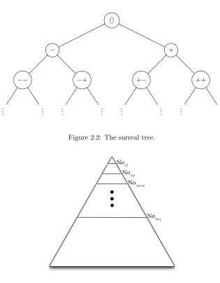
Given the previous definition it easy to see that No has a natural binary tree structure (see Fig.2.2). Note that each level of the tree corresponds to a set of surreal numbers with the same length. In particular we can define:

Definition 2.3.3. LetNobe the class of surreal numbers andα∈Onbe an ordinal. We define the following sets:

Noα={+,−}α i.e. the set of sequences of length exactlyα,

No≤α=

[

β≤α

Noβ i.e. the set of sequences of length less or equal to α,

No<α=

[

β<α

No≤β i.e. the set of sequences of length less than α.

Note that from this definition it is not hard to see that No≤α= No<α∪Noαand Noα= No≤α\No<α.

hi

−

−−

..

. ...

−+

..

. ...

+

+−

..

. ...

++

..

. ...

Figure 2.2: The surreal tree.

Figure 2.3: The subtrees of No.

Theorem 2.3.4 (Alling). Let κ0 be a regular cardinal. Then No<κ0 is a real closed field.

Proof. See [1, Theorem 6.22].

An extended study of these trees can be found in [11] and [1].

The following theorem will have a central role in the definition of operations over surreal numbers.

Theorem 2.3.5 (Gonshor, Simplicity Theorem). Let L and R be two sets of surreal numbers such that

L < R. Then there is a unique surrealz, denoted by [L|R], of minimal length such that L <{z}< R. We will call [L|R]a representation ofz.

Proof. See [14, Theorem 2.1].

Given two finite family of sets of surreal numbers S0. . . Sn and S00 . . . S0m, we will use the following

notation:

[S0, . . . , Sn|S00, . . . , S

0

m] = [

[

i≤n

Si|

[

i≤m

S0_i].

Each surreal number has many different representations, the following theorem gives us a canonical representation.

Theorem 2.3.6 (Gonshor). Let x ∈ No be a surreal number, L and R be two subsets of No defined as follows:

L={y|x < y∧y⊂x},

R={y|x > y∧y⊂x}.

Then[L|R] =x.

Proof. See [14, Theorem 2.8].

We will call the representation given by Theorem 2.3.6 thecanonical representation ofx. Note that the canonical representation just says that the elements of L are the proper initial segments y of xsuch that

x(|y|) = + and the elements ofRare the proper initial segments y ofxsuch thatx(|y|) =−. For example the canonical representation of +−+ is [(),(+−)|(+)], which means that +−+ is the shortest number between +−and +. As we will see, representations have an important role in developing surreal numbers theory. For this reason we will introduce some theorems which allow to manipulate and characterize these representations.

Theorem 2.3.7 (Gonshor). Let Land R be two sets of surreal numbers such that L < R. Then|[L|R]|is smaller or equal to the least ordinalαsuch that:

∀x∈L∪R.|x|< α.

Proof. Note that this follows trivially from the fact that [L|R] is defined to be de shortest surreal number strictly betweenL andR, then if it is of length bigger than α. Hence [L|R]αwould be shorter than [L|R] and still in betweenLand R.

Theorem 2.3.8 (Gonshor). Let x, y ∈ No be two surreal numbers and [Lx|Rx], [Ly|Ry] be respectively a

representation ofxandy. Thenx≤y iff{x}< Ry andLx<{y}.

Proof. We have Lx <{x} < Rx and Ly <{y} < Ry. Assumex≤ y then trivially {x} ≤ {y} < Ry and

Lx<{x} ≤ {y}. Assume{x}< Ry andLx<{y} andy < x. We haveLx<{y}<{x}< Rxhencexis an

initial segment ofy. MoreoverLy <{y}<{x}< Ry then y is an initial segment ofx. Hence x=y which

contradicts our assumption.

Finally we present three theorems from [14] which are very useful to find out when two different repre-sentation represent the same surreal number.

Definition 2.3.9(Cofinality). [L|R] is cofinalin [L0|R0] iff:

∀x0∈R0∃x∈R. x≤x0 ∧ ∀y0 ∈L0∃y∈L. y≥y0.

Moreover, given two representations[L|R]and[L0|R0]they are mutually cofinaliff[L|R]is cofinal in [L0|R0]

and[L0|R0] is cofinal in [L|R].

Note that this definition is totally consistent with the standard definition of cofinality (see Definition 2.1.2).

2.3.2

Operations Over

No

In this section we will define addition and multiplication over surreal numbers. First of all let us introduce some notation which will simplify the definition of the operations over surreal numbers. If S andS0 are a sets of surreal numbers,xis a surreal number and Op a binary operation over the surreal numbers, then we define

SOpx={sOpx|s∈S}, xOpS={xOps|s∈S}

and

SOpS0 ={xOpy|x∈S∧y∈S0}.

We begin the study of the surreal operations by defining the addition and its inverse.

Definition 2.3.12(Surreal Sum and Inverse). Let xandy be two surreal numbers and [Lx|Rx],[Ly|Ry]be

their canonical representations. Then we define the sumx+sy as follows:

x+sy= [Lx+sy, x+sLy|Rx+sy, x+sRy].

Moreover we define the inverseof x as the surreal number obtained by reverting all the signs. It is easy to see that that [−Rx| −Lx] where

−Rx={−xR|xR∈Rx}

and

−Lx={−xL|xL∈Lx},

is a canonical representation of −x.

The previous definition was given by induction over the maximal length of the addends. Note that we defined +s and−sonly for canonical representations. The following theorem tells us that the choice of the

representations we used does not matters.

Theorem 2.3.13. Let [Lx|Rx]and[Ly|Ry]be two representations respectively ofxandy. Then

x+sy= [Lx+sy, x+sLy|Rx+sy, x+sRy].

Proof. See [14, Theorem 3.2].

The intuition behind the definition of +s is thatx+sy can be thought to be the smallest number such

that the following inequalities hold:

Lx+y < x+y < Rx+y,

x+Ly< x+y < x+Ry.

Then the definition of x+sy is exactly reflecting this intuition, in factx+sy is defined to be the shortest

surreal number for which the previous inequalities hold. Let us consider some examples of sum.

Example 2.3.14. Consider the sequence+and its inverse−. Lethibe the empty sequence2_{. Then we have}

(+) = [hi|∅]and(−) = [∅|hi],

wherehiis the empty sequence. Then(+) +s(−) = [∅|∅] =hi. Therefore it is natural to define0 =hi. Now

denote (+)as1. Finally we have

1 + 1 = (+) +s(+) ={1 +s0,0 +s1|}.

Definition 2.3.15 (Surreal Product). Let x and y be two surreal numbers and [Lx|Rx], [Ly|Ry] be their

canonical representations. Then we define the productx·sy as follows:

x·sy= [Lx·sy+sx·sLy−Lx·sLy, Rx·sy+sx·sRy−Rx·sRy

|Lx·sy+sx·sRy−Lx·sRy, Rx·sy+sx·sLy−Rx·sLy].

Also in this case the definition is by induction over the maximal length of the factors, and as before the definition is uniform (the interested reader is referred to [14] Theorem 3.5). Let us illustrate how this definition works with an example.

Example 2.3.16. We have already defined0 =hi, 1 = + and2 = ++. Let us consider the multiplication

2·s1. First note that trivially:

0·s1 = 0·s1 = [∅|∅] = 0

and

0·s2 = 0·s2 = [∅|∅] = 0.

Moreover we have

1·s1 = [0·s1 +s1·s0−0·s0|∅].

Therefore

1·s2 = [0·s2 +s1·s1−0·s1|∅].

In conclusion1·s2 = [1|∅] = 2.

The last operation we introduce is the inverse of the product. While the previous definitions are quite intuitive the definition for the inverse of·sis more complicated. First of all one should convince himself that

the naive definition, namely

1

y = [0,

1

Ly

| 1

Ry

]

does not work. In particular this definition is such that 1_y ·sy6= 1 for somey∈No. To see this it is enough

to compute some left element of 1₃ ·s3 and check that it is bigger than 1. In particular we would have 1

3 = [0,1, 1

2|∅] and 3 = [0,1,2|∅]. But then 3 +s 1

3−s1 would be a left element of 1

3·s3, and by using the

definition of +s and−s we would have 3 +s 1₃−s1>1.

The main idea behind the definition of inverse of·s is that of setting the values in 1_y in such a way that

the left elements of 1

y·sy are smaller than 1. We define the inverse of·sby induction over the length ofy as

follows:

Definition 2.3.17 (Product Inverse). Let y ∈ Nobe a positive surreal number and let {Ly|Ry} be a

rep-resentation of y such that Ly, Ry > {0}3. By induction over the length of y assume that the inverse has

already been defined forLy andRy. We define the following sequences:

hi= 0,

hy0, . . . yni=xfor everyy0, . . . , yn∈Lx∪Rx\ {0},

where xis the solution of the equation(y−syn)·shy0, . . . yn−1i+yn·sx= 1. Note that a solution for this

equation exists by inductive hypothesis. Now we define:

1

y = [L1y|R

1

y],

where:

L1

y ={hy0, . . . , yni |n∈N the number of0≤i≤nsuch that yi∈Ly is even}

and

R1

y ={hy0, . . . , yni |n∈N the number of0≤i≤nsuch that yi∈Ly is odd}.

As for the previous definitions also the definition of product inverse is uniform.

A class field is a proper class C whose members satisfy the axioms of the theory of real closed fields4 (i.e., every axiom of the theory of real closed fields instantiated with members ofC can be proved). Given this definition, we can now mention an important result:

Theorem 2.3.18. The surreal numbers Noendowed with+sand·sform a class field.

Proof. See [14, Theorem 3.7].

Since in this thesis we will mostly be dealing with surreal operations, when no confusion arise we will drop the s from·sand +s.

2.3.3

Real Numbers and Ordinals

In this section we will show how to interpret real numbers and ordinal numbers within the class field of surreal numbers.

Before we show how real numbers are represented we consider the easier case of integers. We have already given some basic example showing how to represent 0, 1 and 2. Our intuition lead us to think that natural numbers are just finite sequences of pluses. Formally we have the following theorem:

Theorem 2.3.19 (Gonshor). For alln∈_N,(+)n _{is the positive integer nand(−)}n _{is its inverse.}

The dyadic rational numbers are those rational numbers of the form n

2m with n∈ Zand m ∈N. The

surreal numbers of finite length can be identified with the ring of dyadic rational numbers as shown by the following theorem:

Theorem 2.3.20 (Gonshor). Surreal numbers of finite length corresponds to dyadic numbers. Let d∈No

be a surreal number of finite length such thatnis the smallest such that∀i, j < n. d(i) =d(j)∧d(n)6=d(0). Define a sequence of dyadic numbers sas follows:

s(i) = +1 iffi < n∧i= +, s(i) =−1 iffi < n∧i=−, s(i) = + 1

2i−n+1 iffn≥i∧i= +,

s(i) =− 1

2i−n+1 iffn≥i∧i=−.

Thend=P|d|−1

i=0 s(i).

Proof. See [14, Theorem 4.2].

Intuitively the previous theorem says that a surreal numberdof finite length can be interpret as follows: take the longest prefixpofdin which there is no change in sign. Thend=s(0)|p|P|d|−1

i=0 s(|p|+i) 1 2i. For

example consider the sequenced= + +− −+, then we have thatd= 1 + 1−1 2−

1 4+

1 8 =

11 8.

Now we are ready to characterize the real numbers.

Definition 2.3.21 (Real Numbers). A surreal numberr is a real number iff either rhas a finite length or |r|=ω and for alli < ω existsj < ω such that i < j andr(i)6=r(j).

The previous definition says that a surreal number is a real number only if it is a dyadic or if it is of lengthωand not eventually constant.

0

−1

−2

.. .

−ω

.. .

.. .

.. .

−1 2

..

. ...

+1

1 2

..

. ...

+2

..

. ...

..

. +ω

.. .

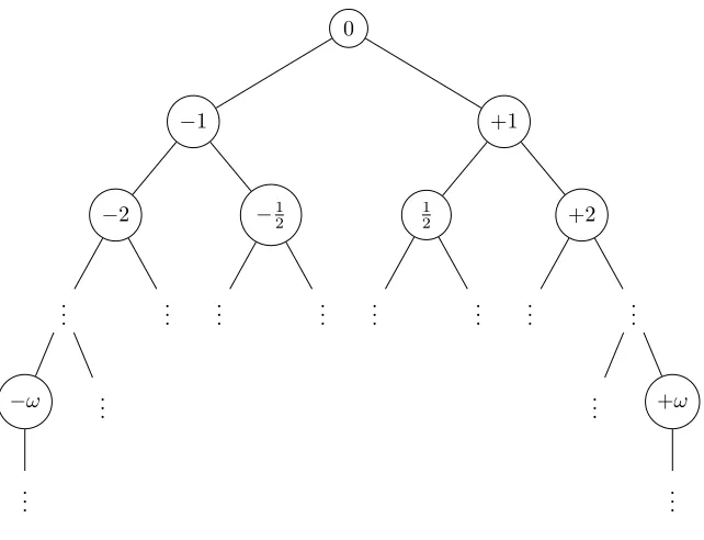
Figure 2.4: The surreal tree.

Finally will identify every ordinal αwith the constant sequence of pluses of length α. We will denote such a sequence by (+)α.

Note that this fits completely with the definition of positive integers we have just given. Moreover the order is trivially preserved, namelyα < β implies (+)α _<(+)β_{. Note that α+ 1 = [{β|β ≤α}|∅] and ifα}

is limit thenα= [{β|β < α}|∅]. Then from the order theoretic point of view we can identify ordinals and sequences of pluses.

Now if we look at the operations, the situation seems different. First of all we know that surreal operations are commutative while ordinal operations are not, for example ω+s1 = 1 +sω while ω+ 16=ω = 1 +ω.

In his introduction to surreal numbers Gonshor proved that the surreal operations over ordinal numbers correspond to theHessenberg (natural) operations.

2.3.4

Normal Form

In this section we will introduce a normal form for surreal numbers which is a generalization of Cantor’s normal form for ordinal numbers.

Definition 2.3.23 (Archimedean Equivalence Relation). Given two positive surreal numbers x and y we define the following equivalence relation:

x∼a y iff∃n∈Z. n·sy≥x ∧ n·sx≥y.

The equivalence classes induced by this relation are called orders of magnitude.

One interesting fact of the orders of magnitudes is that they have canonical representatives.

Theorem 2.3.24(Gonshor). Letxbe a positive surreal number. Then there is a uniquey of minimal length such that x∼ay.

These canonical elements can be parametrized using surreal numbers and the ω-map. Intuitively, the

ω-map is defined by lettingω0 be the shortest canonical element, namely 1, ω1 andω−1 be respectively ω

and 1

Definition 2.3.25 (ω-map). Let xbe a surreal number. We define:

ωx= [0, r·sωLx|s·sωRx],

wheres andrare positive real numbers,

ωLx _={ωxL _|x

L∈Lx}

and

ωRx _={ωxR_|x

R∈Rx}.

The fact that the ω-map is represented as an exponentiation is because it behaves as one would expect from the exponentiation operator.

Theorem 2.3.26 (Gonshor). Letx,y be two surreal numbers. We have: • ωx·sωy=ωx+sy.

• If xis an ordinal thenωx _{is the same as the usual ordinalω}x_.

• ωx_·

sω−x= 1.

In order to define the normal form of surreal numbers we need transfinite sums. Let αbe an ordinal, (xγ)β∈αbe a strictly decreasing sequence ofαsurreal numbers and (rβ)β∈αbe a sequence ofαnon-zero real

numbers. Then we define the sumP

β<αω xβ_·

srβ as follows:

X

β<γ+1

ωxβ_·

srβ=

X

β∈γ

ωxβ_·

srβ+sωxγ·srγ ifα=γ+ 1,

X

β<α

ωxβ_·

srβ = [L|R] ifαlimit,

whereLandR are defined as follows:

L={X

γ≤β

ωxγ_·

ssγ: [β < α]∧[∀γ < β. sγ =rγ]∧

[sβ=rb−twitht any positive real number ]},

R={X

γ≤β

ωxγ_·

ssγ : [β < α]∧[∀γ < β. sγ =rγ]∧

[sβ=rb+twitht any positive real number ]}.

Theorem 2.3.27(Conway, Normal Form Theorem). Every surreal number can be expressed uniquely in the formP

β∈αω xβ_·

srβ.

Proof. See [14, Theorem 5.6].

Note that the Cantor normal form is a special case of surreal numbers normal form.

2.4

Baire Space and Generalized Baire Space

In this section we will briefly recall some notion from basic descriptive set theory and generalized descriptive set theory. All the results in the first part of this section can be found in the first chapter of any introductory book of descriptive set theory such as [17].

Definition 2.4.1 (Baire Space). Let ωω _{be the set of sequences of natural numbers of lengthω. For every}

finite sequence of natural numbers w∈ω<ω _{we define the following set:}

[w] ={p∈ωω|w⊂p},

namely [w]is the set of infinite sequences that start with w. The set

Note thatωωis by definition second countable.

Lemma 2.4.2 (Folklore). Baire space is Hausdorff.

Proof. Letp, p0 ∈ωω _{such that p6=p}0 _{andnbe the smallest natural numbers such that p(n)6=p}0_{(n). Now}

[pn] and [p0n] are open sets. By the fact that p(n) 6=p0(n) we have that [pn]∩[p0n] = ∅. Moreover,

p∈[pn] andp0 ∈[p0n] as desired.

Baire space is easily proved to be totally disconnected.

Lemma 2.4.3 (Folklore). Baire space is totally disconnected.

Proof. We need to prove that for everyw∈ω<ω_{, the set [w] is closed. LetW be defined as follows:}

W ={w0∈ω<ω | ∃n∈ω. w(n)6=w0(n)}.

Thenωω_{\[w] =}S

W. Henceωω_{\[w] is open and [w] is closed as desired.}

Baire space is completely metrizable with the following metric5:

d(p, p0) =

(

0 ifp=p0_,

1

n+1 ifnis the least such thatp(n)6=p

0_(n).

One important property of Baire space is that it is homeomorphic to the product topologyQ

α∈ωωwhere

ω is endowed with the discrete topology.

Now we will recall some basic definitions and properties of generalized Baire spaces. In particular we will generalize the notions we have just seen to the cardinalκwe have fixed at the beginning of this chapter. All the notions that we will present in the rest of this section can be found in [13].

Definition 2.4.4(Generalized Baire Space). Letκκ _{be the set of sequences of ordinals inκof lengthκ. For}

every sequencew∈κ<κ _{of elements ofκof length less than κ, we define the following set:}

[w] ={p∈κκ|w⊂p}.

Then the set

B={[w]|w∈κ<κ}

is a base. We will call the setκκ equipped with the topology induced byB generalized Baire space.

Note that the assumption κ<κ =κ, is necessary in order for generalized Baire space to have a base of cardinality κ and then a dense subset of cardinality κ. As we will see this will be crucial for generalize computable analysis. By using the same proofs of the classical case it is not hard to see that generalized Baire spaceκκ _{is Hausdorff and totally disconnected.}

We want to end this section by mentioning to important differences between the Baire space ωω _{and its}

uncountable generalizations.

Theorem 2.4.5. Generalized Baire space is not metrizable.

Proof. First of all recall from topology that if a space X is metrizable, then for every x∈ X, there is a countable setNxof open sets such that for every open setU containingxthere isV ∈N such thatV ⊂U.

Assume that κκ is metrizable. Letpbe an element ofκκ. For every element of U ∈Np take a basic open

set [wU] which containsxand such that [wU]⊂O. Since there are only countably many of these open sets

andκis a regular cardinal bigger thanω, there isw∈κκ_{such that for everyU ∈N}

p, we havewU ⊂w. But

then x∈[w] and for every U ∈Np we have U 6⊆[w]. This contradicts our hypothesis, therefore κκ is not

measurable.

Hence there is no notion of a metric which inducesκκ_{. In particular this means that all the notions that}

depend on the metrizability ofκκ_{(e.g. the Borel hierarchy) have to be either reformulated in a non-metric}

way or cannot be generalized toκκ.

Finally, generalized Baire space is not homeomorphic to the product topologyQ

α∈κκ, whereκis endowed

with the discrete topology (see [13]).

5_{Note that, even though this is not the standard definition of the metric overω}ω_{, it is completely equivalent to the classical}

one from the topological point of view. As we will see in Chapter 3 this definition will generalize in a straightforward way to

κκ_{by using}

2.5

Computable Analysis

In this section we will present some basic notion from classical computable analysis and we will set up some conventions that we will use all over this thesis. A complete introduction to computable analysis can be found in [28] and a topological introduction to the more general theory of represented spaces can be found in [23]. Where it is possible, we will use the same notation as in [28].

2.5.1

Effective Topologies and Representations

The intuition behind computable analysis is that of generalizing computability theory to uncountable sets. In order to do this, the idea is that of study computational and topological properties of the Baire spaceωω

(or the Cantor space 2ω_{) and then, transfer these results to any uncountable set by means of coding. These}

codings have a central role in computable analysis, therefore we recall their definition.

Definition 2.5.1 (Representation). Let M be a countable set. Then a notation over M is a surjective partial function from the set of finite sequences of natural numbersω<ω toM. IfM has cardinality2ℵ0 then a surjective partial function with domain the Baire space ωω and codomain M is called a representation of

M. Ifδ is a representation overM, we will call (M, δ)a represented space.

Definition 2.5.2(Reductions). Letδ:⊆ωω_{→M andδ}0_:⊆ωω_{→M be two representations ofM. Then we}

will say thatδcontinuously reduces toδ0, in symbols δ≤tδ0 iff there is a continuous functionh:⊆ωω→ωω

such that for everyx∈dom(f),δ(x) =δ0(h(x)).

If δ≤tδ0 andδ0≤tδ we will say thatδ andδ0 are continuously equivalent and we will write δ≡tδ0.

Continuous reductions are a very useful tool, and as we will see they can be used to see how representations behave with respect to the topological properties of the space they represent.

Note that usually in computable analysis to any continuous notion correspond a computable notion, for example we could consider computable reductions instead of continuous reductions. The reason why we will only present the topological aspects of computable analysis is that it is still not clear how to define a notion of computability overκκ_.

Effective topological spaces form a particularly well-behaved subclass of spaces. They induce naturally a standard representation which turns out to be a quotient map with respect to the topology of the space they represent.

Definition 2.5.3 (Effective Topological Space and Standard Representation). Let M be a set, σ be a countable family of subsets of M such that

x=y iff{A∈σ|x∈A}={A∈σ|y∈A}

andν :⊆ω<ω_{→σ be a naming onσ. Then S= (M, σ, ν)is an effective topological space. We will call τ} s

the topology generated by takingσas a subbase andδS :⊆ωω→M the standard representationofS defined

as follows:

δS(p) =xiff{A∈σ|x∈A}={ν(w)∈ι(w)/ p} ∀p∈ωω.

Intuitively, given an effective topological space, we can think atσas a list of properties that can distinguish elements ofM and atν as the way we can access them. From this point of view,p∈ωω_{is a code forx∈M}

according to the standard representation if and only ifpcodes the list ofall the properties which characterize

x.

As we have already said, effective topological spaces are a particularly well-behaved subclass of represented spaces. This is due to the fact that in this specific case the topological space τS and the final topology

induced by δS are the same. This implies that some important properties ofτS transfer to Baire space and

vice versa. The following lemma shows how strong is the connection between an effective topological space and its induced topology.

Lemma 2.5.4. LetS= (M, σ, ν)be an effective topological space,δS its standard representation andτS the

• δS is continuous and open w.r.tτS.

Proof. See [28, Lemma 3.2.5].

This lemma is important to establish a connection between Baire space and the topology τS. Let us

illustrate how effective topological spaces work with an example.

Example 2.5.5. Let us consider the set of real number _R. We already know that, in order to do analysis over _R we will want to use the interval topology τ_R over _R. Then it is natural look for a representation which induces this topology. We can use the well known fact that the set of open intervals with endpoints in Qis a base for τR and the fact that Qis countable to define an effective topological space whose induced topology isτ_R. Letν_Q:⊆ω<ω _→

Qbe any notation overQ(it is not hard to explicitly define one). Moreover

let _p·,·_q : ω<ω_×ω<ω _→ω<ω _{be any pairing function. Then we can define a notation for the set of open}

intervals with rational endpoints Cbas follows:

I(_pi, j_q) =B(ν_Q(i), ν_Q(j)),

where B(q, q0)is the open ball with center q and radius q0. Define S= (R,Cb,I). Now, since Cbis a base

for the interval topology over _R, then τS is the interval topology over R. Moreover, for what we have just

shown, δS is continuous and open with respect to this topology.

Lemma 2.5.6. Let M be a set,δ0 :⊆ωω →M and δ1 :⊆ωω→M be two representations. Moreover, let

τ0 andτ1 be respectively the final topology induced byδ0 and δ1. Thenδ0≤tδ1 impliesτ1⊆τ0. Moreover,

givenδ₀0 :⊆ωω_{→M andδ}0

1:⊆ωω→M be other two representations ofM, such thatδ00≤tδ0 andδ10 ≤tδ1.

Then every(δ0, δ1)-continuous function is (δ0, δ1)-continuous.

Proof. Let f :⊆ ωω _{→ ω}ω _{be a continuous reduction of δ}

0 to δ1 and O ∈ τ1. By definition δ1−1(O) is

open in dom(δ1). Moreover, since f is continuous, f−1δ1−1(O) is open in dom(f)∩f−1(dom(δ1)). Then

f−1_δ−1

1 (O) is open indom(f)∩f−1(dom(δ1))∩dom(δ0). Now, sincef is a reduction ofδ0 to δ1, we have

dom(f)∩f−1(dom(δ1))∩dom(δ0) = dom(δ0) andδ−01(O). HenceO∈τ0 as desired.

Now let f be a (δ0₀, δ0₁)-continuous function. Consider a continuous reduction h0 of δ0 to δ00 and a

continuous reduction h1 of δ1 to δ10. Let F be a continuous realizer of f. Then h1◦F ◦h0 is a (δ0, δ1

)-continuous realizer off.

Since continuous reductions preserve many topological properties we are interested in, it is natural to use them to characterize a well-behaved class of representations.

Definition 2.5.7 (Admissible Representation). Let (M, τ) be a topological space. Then a representation

δ:⊆ωω _{→M is κ-admissible w.r.t. τ iffδ is continuous and every continuous function ϕ:⊆ω}ω_{→M is}

continuously reducible toδ.

Note that, as shown in [24], a representationδof a topological space (M, τ) is admissible iff it is contin-uously equivalent to a standard representation of an effective topological spaceS= (M, σ, ν) withτS =τ.

In classical computability theory representations are used to transfer computability form the natural numbers to any countable space. The same approach is taken in computable analysis, where representations allow to transfer notions of continuity and computability from Baire space to any space of cardinality at most 2ℵ0. Realizers have a central role in this construction.

Definition 2.5.8. Let F :⊆ M1 → M0 be a function over two represented spaces (M1, δ1) and (M0, δ0).

Thenf :⊆ωω→ωω is a realization ofF iff for everyx∈dom(δ1),F(δ1(x)) =δ0(f(x)). Iff is continuous

we will say thatF has a continuous realizer w.r.t. δ1 andδ0 or for short that F is(δ1, δ0)-continuous.

Theorem 2.5.9 (Main Theorem of Computable analysis). For i = 0, . . . , n let δi :⊆ ωω → Mi be an

admissible representation w.r.t. the topologyτi. Then for any function f :⊆M1×. . .×Mn →M0 we have:

f is continuous ⇔f is(δ1, . . . , δn, δ0)-continuous.

Proof. See [28, Lemma 3.2.11].

In particular the main theorem of computable analysis tells us that admissible representations respect continuous functions over the topological spaces they induce.

Example 2.5.10. Let us continue our example on R. LetS = (R,Cb,I) be the effective topological space

defined in the Example 2.5.5. We know that τS is the interval topology overR. now, since is a well-known

fact that +and× are continuous over the interval topology, the main theorem of computable analysis tells us that+and×are continuously represented over Baire space.

The main theorem of computable analysis is important in computable analysis and in all those cases in which we already have a standard topology over the space we want to work with. In these cases, indeed, effective topological spaces and admissible representations give us a strict correspondence between continuous functions between represented spaces endowed with their intended topologies and the continuous functions over Baire space. This fact will turn out to be also important for representing the set of continuous functions between representable spaces.

Note that, in some cases a completely different approach is possible. In particular if we do not have a preferred candidate for the topology we want to use over the represented space we are working with, then we can just fix any representation and work with the final topology induced by this representation. In this case we would still have the main theorem of computable analysis w.r.t. the final topology and then a natural way to represent the space of continuous functions on our space.

2.5.2

Subspaces, Products and Continuous Functions

In this section we will briefly recall some constructions over representations.

First of all we consider subspaces of represented spaces. Note that, since restriction of surjective functions are still surjective, for every represented spaces (M, δM) and subsetM0ofM the restrictionδMM0ofδM to

M0 is still a representation of M0. Moreover, it turns out that the restriction of admissible representations

is still admissible.

The second construction that we take into consideration is product. Before we can give the definition of product of representations we need to define some tupling functions. Fix a bijection_p·,·_q:ω×ω →ω. Then we define:

Definition 2.5.11 (Tupling Functions). Let a1, a2. . . , ai with i < ω be a sequence of element of ω. We

define a wrappingfunctionι as follows:

ι(a1, a2, . . . , ai) = 110a10a20. . .0ai011.

Moreover given x1, x2, . . .in ω<ω andp1, p2. . . , inωω, we define:

px1, p1q=pp1, x1q=ι(x1)p1∈ωω,

px1, . . . , xiq=ι(x1). . . ι(xi)withi < ω, px1, x2. . .q=ι(x1)ι(x2). . . ,

pp1, . . . , piq=p1(0). . . pi(0)p1(1). . . pi(1). . . withi < ω, pp1, p2. . .qpi, jq=pi(j)for alli, j∈ω.

Definition 2.5.12. For every i∈ω, let (Mi, δi) be a representation. Then we define the productNi∈ωδi

as follows:

(O

i∈ω

δi)ppi. . .qi∈ω= (δi(pi))i∈ω.

For everyn∈ω, we define the product N

i∈nδi as follows:

(O

i∈n

δi)pp0, . . . , pn−1q= (δ0(p0), . . . , δn−1(pn−1)).

Also in this case we have that the product of effective topological spaces is an effective topological space whose standard representation is the product representation and the induced topology is the product topology.

We will now consider the space of continuous functions between represented spaces. As we said the main theorem of computable analysis will turn out to be important in this context. Given two representable spaces (M0, δ0) and (M1, δ1) we want to represent the space of functions between M1 and M0 with a continuous

realizer (note that this is the same as the space of continuous functions w.r.t the final topologies induced by

δ1and δ2). We will denote the set of continuous functions from M1 toM0 with C(M1, M0), sometimes the

codomain is clear from the context in those cases we will write C(M1).

Definition 2.5.13. Let(M0, δ0)and(M1, δ1)be two represented spaces andC(δ1, δ0)be the space of(δ1, δ0)

-continuous functions. Then we define a representation[δ1→δ0] ofC(δ1, δ0) as follows:

[δ1→δ0](hn, pi) =f ifff is the function computed by the n-th Turing Machine with oraclep,

for everyhn, pi ∈ωω_.

Definition 2.5.13 strongly depends on Turing machines and on the notion of computability over ω. As we will see, since we lack these notions for the generalized Baire spaceκκ_{, we will have to give a definition}

based on the topological properties rather than on computational notions.

2.5.3

The Weihrauch Hierarchy

As we said in the introduction,our main aim is that of study the complexity of theorems from classical analysis in the context of the generalized Baire spaceκκ_{. In the classical case, Weihrauch reductions are the}

main tools to compare and classify theorems. For an introduction to the theory of Weihrauch reductions see [5].

First, since we will be using multi-valued functions to represent theorems form analysis, we need to extend the definition of realizer:

Definition 2.5.14 (Multi-Valued Functions Realizers). Let F :⊆ M1 ⇒ M0 be a multi-valued function

between the represented spaces(M1, δM1)and(M0, δM0). Then,f :⊆ω

ω_→ωω_{is a realizer ofF iff for every}

x∈dom(dom(F◦δM1)we have

δM0(f(x))∈F(δM1(x)).

If F has a continuous realizer we will say that it is(δM1, δM0)-continuous.

Weihrauch degrees can be used for classifying the complexity of functions over Baire space. This, to-gether with the theory of representable spaces, makes them a natural tool for classifying functions between represented spaces.

Definition 2.5.15 (Weihrauch Reductions). Let F :⊆M1 ⇒M0 and G:⊆N1 ⇒N0 be two multi-valued

functions between represented spaces. We will say thatF is Weihrauch reducible toG, in symbols F ≤wG

iff there are two continuous functions H :⊆ ωω _{→ ω}ω _{and K :⊆ ω}ω _{→ ω}ω _{such that for every realizer}

g:⊆ωω_→ωω _{of Gthere is a realizer f :⊆ω}ω_→ωω _{of F such that}

where ID : ωω → ωω is the identity function. Moreover, if H and G are such that for every realizer

g:⊆ωω→ωω of Gthere is a realizer f :⊆ωω→ωω of F such that

f =H◦g◦K,

then we will say that F is strongly Weihrauch reducibletoG, in symbolsF ≤s,wG.

By using Weihrauch reductions one can study the complexity of functions between represented spaces. A particularly significant case of the use of Weihrauch reductions is that of computable analysis. Many theorems from analysis are in fact of the form:

∀x∈X∃y∈Y.P(x, y),

whereP is quantifier free. In this case a theorem can be seen as a multi-valued function betweenX andY

which given an element ofX returns an element ofY such thatP(x, y) holds. This fact makes Weihrauch reductions a natural tool for comparing theorem from real analysis. Let us illustrate this fact with an example:

Example 2.5.16. Let us consider the Intermediate Value Theorem (IVT). It can be stated as follows: Let f : [0,1]→Rbe a continuous function such that f(0)·f(1)<0. Then there isr ∈[0,1]such that

f(r) = 0. LetC0[0,1] be the set of continuous functions from[0,1]to_R. Since we have already seen that_R is representable and[0,1]⊂_R, the restriction ofδ_R is an admissible representation ofC0[0,1]. By the Main Theorem of Computable Analysis we have that C0[0,1]has a representation induced by the representation of continuous functions over Baire space. Then the setC[0,1]of continuous functions such thatf(0)·f(1)<0

is also represented. Then it is not hard to see that the IVT can formalized as follows:

IV T : C[0,1]→[0,1],IV T(f) =r⇔f(r) = 0.