On Evolution of Compositionality
MSc Thesis
(Afstudeerscriptie)
written by
Sanne Brinkhorst
(born September 11, 1988 in Rotterdam, the Netherlands)
under the supervision of Dr. Michael Franke, and submitted to the Board of Examiners in partial fulfillment of the requirements for the degree of
MSc in Logic
at theUniversiteit van Amsterdam.
Date of the public defense: Members of the Thesis Committee:
Abstract
Contents
1 Introduction 2
2 Background 4
2.1 Signalling games . . . 4
2.2 Animal signalling . . . 5
2.3 Evolutionary dynamics . . . 6
2.4 Evolutionary dynamics in Lewis signalling games . . . 8
2.5 Reinforcement learning . . . 10
2.6 Variations on the basic urn learning model . . . 10
3 Automaton models 13 3.1 Introduction . . . 13
3.2 Technical framework . . . 14
3.3 Methods . . . 20
3.4 Results . . . 21
4 Neural Networks 26 4.1 Introduction . . . 26
4.2 Technical framework for simple Lewis game . . . 27
4.3 Technical framework for Lewis game with complex states . . . . 30
4.4 Methods . . . 30
4.5 Results . . . 32
5 Conclusions and further work 36 5.1 Conclusions . . . 36
Chapter 1
Introduction
How did the first word get its meaning? Suppose that that first word was the imitation of a sound and the answer is simple: it referred to what it sounded like. But most words we use do not sound like what they refer to, and not all objects we want to refer to have a sound we can imitate. Human language is a very advanced system: we can discuss virtually anything. Objects do not have to be around or even have to exist to refer to them. We can discuss feelings and fiction: things that are not visible. There is a long journey from the first intentionally produced noise to the language we use today. This thesis is about the first steps: how to combine different elements of a message and transfer meaning.
I will model communication as agents playing signalling games. In these games, introduced by David Lewis [7] (and therefore also called Lewis games), two agents have to coordinate an action by using messages. If the agents suc-ceed, they will receive a reward, if they fail they receive nothing. This theoretical framework has been used extensively to investigate the emergence communica-tive systems[14]. Most learning models use holistic messages: the entire sound or symbol is treated as a single message.
Two models of combinatorial message use will be presented. The combina-torial messages consist of individual parts that contribute to the meaning of the whole. The first model is an extension of reinforcement learning models that have been used successfully for information transfer with holistic messages. The second is based on artificial neural networks, models that are used in machine learning for pattern recognition.
Chapter 2
Background
2.1
Signalling games
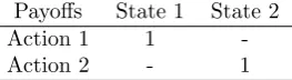
In his book Convention[7], David Lewis introduces signalling games. These games have two players: a sender and a receiver. The sender has some infor-mation about the world. The receiver needs to know this inforinfor-mation to choose the best action in the current state of the world, but has no direct access to it. If the receiver chooses the appropriate action, both agents will receive a reward, so it is in the senders interest to aid the receiver. In table 2.1 an example of the payoffs for such a game can be seen. The agents both receive exactly the same payoff, so there is no incentive for the sender to deceive the receiver and the receiver has no reason to distrust the sender. The problem is the following: the sender and receiver have no language to communicate. The sender has a set of signals he can use to convey information to the receiver. But these signals have no predefined meaning, so the receiver will not immediately know which state is indicated by which signal. By developing a convention the agents can learn to communicate with the signals.
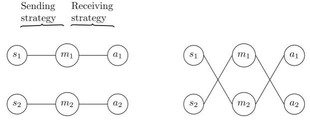
What exactly the convention is, is arbitrary. If there are two signals, it does not matter which one the sender uses to indicate state 1, as long as the agents use the same convention. In figure 2.1 two possible strategies for a situation with two states, two messages and two actions are shown. On the left is the strategy where the agent always sends message 1 when he observes state 1. When the agent receives a message, he will always choose action 1 if he hears message 1. The other message is exclusively used for the second state. On the right another strategy is shown, where the messages are used in exactly the opposite situation. Neither of the strategies is better: in both cases the agents will receive the payoff because they successfully communicate about the state.
Payoffs State 1 State 2
Action 1 1
[image:6.595.232.364.637.673.2]-Action 2 - 1
s1
s2
m1
m2
a1
a2
Sending strategy
Receiving strategy
s1
s2
m1
m2
a1
[image:7.595.142.453.127.251.2]a2
Figure 2.1: Strategies for a 2-state game
All strategies that result in maximum payoff are called signalling systems.
2.2
Animal signalling
When one compares the signalling game with the rich and complex language humans use, it might seem an oversimplification. But animal communication follows this pattern quite often, for example in alarm calls. When one animal perceives a potential harmful situation, for example a rival group or a predator, it sounds an alarm call to alert the other animals in the group. These alarm calls are specific for the type of danger, because each danger requires a different action. Fight or flight is not the only decision: where to flee or how to fight depends on the situation.
For each predator, a different tactic is most suitable. Campbell’s monkeys (Cercopithecus c. campbelli) have several enemies: gaboon vipers, leopards and crowned eagles [8]. If an leopard is encountered, a common tactic for male and female Campbell’s monkeys is to climb in a tree and stay there for a while. This way the monkeys are out of reach for the leopard. Climbing high in a tree is not a good hiding tactic for aerial predators. If a crowned eagle is spotted, the female monkeys, who are smaller than the males, will go down in the tree or hide in the foliage. The males are approximately the same size as the crowned eagles and will go towards the eagle and attack it. Gaboon vipers are venomous and all monkeys avoid it by climbing in the trees. For these different enemies, Campbell’s monkeys have different types of alarm calls [9].
Campbell’s monkeys use very simple composition in their alarm calls. If some danger is in the area but no imminent treat, male Campbell’s monkeys will use a specific boom-like sound before the normal alarm call [17]. This communication is not only between animals of the same species: Diana monkeys live in the same area and will listen to the alarm calls. They will respond to normal alarm calls but in cases where the prefix is used they show little response.
There are also limited examples of more complicated communication in ani-mals, though it was not in a natural setting. In various experiments researchers tried to teach apes to communicate with symbols. Two young pygmy chim-panzees learned to communicate with symbols and gestures without formal training, by observing the training or use by other apes[12]. The eldest ape started to use new combinations of symbols and gestures, for example to re-quest that two caretakers would play chase together. All other apes only used verbs when they were one of the agents.
Monkeys are also capable of learning from input when their actions do not necessarily result in a reward. Yang and Shadlen [16] performed an experiment where rhesus monkeys had to make a choice between two targets. One of the targets would result in a reward. The monkeys would be presented four shapes out of a set of 10 possibilities. Each of these shapes corresponded to a weight which influenced the probability of the payoff. The monkeys would learn to choose the target that corresponds to the weights. If the evidence for the targets was neutral, they would select each target with chance 0.5. Because there are 104 combinations of shapes, it is not likely that the monkeys learned each
specific combination but that they combined the information of the targets. This experiments has two results that are important for signalling games: rhesus monkeys can learn a task when the options do not have a fixed payoff and can combine information of individual signals.
2.3
Evolutionary dynamics
To analyse the emergence of communicative behaviour, we model communica-tion as a game theoretic problem. We do not only look at the behaviour of the individual agents, but also how this behaviour develops in a population. In a population consisting of agents, all agents play the same game but with possible different strategies. Players are paired randomly and have no information about the strategy of their opponent.
2.3.1
Evolutionary stable strategies
An evolutionary stable strategy (ESS) [15], [14, ch. 4] is a strategy such that in a population of agents using this strategy, a small group of agents with a different strategy will not have higher payoffs. The agents of the smaller group are called mutants. A strategy S is evolutionary stable if all mutants do worse when playing against arbitrary players in the population.This is the case if i) payoff for S against S is higher than M against S orii) S and M do equally well when playing against S, but S against S results in a higher payoff than S against M.
Consider the game stag hunt (figure 2.2, left). In this game, players can cooperate for a big reward or work alone (defect) for a smaller reward. The highest payoff is when both players cooperate. But if a player cooperates and the opponent does not, the cooperator is left with nothing and would have been better off working alone too.
Stag hunt Cooperate Defect Cooperate 3 3 1 0 Defect 0 1 1 1 Prisoner’s dilemma Cooperate Defect Cooperate 3 3 4 0 Defect 0 4 1 1
Figure 2.2: Payoff matrices for stag hunt and prisoner’s dilemma
is 3p.1 The defectors always receive payoff 1 and will have a lower payoff ifpis close to 1.
On the other hand, if most players defect,pis very low and 3p <1 and a small group of cooperators will receive a lower payoff than the main population. An example of a strategy that is not evolutionary stable is the cooperate strategy in prisoner’s dilemma (figure 2.2, right). If everybody in the population cooperates, everybody receives payoff 3. But if a small group of defectors enters the population, they will perform better. If they encounter a cooperator they receive payoff 4 instead of 3 and if they encounter a fellow defector they receive 1 instead of 0. It is clear that defecting is an evolutionary stable strategy, because cooperation will never perform better.
2.3.2
Replicator dynamics
In evolution, three aspects are important: variation, reproduction and inheri-tance. The concept of evolutionary stability provides some insight in the dif-ferent strategies, which can be seen as variation in the population. For repro-duction and inheritance we will look at the replicator dynamics. This assumes that successful individuals reproduce more and that their offspring will inherit properties[14]. To model this, assume a population with agents of different types. At timet, the expected payoff for each typeSis calculated from the pro-portionsxt(S) of the types. This expected payoff is the fitness of the type. The number of offspring each individual gets depends on the fitness. The offspring are exact copies of the agent, there is no combination of strategies. For the new generation the proportion is calculated by comparing the fitness of the type to the average fitness:
xt+1(S) =xt(S)∗(Fitness(S)/Average fitness)
Types with a higher than average fitness will make up a larger proportion of the population for the next generation, while types with lower than average fitness will have a smaller new generation.
The proportions of a population with two types can be represented on a line. On one end, it represents a population with only type 1 agents, on the other end only type 2 agents. The points in between represent a mixed population.
In the case of stag hunt, we have seen that in populations with mainly coop-erators the coopcoop-erators have higher fitness and there will be more coopcoop-erators in the next generation. If there are mostly defectors, the defectors have higher fitness and the proportion of defectors will grow.
1A cooperator has probabilitypto encounter a cooperator and receive payoff 3 and
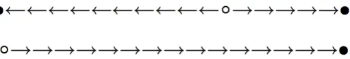
Figure 2.3: Population dynamics for stag hunt (top) and pris-oner’s dilemma (bottom). On the left of the line is the popula-tion with only cooperators, on the right only defectors. Figure from [14]
For the game stag hunt, there is a situation in which the proportions stay exactly the same: if 1/3 of the agents cooperates, both types have the same
expected payoff (1). If there are more cooperators, the proportion of cooperators will grow each round until there are almost no defectors left. If there are more defectors, this proportion will keep growing until everybody defects.2
In figure 2.3 the replicator dynamics of stag hunt are shown. On the left of the line the population with only cooperators is represented, on the right is the population of all defectors. The open point represents the 1/3cooperators, 2/3
defectors equilibrium. If the population is not exactly at the point of equilibrium it will move towards one of the ends.
Below the stag hunt is the situation for prisoner’s dilemma. The open point on the left represents a population with only cooperators. If there are no defec-tors, they cannot reproduce either. But if there is a tiny fraction of defecdefec-tors, this fraction will grow over the rounds until there are only defectors (on the right).
The black points are evolutionary stable strategies. The system will move towards these points. The white (open) points are not evolutionary stable and a small change in the population will cause the system to move away from this point.
2.4
Evolutionary dynamics in Lewis signalling
games
In figure 2.1 two possible strategies were shown for a 2×2×2 signalling game. But these are not all possibilities, these are only the signalling system: strategies that result in an optimal payoff if both agents use the same strategy.
An example of a strategy that is not optimal is a pooling strategy, which can be seen in figure 2.4 (left). The sender will always send the same message, independent of the state. The receiver always selects the same action, without listening to the message. Both cases result in expected payoff 0.5 for equiprob-able states. If another agent with a normally successful signalling strategy
2If we just look at proportions the agents of the other type will not always completely
s1 s2 m1 m2 a1 a2 s1 s2 m1 m2 a1 a2
Figure 2.4: Pooling strategy for a 2 state game (left) and an invading strategy (right)
s1 s2 s3 m1 m2 m3 a1 a2 a3 x
1−x
y
1−y
s1 s2 s3 m1 m2 m3 a1 a2 a3
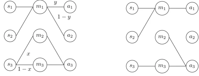
Figure 2.5: Mixed strategy (left) and a pure strategy (right) for a three state game. The mixed strategy is evolutionary stable for most values ofxandy, while the pure strategy can be invaded by signalling systems.
(displayed on the right) plays with pooling agents, the payoff will still be half: if the pooling agent sends a message it has no information and if the pooling agent receives the message he will not use the information. But for two states, these pooling strategies are not evolutionary stable. The invading, “smarter” agents will not do better against the general population, but will do better when playing each other. The non-pooling strategies are evolutionary stable.
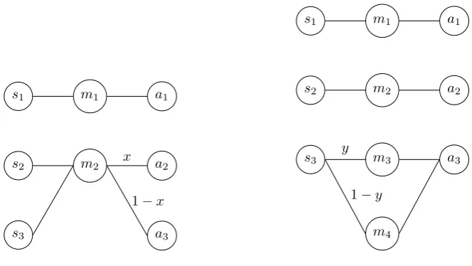
Thus far, the strategies discussed are pure strategies: the agents always select the same option in the same situation. There are, however, also mixed strategies: agents choose their actions based on a probability. In figure 2.5 on the left an example can be seen for a three state game. This example is immediately a problematic one: this strategy is suboptimal, but it is evolutionary stable for most values of x and y. The expected payoff is 2/3 for this strategy, but it is
not possible for a pure strategy to do better when playing against this mixed strategy.
[image:11.595.128.463.259.387.2]2.5
Reinforcement learning
Evolutionary dynamics tells us why some strategies will survive and thrive, while others will die out. This does not explain how these strategies emerged in the first place. At the level of individual agents, strategies can emerge by reinforcement learning. In reinforcement learning, actions that had good results in the past will be more likely to be selected again.
There are various models of reinforcement learning. One model is Roth-Erev reinforcement [10], where agents learn from their previous actions. The agent start by selecting actions randomly and keeps track of the rewards. The prob-ability if selecting an action again is proportional to the accumulated rewards. In this thesis Roth-Erev reinforcement will be used.
This process is also called urn learning, because it can be visualised as draw-ing balls from an urn. In the case of a signalldraw-ing game, the sender has an urn for each possible state. In each urn are balls that represent the messages. The sender perceives the state and draws a ball from the corresponding urn. If the receiver chooses the correct action, both receive payoff. The sender puts the message ball back in the urn, but adds more balls of the same type. The number of balls is proportional to the payoff. If no payoff was received, only the original ball is put back and the urn stays the same. When repeating this process, there will be more balls corresponding to the successful messages in the urn, making it more likely to draw these balls. The receiver has an urn for each message and these urns contain action balls. When hearing a message, the receiver consults the appropriate urn and performs the action corresponding to the ball that was drawn. Updating the receiver follows the same procedure as the sender.
Unless otherwise specified, the urns start with 1 ball of each type and the payoff for successful communication is also 1. Other proportions can be used as well, including negative payoff where balls are removed [2].
For 2×2×2 games with equiprobable states Roth-Erev reinforcement is very successful and will always converge to a signalling system[1]. If the states have unequal probabilities, this result no longer holds. The agents will not always develop a signalling strategy with meaningful messages and simply select the action that corresponds to the most likely state. For probabilities that are not far apart (0.6 for one state, 0.4 for the other) this happens not very often, but in more extreme inequalities it is very common.
Reinforcement learning is not always successful for games with more states. For a 3×3×3 game, pooling occurs in roughly 10% of the cases. This is even worse for larger games, for 8 states over half of the runs end in a pooling equilibrium.
2.6
Variations on the basic urn learning model
The games presented so far had exactly as many messages as states. If there are less messages than states, the agents cannot communicate perfectly. In a game with 3 equiprobable states and two messages the maximum expected payoff is
2/3. An example of such a strategy is shown in figure 2.6. Experiments show
s1
s2
s3
m1
m2
a1
a2
a3
x
1−x
s1
s2
s3
m1
m2
m3
m4
a1
a2
a3
y
[image:13.595.132.464.123.310.2]1−y
Figure 2.6: Signalling with too few (left) and extra (right) mes-sages
approached the best possible rate[2].
If there is a surplus of messages, agents can communicate perfectly. The extra messages may be unused, or be used as synonyms (figure 2.6). The success of games with extra messages is higher than of games with exactly enough messages [2]. Therefore it is relevant to look at models that are able to generate more messages.
2.6.1
Skyrm’s message innovation
The sender has urns for each state and starts with balls for each message and a magic ball. If the sender draws a message ball, the play is as usual. When the magic ball is drawn, a new message is invented and sent to the receiver. The receiver will choose a random action.
If this new message results in payoff, the new message is kept. All state urns get a ball for the new message and the actual state will get reinforced as well. The receiver will add a new urn for this message and reinforce it with the successful action. The magic ball is replaced in the state urn.
If the new message is not successful, only the magic ball is replaced and no other balls are added to the sender urns. When the magic ball is drawn again, the same message may be used again but treated as a new message.
Simulations show that if the sender starts without messages and only a magic ball, a signalling system will develop. After 100000 plays between 5 and 25 messages were invented. Most of the plays used a smaller subset of the messages and other messages were rarely used. The set of messages that are frequently used may be larger than the set of states, synonyms will occur.
2.6.2
Barrett-Skyrms multiple sender model
s1
s2
s3
s4
m1
m2
a1|a3
a2|a4
s1
s2
s3
s4
m1
m2
a1|a2
[image:14.595.134.492.124.294.2]a3|a4
Figure 2.7: A strategy for two senders to convey information about four states with only two messages. The receiver will combine the information of the two senders and have perfect information
the variation in sound production and can only produce a limited set of signals. Skyrms [14] introduced a model with two senders. Each sender has only two messages and cannot communicate all information about four states. By pooling two states to one message the sender can provide some information, increasing the expected payoff to 0.5. That is only if the senders use the same pooling strategy: if they pool their messages differently, sender 1 may indicate that s1 or s3 is the case, while sender 2 can indicate that s1 or s2 is the case.
When the receiver combines this information he will know thats1is the actual
state.
The receiver knows which message is sent by which sender, resulting in four unique combinations. Effectively the receiver learns to interpret an ordered pair of messages. The role of the two senders can be performed by a single sender producing a signal twice.
Chapter 3
Automaton models
3.1
Introduction
In this chapter a model will be presented that makes the step from using simple holistic messages for signalling to using more complex, compositional messages. In the simplest case, the longer messages are combinations of the basic messages and the meaning of the whole cannot be derived from the parts. Franke [6] ar-gues that this is the case for the Barrett-Skyrms multiple sender model: “There is no indication in the model that the agents have learned to apply a function of the meaning of the basic signals of which the complex signal is composed.”
If a complex signalling system is compositional, the messages in the signal contribute to the meaning of the signal. In the Barrett-Skyrms model the mean-ing of the signal is derived from the combination of the messages. If a new state is introduced that has properties in common with the states that are already known, there is not necessarily a systematic way to indicate this state. If the messages relate to the properties of the states and both sender and receiver understand this, a new combination can be used to indicate this state and this combination will be successful without much reinforcement.
Another problem with the Barrett-Skyrms model is that the signals have a fixed length. If there are 8 states and 2 messages, every state is indicated by a signal composed of 3 messages. This is no problem for cheap talk, where there is no cost attached to using messages. The actual energy investment of making a noise is not much compared to the profit of evading a predator, but signalling is not always free for animals. If the sender uses elaborate messages, the chance of detection by the predator is higher, for example. Even if signalling is free of cost, sending long message that requires that the receiver hears every part is not very efficient. Monkeys will repeat their signal several times[17], making it more likely that the other animals in the group have heard it. Compare “I think I have seen an eagle” to the repeated message “Eagle! Eagle! Eagle!”
The model presented in this chapter will generate longer signals without fixed length. In the basic version, this will mostly be a combinatorial signalling system (like Barrett-Skyrms) and not a compositional system. Some variations on the model are tried that will make the emergence of a compositional signalling system more likely.
message. Assume a coordination game with four equiprobable states where the sender has only two messages. Without signalling, the receiver will simply choose an action without information. In terms of urn learning, the receiver has a single urn with action balls and the expected payoff is 0.25. There are only two signals for four states so the receiver has no complete information, but enough to get an expected payoff of 0.5. There is no reason why the agents cannot repeat this process. When they successfully do this, more information can be transferred a and a signalling system can develop.
This model uses Roth-Erev reinforcement learning. The sender creates a signal by drawing message balls from a sequence of urns. The receiver uses this message to determine which urn to use for choosing the message. The agents start with basic messages, but the strategies will grow by using magic balls. When a magic ball is drawn, the sender gets the option to send an additional message. After drawing a magic ball, the receiver will listen to a new part of the signal.
Initially, the sender has the option to either send a signal consisting of a single message, or do nothing. As the strategy develops, the sender may choose to add another message, creating a complex signal. The choice of the messages depends on the state and the previously sent messages.
The receiver will develop a structure that is similar to a deterministic finite automaton. If the sender uses the empty signal (silence), the receiver chooses an action immediately, by consulting the urn that corresponds to the start node of the automaton. If the signal is non-empty and the receiver listens (which happens after drawing a magic ball), the receiver will consult the urn that corresponds to the received message.
3.2
Technical framework
3.2.1
Environment
Two agents will play a signalling game. Each round consists of the following steps:
• A state is selected according to the state probability vector
• The sender generates a message for the state
• The receiver chooses an action for the message
• The agents receive payoff according to the payoff matrix and update their urns
Similarityp =======⇒
Similarit
y
q
⇐
=
=
=
=
=
== S1 S2
[image:17.595.252.351.125.189.2]S3 S4
Figure 3.1: Similarity structure of four states
also has some similarity with a pink pig, but this a less important property and there is less similarity between these two states.
s1 s2 s3 s4
a1 1 - -
-a2 - 1 -
-a3 - - 1
-a4 - - - 1
s1 s2 s3 s4
a1 1 p q
-a2 p 1 - q
a3 q - 1 p
[image:17.595.154.436.269.329.2]a4 - q p 1
Table 3.1: Payoffs for four normal states (left) and four related states (right)
3.2.2
Sender
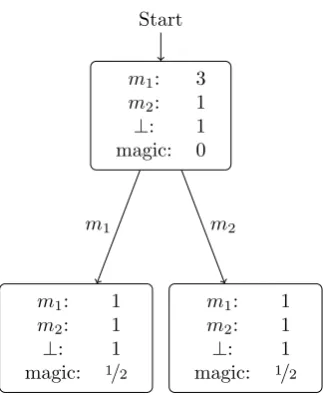
For the sender, there is a start urn for each state containing the following balls:
message balls for each possible message
terminal balls to finish a message sequence
magic balls to expand a node
m1: 3
m2: 1
⊥: 1 magic: 1
[image:18.595.262.333.183.266.2]Start
Figure 3.2: Sender tree for a single state before expansion of the start node
m1: 3
m2: 1
⊥: 1 magic: 0
m1: 1
m2: 1
⊥: 1 magic: 1/2
m1
m1: 1
m2: 1
⊥: 1 magic: 1/2
m2
Start
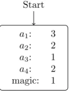
[image:18.595.216.378.425.623.2]a1: 3
a2: 2
a3: 1
a4: 2
[image:19.595.262.334.128.221.2]magic: 1 Start
Figure 3.4: Receiver tree before expansion of the start node
3.2.3
Receiver
The receiver starts with a single urn containing the following balls:
action balls for each action
magic balls for expanding nodes
In the initial configuration, the receiver does not listen to any messages from the sender and draws a ball immediately. In a four action situation this will result in an average payoff of 0.25 (figure 3.4). When the magic ball is drawn, the receiver will start listening to the next part of the message if this is available. The start node will expand by generating children nodes for each possible message (figure 3.5). In the child nodes the balls of the parent node are copied, except the magic ball which is divided over the children.
By copying the contents of the parent node to the children, the receiver uses the available information. Suppose the agents have developed a system with only length 1 messages for a four state game. Some information is transferred, for example thatm1indicatess1ors2and the node for [m1] will have more balls
for a1 and a2. When the agents start using longer messages, it is most likely
that the messages starting withm1will be indicatings1ands2. By copying the
contents of the parent node, the probability of selectinga1 ora2 will be more
likely in the nodes for [m1, m1] and [m1, m2]. If a new urn would be used, all
action would be equiprobable and the information that is already in the system would not be used.
After a branch of the tree is developed, the receiver will always use this if the signal is long enough. Once the choice is made to listen to a part of the signal, the receiver will always do this.
3.2.4
Variations on the basic model
a1: 3
a2: 2
a3: 1
a4: 2
magic: 0
a1: 3
a2: 2
a3: 1
a4: 2
magic: 1/2
m1
a1: 3
a2: 2
a3: 1
a4: 2
magic: 1/2
m2
[image:20.595.215.378.128.345.2]Start
Figure 3.5: Receiver tree for a single state after expansion of the start node
Updating incomplete messages for the receiver
In the basic receiver model, only the urn that is used for the decision is updated. Consider a signalling system for a four state game where [0,0] indicates state 1 and [0,1] indicates state 2. What would it mean if the receiver hears [0]? It could be that the sender is uncertain whether state 1 or 2 is the case. Another option is that the sender actually sent [0,0] or [0,1], but there is noise and the receiver only heard the first part.
In the current framework the sender has perfect information of the state and the receiver hears the message perfectly. It is still possible that the sender uses [0] once in a while, because all urns contain terminal symbols.
For the receiver only the urns for [0,0] and [0,1] are updated and urn [0] might contain balls of all types. If the magic balls were used very early in the learning process and the agents started using longer messages from the begin-ning, the urn [0] was updated only a few times. If all actions are equiprobable, the expected payoff is 0.25. But the sender uses messages starting with 0 only for states 1 and 2. By updating the urns the receiver passes while parsing the message, the expected payoff can be 0.5.
If a node receives payoffpfor actiona, its parent node receives payoffrpfor a feedback rater and updates actionawith this payoff (figure 3.6). This way, the initial messages of the signals will have meaning on their own and not only in combination with the other messages in the signal.
Updating with state similarity
[ ]
[m1]
[m1, m1]
m1
[m1, m2]
m2
m1
[m2]
m2
Start
Update actionawithp
Update actionawithrp
[image:21.595.158.443.126.323.2]Update actionawithr2p
Figure 3.6: Receiver tree with extra update on parent nodes. After receiving message [m1, m1] the receiver performed action
a with payoff p. The node for this message is updated in the usual manner and the parent nodes will be updated with rater.
systematic system composition will occur more often. This allows the agents to communicate about states that have not been reinforced, but are similar to states that have occurred in the past. In normal reinforcement learning the updates only influence the states that are used. By spill-over reinforcement learning [6] similar states will be updated as well.
If a state-action combination resulted in payoff, similar states will be rein-forced as well. Each state will be updated with payoff proportional to their similarity with the state that was actually used. The similarity with states is between 0 (no similarity) and 1 (the state itself, possibly indistinguishable other states) and given as a vector. In figure 3.7 an example can be seen. For all states that have some similarity with the actual state, the path of the message that was used is reinforced.
For the receiver the actions will be updated according to similarity. For a matching game we assume that for two states sn, sm their respective optimal actions an, am have the same similarity as the states. If actiona1 resulted in
payoffp, actiona2with similarityqwill be updated withpq.
If the parent nodes of the final node are updated as well, these two measures will be combined. Ifa1was used node [m1, m1] and the parent nodes are updated
with rater, thena2 will be updated in [m1] with pqr.
Updating with message similarity
s1 s2 s3 s4
[image:22.595.89.507.122.254.2]Update withp Update withpq No update Update withpr
Figure 3.7: Sender trees for updating according to state sim-ilarity. Sending [m2, m1] in state 1 resulted in payoff p. The
similarity of the states with respect to s1 is [1, q,0, r] and the
trees for the states are updated accordingly.
not necessary: The choice of messages in the branches of the tree is independent for the siblings. If the agents would use a prefix to indicate a property like “nearby” or “far away”, the choice of signals for the predators would differ depending on the prefix.
Therefore signals will be updated according to similarity. If two signals end with the same message, there is some degree of similarity. This degree depends on parametersand how much the signals have in common. If two signals have distancento a common ancestor node, the similarity issn−1 (figure 3.8).
3.3
Methods
The sender starts with one magic ball, one terminal ball and one message ball for each message. The receiver starts with one magic ball and one action ball for each action.
The simulations for the basic model were done with 103 trials per setting
and 106 steps per trial. The agents played a Lewis signalling game with n
equiprobable states and an equal number of actions.
A run is considered failed if the average payoff over the 106 plays is 0.8 or less. The results are compared with the Barrett-Skyrms model[2] and normal urn learning.1
The variations on the basic model were only tested for 100 trials in a four state , 2 message game. Each trial had 106 plays. Some trials used costly
messaging. For each message in the signal cost c was subtracted from the payoff. No negative payoffs were given, the minimum payoff was 0.
1In Barrett’s papers the results for the multiple sender model are compared to regular urn
Start
[image:23.595.188.405.125.295.2]1 s s2 s2
Figure 3.8: Updating according to similarity of the signals. Only signals with the same length and same end message have this similarity.
Number of states n Automaton model with 2 messages
Automaton model withnmessages
Urn learning withn
messages
3-state 0.004 0.001 0.1
4-state 0.054 0.002 0.187
[image:23.595.98.495.356.419.2]8-state 0.068 0 0.064
Table 3.2: Failure rates for signalling games
3.4
Results
Table 3.2 shows that the basic model is results in successful signalling systems. The results are better if there are more messages available, but with only two messages the model performs better or the same as regular urn learning. The automaton model is less likely to end in a pooling trap, as can be seen in table 3.3.
It seems that the empty message, that is allowed in the basic model, influ-ences the results. For the variation without empty messages pooling occurred only in 1 out of 100 trials for the four message variant.
The resulting strategies do not follow a clear pattern. In figure 3.9 the strategies for a sender and receiver of a successful run of a four state, 2 message game without empty messages. For the sender 100 messages for each state were collected. For the receiver, 100 action choices for each possible message with maximum length 3 were collected. Not each strategy for the receiver is representative. Message [1,1,0] is rarely used by the sender and few updates have been done for this message. In this strategy the sender uses messages that start with 0 for three states, while messages staring with 1 are mostly used for a single state. This pattern is very common in the basic model.
Success rate in-terval 2-message automaton 8-message automaton Barrett’s 2-term/3-sender model 8-term urn learning
[0.0,0.5) 0.0 0.0 0.0 0.0
[0.5,0.625) 0.004 0.0 0.001 0.0
[0.625,0.75) 0.048 0.0 0.081 0.047
[0.75,0.875) 0.404 0.01 0.589 0.545
[image:24.595.93.499.151.249.2][0.875,1.0] 0.544 0.99 0.329 0.408
Table 3.3: Distribution of signal success rate for 8-state/8-action games
0 20 40 60 80 100
[0] [0,0] [0,0,0] [0,0,1] [0,1] [0,1,0] [0,1,1] [1] [1,0] [1,0,0] [1,0,1] [1,1] [1,1,0] [1,1,1] other
Number of runs sender
0 20 40 60 80 100
[0] [0,0] [0,0,0] [0,0,1] [0,1] [0,1,0] [0,1,1] [1] [1,0] [1,0,0] [1,0,1] [1,1] [1,1,0] [1,1,1]
Number of runs receiver
[image:24.595.53.571.341.629.2]Cost Average Payoff Relative Payoff Average length Failure Rate
0 0.991 0.991 2.61 0.01
0.05 0.884 0.955 2.185 0.02
0.1 0.814 0.958 1.818 0
0.2 0.675 0.964 1.545 0.05
The relative payoff with respect to the maximum possible payoff for costly signalling. The agents will learn to signal with shorter messages if the costly signalling is used.
Feedbackrate Average Payoff Average Length Failure Rate
0 0.991 2.61 0.01
0.1 0.982 2.65 0.0
0.25 0.959 2.76 0.02
0.5 0.936 2.89 0.03
Updating the parent nodes has a slight negative effect on the success and results in longer messages.
p q Average Payoff Average Length Failure Rate
0 0 0.991 2.61 0.02
0.1 0.1 0.724 2.60 1.0
0.25 0.25 0.463 2.63 1.0
0.1 0.25 0.571 2.64 1.0
[image:25.595.152.438.325.387.2]Results for spillover between states with a simple payoff matrix.
Table 3.4: Results for the variations of the basic model.
Introducing cost leads to shorter signals, which is expected. When agents use shorter signals, fewer nodes are used and these will be trained more and converge faster. This can be seen in the figure.
Updating the parent nodes for the receiver results in longer messages and slightly lower payoff in the noise free environment. However, strategies like figure 3.11 are more common. These strategies are more systematic and will most likely have better results in an environment with noise.
The resulting signalling systems are not compositional. It is not the case that similar states are consistently indicated by the same message at the same position. This makes it unlikely that successful creative compositionality will occur for models with these variations and parameters. If a state is not rein-forced, but is similar to other states that have been reinrein-forced, the chance of successful communication is still small.
0 0.1 0.2 0.3 0.4 0.5 0.6 0.7 0.8 0.9 1
·106
0.76 0.78 0.8 0.82 0.84 0.86 0.88 0.9 0.92 0.94 0.96 0.98 1
steps
relativ
e
pa
y
off
Structured payoff Cost Baseline
Feedback to parent nodes
[image:26.595.93.511.211.589.2]‘
Figure 3.10: Average success rate during 25 trials for four vari-ations on the model. The structure of the payoff i p = 0.25,
0 20 40 60 80 100 [0]
[image:27.595.53.561.272.548.2][0,0] [0,0,0] [0,0,1] [0,1] [0,1,0] [0,1,1] [1] [1,0] [1,0,0] [1,0,1] [1,1] [1,1,0] [1,1,1] other
Number of runs sender
0 20 40 60 80 100
[0] [0,0] [0,0,0] [0,0,1] [0,1] [0,1,0] [0,1,1] [1] [1,0] [1,0,0] [1,0,1] [1,1] [1,1,0] [1,1,1]
Number of runs receiver
Chapter 4
Neural Networks
4.1
Introduction
The models in the previous chapter were not very good at generalising over structured state spaces. In basic reinforcement learning the agents will only learn for the states that actually occurred and will not use any connection with other states. The variations on the models were an attempt to solve this, but it was not very successful.
A computational model that is very good at recognising patterns is the ar-tificial neural network. These networks are inspired by the structure of neurons in the brain. Artificial neural networks consist of layers of nodes in a weighted network. The nodes receive input and will be activated if the input exceeds a threshold. The activated nodes will in turn determine the input of the nodes they are connected to. The final layer, the output layer, will determine which action is chosen.
Artificial neural networks learn by training and are very suitable for su-pervised learning tasks where a training set of stimuli with correct answers is available. After training, the network is able to predict the outcomes for similar stimuli. An application of this would be handwriting recognition. The input is the pixel information of handwriting and the output is a character.
This is very different from the unsupervised learning task of playing sig-nalling games. Not only are there multiple sigsig-nalling systems possible, the only feedback the agents have is payoff.
second, the players could be in any environment and receive information on the environment.
In both settings, the agents learn to cooperate in environments with mainly stag hunt games and defect in environments with a higher probability of playing prisoners dilemma.
Important in this setup is what the output nodes represent: the expected payoff of choosing an action. The choice for an action is made based on these values and the network will learn by updating the outputs with the payoff that was actually received.
We want to explore a similar setup for agents playing signalling games. An important difference will be the type of input: in the strategic game setup, the agents have the same role and receive the same input. This input represents the same environment during the entire session. The agents play against a random player each round and do not know which. The agents have no information on the action of their opponent, their only feedback is the received payoff. The agents will learn the a strategy for each environment, this depends on the strat-egy of the other players.
The signalling games are with two fixed agents that have different roles, sender and receiver. They will only learn from each other. The receiver is only informed of the choice of message of the sender, which can refer to a different state in every turn. The sender receives no feedback on the interpretation of the receiver and the receiver does not learn which state the sender referred to.
In both games, the players are not informed of possible payoffs of the options that were not used.
4.2
Technical framework for simple Lewis game
4.2.1
Environment
In the simple game, a single state, message and action is used each round. These items are represented by binary vectors with exactly one 1. For example, state [0,0,1,0] representss3in a four state game.
Each round of the game has the following steps:
• A state is selected according to the state probability vector
• The sender generates a message
• The receiver selects an action for the message
• If the state and action match, the agents get payoff 1, otherwise 0. Both agents update the weights of their network according to this payoff
4.2.2
Agents
The agents are feed forward neural networks (schematic representation in fig-ure 4.1). The setup is the same for both sender and receiver, only the number of input and output elements might differ.
The input layer gets activated by a vector. This activates the hidden layer according to the weights of the connections. Before training, these weights are set at random values.
Hj=σ(
X
i
W0j,i·Ii+bi0)
Hereσ is the logistic sigmoid function. This function mapsR→(0,1) and is a threshold function.
σ(X) = 1 1 + exp(−x)
The output layer is activated by a linear function. The output layer will represent the expected payoff from each action and therefore the values will be in R.
Ok=
X
j
W1k,j·Hj+bk1
For the sender, the number of input and output nodes is equal to the number of states and messages, respectively. For the receiver, the number of input and output nodes are equal to the number of messages and actions, respectively. For both agents, the size of the hidden layer is twice the size of the input layer. The size of the hidden layer is related to the complexity of the function the agents will learn. To categorise data points that are divided by a linear function only a few hidden layer nodes are needed, or even none. If the function that needs to be learned is more complex, more hidden layer nodes are necessary.
For both agents, the output nodes will represent the expected payoff of choos-ing this action. These expected payoffs are translated to action probabilities by the softmax function:
P(ai) = Pexp(Oi/τ)
jexp(Oj/τ)
The temperature τ influences the exploration. In reinforcement learning the agent should explore all possible actions in the beginning, with possible suboptimal payoff. After sufficient exploration, the agent should always use the action with the highest expected payoff. Initially, the game is played with high temperature to explore and gradually the temperature is lowered.
For chosen message mn or action an, the agents receive payoff p. Output node On should be the expected payoff. The error in this approximation has to be minimised. This is done by adjusting the weights with a method called backpropagation[11]. The gradient of the squared error e2 is determined and the weights are moved accordingly, scaled by the learning rate. The appropriate learning rate is found experimentally.
..
.
..
.
..
.
I1Ik
B0 H1
H2
Hm
B1
O1
O2
On
p1
p2
pn
b1 0
b1 1
W0m,k W1n,m
Input layer
Hidden layer
Ouput layer
Softmax function
[image:31.595.137.473.262.552.2]Selection probability
4.3
Technical framework for Lewis game with
complex states
4.3.1
Environment
In the complex game, states and actions are not represented by a number but by a vector of their properties. For each game, the number of properties is fixed. Each position in a vector represents a property: if the state has this property, the value is 1, otherwise it is 0. The vector [1,0] represents a state that has property 1 but not property 2 in an environment with 2 properties.
The states are drawn according to a state distribution function. This is independent of the properties: the probability of [1,1] is independent of [1,0] and [0,1]. If necessary, the state distribution can be based on a distribution of the properties, for example probability 0.6 for property 1 and 0.2 for property 2 results in probability 0.12 for state [1,1].
The actions of the receivers are vectors of the same type. The payoffs are specified by a payoff matrix that has an entry for each possible state.
4.3.2
Agents
The agents can send signals that consist of multiple messages. The signals have no syntax, it is a set of words without structure. To achieve this, the number of output nodes is doubled. Each pair of output nodes represents a message : one node estimates the expected payoff of using this message, the other node the payoff of excluding it. The softmax function is applied pairwise, resulting in a probability for each message. For each message this probability is used to determine whether it is part of the signal. The signal is represented as a binary vector where 1 indicates that a message is used. [1,0,1] represents messages 1 and 3 being used and message 2 being left out.
The receiver will select properties of actions in the same manner as the sender selects messages for the signal. The setup of the network is visualised in figure 4.2.
4.4
Methods
The neural network was implemented in the PyBrain machine learning library for Python [13].
Unless otherwise specified, the agents played a signalling game with the same number of states, messages and actions (simple) or the same number of state properties and messages (complex).
For each run, the weights of the networks were set randomly. The trial consists of two phases: learning and testing. The number of learning steps depends on the number of states to keep the number of training steps in the same order for every state. This was set at 1000 steps per state. After training, the system is tested for 1000 steps without updating.
..
.
..
.
..
.
..
.
I1Ik
B0 H1
H2
Hm
B1
O1
O2
O2n−1
O2n
p1
pn
b1 0
b1 1
W0m,k
W12n,m
Input layer
Hidden layer
Ouput layer
Softmax function
[image:33.595.137.473.261.551.2]Selection probability
states temperature minimum average failure decrease temperature success rate
2 0.06 0.03 0.997 0.005
3 0.03 0.03 0.962 0.11
4 0.015 0.06 0.938 0.235
[image:34.595.172.423.125.199.2]8 0.01 0.06 0.846 0.305
Table 4.1: Succes rates for the simple Lewis game
vary per game and are determined experimentally. Due to the many possible variations in these settings, it is not certain that these values are optimal.
The temperature decrease is an important variable in playing signalling games. Before training, some choice options have much lower expected pay-off than others due to the random assignment of the weights. If the network has a short exploration period, these seemingly unprofitable choices are rarely used. In the test setting the agents had exactly enough messages to avoid pooling states and not using some messages will result in pooling and lower payoffs.
In high temperature, the choice probabilities are almost equal. If the net-works stay too long in this exploration phase, the expected payoff will be equal for all choices: 1/n fornoptions. When the temperature decreases, the choice probabilities will remain almost equal and the agents will continue to act ran-domly. It is important that the agents explore all options, but also settle on a convention quickly.
The data is collected for 200 runs per setting. A run is considered failed is the average payoff over the test steps is less than 0.8.
To analyse the pooling behaviour, the test results are classified with respect to the expected payoffs of pooling equilibria. This indicates the number of inefficient used messages. The precise form of pooling is not determined. For example, an eight state game with three states pooled together has the same expected payoff as the same game with two states pooled together twice. A four state game with payoff 0.8 is classified as using 1 state inefficiently because it is closest to expected payoff of 0.75.
For the complex experiments, the resulting signalling system was tested for compositionality. For this the following definition was used: a signalling system is compositional iff for every pair of completely distinct states, the sender uses completely distinct messages.
4.5
Results
4.5.1
Simple game
states Number of inefficient messages
n 0 1 2 3 4
2 .995 0.005 - -
-3 0.89 0.11 0 -
[image:35.595.199.396.125.199.2]-4 .765 0.235 0.0 0.0 -8 .165 0.52 0.26 0.05 0.005
Table 4.2: Percentage of pooling for the simple Lewis game.
states Reinforcement Learning Neural Networks
Failure rate Signalling systems Failure rate Signalling systems
4 0.187 0.835 0.185 0.815
8 0.064 0.408 0.385 0.615
16 0.03 ≈0.072 0.405 0.515
Table 4.3: Comparison for basic RL and neural networks with complex states. Data for 16 state RL from [4]
4.5.2
Complex game
Purely based on the failure rates and average payoff the neural network also performs worse on the complex games (table 4.3). That is, basic reinforcement learning is more likely to have an average payoff of at least 0.8.
For games with more states several of the pooling equilibria result in a payoff >0.8 and are considered a success. Signalling systems become rare for reinforcement learning when the number of states goes up. Only approximately 7% of the 16-state games ends in a signalling system.1 This is not the case
for neural networks: over half of the networks learn a signalling system for the 16-state game and even more for the game with less states. All of the signalling systems are compositional, they have completely distinct messages for completely distinct states.
In this first experiment the available number of messages is minimal: it is not possible to have signalling system with less messages. With extra messages it is not necessary to use all combinations. In table 4.4 is shown that extra messages do not influence the success of the system much.2 The successful trials do not necessarily have a compositional signalling system.
4.5.3
Creative compositionality
Compositional language is particular useful in situations where the agents have not seen a particular stimulus before, but there is similarity with previously encountered stimuli. This situation is simulated by omitting one or more states
1In Barrett’s work [4] the proportion of games that is in the [0.95,1] payoff interval is given,
this is 0.072. In theory this is equal to the proportion of signalling systems.
2These trails have temperature decrease and minimum temperature 0.06 and a hidden
[image:35.595.124.470.243.316.2]properties messages average payoff failure rate signalling systems compositionality
2 3 0.891 0.295 0.705 0.37
2 4 0.911 0.275 0.725 0.17
3 6 0.718 0.545 0.335 0.02
[image:36.595.92.504.125.187.2]3 8 0.724 0.57 0.345 0
Table 4.4: Success rates for games with extra messages
0 0.2 0.4 0.6 0.8 1 0
0.5 1
Training result
T
est
result
0 0.2 0.4 0.6 0.8 1 0
0.5 1
Training result
T
est
result
Figure 4.3: Payoff for a single missing state in games with 2 (left) and 3 (right) properties
from the training data. After training, the system was tested only on the missing states without updating the weights of the network.
In figure 4.3 can be seen that networks that have more success on the training set are also more likely to use new signals successfully.
If the previously untrained states have at least 0.8 payoff over the test steps, we consider the creative composition successful. We consider this only for the runs that had at least 0.95 payoff on the training set.
In table 4.5 can be seen that the structure of the training set is important. If two states are untrained, but have no overlap in properties, the performance is not much worse than when a single state is untrained. When there is more overlap between untrained states, it becomes very hard to communicate about these states.
[image:36.595.98.504.217.377.2]Properties Messages Missing states Creative success
2 2 [0,0] 0.43
2 2 [0,0], [1,1] 0.19
3 3 [0,0,0] 0.95
3 3 [0,0,0], [1,1,1] 0.80 3 3 [0,0,0], [0,0,1] 0.22 3 3 [0,0,0], [0,0,1], [1,1,1] 0.17
3 4 [0,0,0] 0.33
3 4 [0,0,0], [1,1,1] 0.23 3 4 [0,0,0], [0,0,1], [1,1,1] 0.05
Chapter 5
Conclusions and further
work
5.1
Conclusions
The models that have been presented in this thesis each have their advantages. The automaton model is more successful than regular reinforcement learning. It does not have a fixed message length, but the length of the sequence is arbitrary. This allows for arbitrary many signals from a small set of basic messages. However, the resulting signals are not compositional.
In the neural network model truly compositional systems will emerge for the majority of the trials. The neural network is also able the generalise over the properties of the states and use this for new states. If the neural network does not succeed in learning a signalling system, the results are worse than for reinforcement learning.
5.2
Further work
The systems that were presented in this thesis have been tested in specific setups: a single sender and a single receiver that communicate about a finite set of equiprobable states.
It is important to know how these models will work in a multi agent exper-iment. Will the agents learn to communicate if they do not always play with the same opponent? Two agents can coordinate their strategies and develop a signalling system, but will this also be true for a (small) population of agents? In the most basic form this can be tested by creating a population of new agents and seeing what strategies emerge. Another option is a version in which new agents are introduced in a population of agents that are already trained. If the agents are slowly replaced by new agents, strategies that are easier to learn will make up a bigger proportion of the population.
would expect that they can communicate about states that are rarely seen. The question remains: will a compositional signalling system develop for states that are not equiprobable? Also, will there develop some pragmatic “smartness” for stereotypical states? If 80% of the elephants is grey, it would be easier to just call them elephants and only add an extra signal if this is not the case. Only the rare pink elephants would be indicated with a longer signal that makes the colour explicit.
Bibliography
[1] Raffaele Argiento, Robin Pemantle, Brian Skyrms, and Stanislav Volkov. Learning to signal: Analysis of a micro-level reinforcement model. Stochas-tic Processes and their Applications, 119(2):373 – 390, 2009.
[2] Jeffrey A. Barrett. Numerical simulations of the lewis signaling game: Learning strategies, pooling equilibria, and the evolution of grammar. UC Irvine Institute for Mathematical Behavioral Sciences Preprint, 2006. [3] Jeffrey A. Barrett. Dynamic partitioning and the conventionality of kinds.
Philosophy of Science, 74:527–546, 2007.
[4] Jeffrey A. Barrett. The evolution of coding in signaling games.Theory and Decision, 67:223–237, 2009.
[5] Daniel Cownden, Kimmo Eriksson, and Pontus Strimling. Bounded ratio-nality and perception: strategies for a confusing world. In Games, Inter-active Rationality, and Learning (GIRL’13LUND), 2013.
[6] Michael Franke. Creative compositionality from reinforcement learning in signalling games. In The Evolution of Language: Proceedings of the 10th International Conference (Evolang 10), pages 82–89, 2014.
[7] David Lewis. Convention: A Philosophical Study. Harvard University Press, 1969.
[8] Karim Ouattara, Alban Lemasson, and Klaus Zuberb¨uhler. Anti-predator strategies of free-ranging campbell’s monkeys. Behaviour, 146(12):1687– 1708, 2009.
[9] Karim Ouattara, Alban Lemasson, and Klaus Zuberb¨uhler. Campbell’s monkeys concatenate vocalizations into context-specific call sequences. Pro-ceedings of the National Academy of Sciences, 2009.
[10] Alvin E. Roth and Ido Erev. learning in extensive form games: experimen-tal data and simple dynamic models in the intermediate term. Games and Economic behaviour, 8:164–212, 1995.
[11] David E. Rumelhart, Geofrey E. Hintont, and Ronald J. Williams. Learning representation by back-propagating errors. Nature, 37(1):20–29, 1986. [12] Sue Savage-Rumbaugh, Kelly McDonald, Rose A Sevcik, William D
[13] Tom Schaul, Justin Bayer, Daan Wierstra, Yi Sun, Martin Felder, Frank Sehnke, Thomas R¨uckstieß, and J¨urgen Schmidhuber. PyBrain. Journal of Machine Learning Research, 11:743–746, 2010.
[14] Brian Skyrms. Signals. Oxford University Press, 2006.
[15] J. Maynard Smith and G.R. Price. The logic of animal conflict. Nature, 246:15–18, 1973.
[16] Tianming Yang and Michael N. Shadlen. Probabilistic reasoning by neu-rons. Nature, 447:1075–1080, 2007.