Solid Earth change and the evolution
of the Antarctic Ice Sheet
Pippa L. Whitehouse
1, Natalya Gomez
2, Matt A. King
3&
Douglas A. Wiens
4Recent studies suggest that Antarctica has the potential to contribute up to ~15 m of sea-level rise over the next few centuries. The evolution of the Antarctic Ice Sheet is driven by a combination of climate forcing and non-climatic feedbacks. In this review we focus on feedbacks between the Antarctic Ice Sheet and the solid Earth, and the role of these feed-backs in shaping the response of the ice sheet to past and future climate changes. The growth and decay of the Antarctic Ice Sheet reshapes the solid Earth via isostasy and erosion. In turn, the shape of the bed exerts a fundamental control on ice dynamics as well as the position of the grounding line—the location where ice starts tofloat. A complicating issue is the fact that Antarctica is situated on a region of the Earth that displays large spatial variations in rheo-logical properties. These properties affect the timescale and strength of feedbacks between ice-sheet change and solid Earth deformation, and hence must be accounted for when considering the future evolution of the ice sheet.
T
he solid Earth, along with the oceans and the atmosphere, exerts a strong influence on the dynamics of the Antarctic Ice Sheet (AIS). The pre-glacial topography of the Antarctic continent determined the location and style of glacial inception ~34 Ma ago1, whereas today the shape of the bed and the properties of the ice-bed interface exert afirst-order control on the contemporary pattern of iceflow2. In the intervening period the bed of the AIS has been continuously reshaped by erosion and sedimentation, periodicallyflexed by glacial isostasy, and abruptly altered by tectonic and volcanic activity, with the latter two processes also playing a role in determining the thermal conditions at the bed (Fig.1). Basal heatflux affects iceflow via its influence on subglacial hydrology and ice rheology3, but its spatial variation is currently poorly quantified4. Parts of Antarctica are underlain by active volcanoes, notably West Antarctica (Fig.1). This is of interest because in other regions, e.g., Iceland5, volcanism has been shown to increase during periods of deglaciation. However, little is known of this phenomenon in Ant-arctica6and a detailed review of this effect is therefore not possible. We instead focus on those processes that are better known and that control long-wavelength changes to the shape of the bed beneath Antarctica–glacial isostasy and erosion–and feedbacks between these processes and ice sheet evolution.Interactions between ice sheets and the solid Earth have long been studied within thefield of Glacial Isostatic Adjustment (GIA)—defined here as the response of the solid Earth and the
https://doi.org/10.1038/s41467-018-08068-y OPEN
1Department of Geography, Durham University, Durham, UK DH1 3LE.2Department of Earth and Planetary Sciences, McGill University, Montreal H3A 0E8,
Canada.3School of Technology, Environments and Design, University of Tasmania, Hobart, TAS 7001, Australia.4Department of Earth and Planetary Sciences, Washington University, St Louis, MO 63130, USA. Correspondence and requests for materials should be addressed to
P.L.W. (email:[email protected])
123456789
global gravity field to changes in the distribution of ice and water on Earth’s surface. The first numerical models of GIA were developed in the 1970s7 but they have received renewed attention over the last decade, reflecting the important role they play in the interpretation of satellite measurements of contemporary ice-sheet change8. A number of recent studies have also sought to understand the strength of feedbacks acting in the opposite direction, that is, the impact of solid Earth deformation on ice dynamics and the potential for this defor-mation to delay or prevent unstable ice-sheet retreat9,10. Such feedbacks were first considered in the 1980s11 but have only recently begun to be implemented into fully-coupled models12, where the evolving shape of the solid Earth and the depth of the ocean adjacent to an ice sheet grounded below sea level act as fundamental boundary conditions on the dynamics of the ice sheet.
The strength of any feedbacks between glacial isostasy and ice dynamics depends on the rate at which the solid Earth responds to ice-sheet change, which, in turn, depends on the rheological properties of the mantle. Seismic evidence13 indi-cates that there are significant spatial variations in mantle properties beneath Antarctica, which suggests mantle viscos-ities, and hence relaxation timescales, may vary by up to several orders of magnitude from the global mean. Indeed, in the northern Antarctic Peninsula, geodetic evidence14suggests that contemporary ice loss is triggering a viscous response orders of magnitude more rapidly than was previously assumed possible in Antarctica – on decadal rather than millennial timescales. Feedbacks on ice dynamics are likely to be enhanced in such regions15, and the ongoing GIA signal is likely to be dominated by recent ice-sheet change (few millennia or less), as opposed to the ice loss that followed the Last Glacial Maximum (LGM)16. Here, we define the GIA signal to be the ongoing response of the solid Earth, the gravityfield, and/or relative sea level to past ice-sheet change.
The growth and decay of the AIS is driven by a combination of climate forcing and non-climatic feedbacks, but modelling studies that seek to understand the controls on AIS change often neglect to consider how the ice sheet alters its own boundary conditions. Over the timescale of the last deglaciation, GIA model output17,18 suggests that the response to surface load change can alter bed slopes across West Antarctica by 0.25–0.4 m/km (values may be an underestimate due to assumptions of strong mantle rheology) and that water-depth change around the margin of the ice sheet can deviate from eustatic by >100 m. Coupled ice sheet-sea level models can now be used to quantify the impact of such changes on ice sheet evolution15,19. Over timescales of millions of years, changes to the shape of the ice sheet bed will additionally reflect processes associated with erosion and deposition, the isostatic response to sediment redistribution, and mantle con-vection. Feedbacks between ice sheet evolution and long-term landscape evolution have been hypothesised20, but they have not been modelled within a coupled framework. The impacts of long-wavelength isostasy-driven changes to ice sheet boundary conditions are reviewed here, but smaller-scale subglacial controls, such as the material properties of the bed and variations in subglacial hydrology and geomorphology, are discussed elsewhere2.
In this review we proceed by briefly summarising the current state of knowledge on ice-sheet change and glacial isostasy across Antarctica, before discussing the impact of spatial variations in Earth rheology on glacial isostasy and the impact of GIA on ice dynamics. Feedbacks between ice sheet and landscape evolution are discussed, and we conclude by identifying a number of future research priorities that link ice history, Earth rheology, and the overarching issue of global sea-level change.
Antarctic ice-sheet change and glacial isostasy
Forward model predictions of GIA-related solid Earth deforma-tion, gravity-field change, and polar motion rely on: a recon-struction of the spatial and temporal pattern of past ice loading, a viscoelastic Earth model that describes the time-dependent response of the solid Earth to surface loading changes, and the iterative consideration of physical feedbacks associated with polar motion and coastline position as they are altered by the defor-mation of the solid Earth and the gravity field21,22. While the third component is well defined by physical theory, Antarctic ice-sheet reconstructions and solid Earth rheology are subject to substantial uncertainty and debate.
GIA modelling can be used to infer past large-scale ice-sheet change via comparison of model output with a range of constraint data relating to sea-level change and solid Earth deformation18,23. On a global scale, such data-model comparisons have been used to estimate the timing of ice-sheet growth and retreat over glacial cycles24,25, but the combined dependence of model output on Earth rheology and ice history leads to non-uniqueness26, and it remains challenging to determine how ice was partitioned between the different ice sheets27.
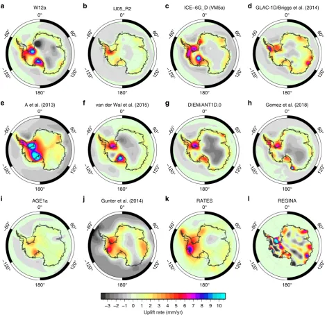
Reconstructions of the LGM AIS suggest an ice sheet larger than present, equivalent to ~5–22 m global mean sea level28. This range reflects differences in methodology and the interpretation of data constraints. The most common reconstruction approaches con-sider either numerical models of ice-sheet dynamics19,29or local geological, geomorphological, and geodetic data constraints on past ice extent30, or a hybrid31,32. Data constraints are sparse as they rely on sampling of spatially limited bedrock exposures33,34 or interpretation of ice core records35, while numerical ice-sheet models are restricted by a limited representation of reality. Continent-wide ice-sheet reconstructions can be produced by simulating the response of dynamic models to past climate changes19,31,36–38, but at present there is not enough data to tightly constrain such models. Consequently, there is significant variation in the predicted magnitude and spatial pattern of isostatic defor-mation across Antarctica due to past ice-sheet change39(Fig.2).
It is important to note that some of the differences in Fig.2 reflect the timescale of ice-sheet change considered to contribute to the deformation signal; traditional forward models of GIA do not consider ice-sheet change during the last millen-nium (Fig.2a-f), but this is accounted for in solutions derived via coupled modelling (Fig. 2g, h) or data inversion (Fig. 2i-l). Altogether, four approaches to determining the present-day GIA signal are represented in Fig. 2, reflecting a number of recent methodological advances. We do not seek to quantitatively assess the accuracy of each GIA solution, partly due to the difficulty of defining validation data sets, but we briefly note the advantages and limitations of each approach in Table1.
3 4 5 6 7 9 10 Uplift rate (mm/yr)
−3 −2 −1 0 1 2 8
W12a 0°
60°
120°
180°
−120° −60°
IJ05_R2 0°
60°
120°
180°
−120° −60°
ICE−6G_D (VM5a) 0°
60°
120°
180°
−120° −60°
GLAC-1D/Briggs et al. (2014) 0°
60°
120°
180°
−120° −60
A et al. (2013) 0°
60°
120°
180°
−120° −60°
van der Wal et al. (2015) 0°
60°
120°
180°
−120° −60°
DIEM/ANT1D.0 0°
60°
120°
180°
−120° −60°
Gomez et al. (2018) 0°
60°
120°
180°
−120° −60°
AGE1a 0°
60°
120°
180°
−120° −60°
Gunter et al. (2014) 0°
60°
120°
180°
−120° −60°
RATES 0°
60°
120°
180°
−120° −60°
REGINA 0°
60°
120°
180°
−120° −60°
a
e
i j k l
f g h
b c d
Fig. 2Predictions of present-day GIA-related uplift rates across Antarctica derived from forward modelling and data inversion.a–dResults derived using GIA forward models that adopt a 1-D Earth model17,18,30,32,141,145; inban Earth model that reflects low viscosity West Antarctic mantle rheology is used.e,
fResults derived using GIA forward models that adopt a 3-D Earth model55,56; (e) uses the same ice model asc; (f) uses the same ice model asa.g,h
Results derived using coupled ice sheet–sea level models that include ice-sheet change through to present10,87.i–lResults derived from the inversion of
geodetic data42–44,146; note thati–lare reduced in their precision away from data constraints. See original publications for further details Glacial erosion
Offshore deposition
Isostatic uplift Ice sheet retreat
Variable basal heat flux
Variable basal melt
Subglacial volcanism
Interior thickening
Isostatic subsidence
[image:3.595.84.513.51.150.2] [image:3.595.62.534.215.669.2]magnitude of the net Antarctic GIA signal vary over the range ~40–80 Gt/yr45, but basin-level differences remain substantial and in some cases different studies do not even agree on the sign of the mass change in each basin43, which hampers the advance of glaciological insights into the processes governing present change. Differences in estimates of the present-day GIA signal are particularly acute in the region of the Amundsen Sea embayment, where forward models have substantially less GIA signal than inverse solutions. This may be due to the fact that the GIA signal in this low mantle viscosity region predominantly reflects sig-nificant decadal-to-centennial ice load change that is not accounted for in most forward models46,47. For the same reasons, forward models underestimate the signal in the northern Ant-arctic Peninsula, but then so do inverse solutions because the GIA signal in this region has a shorter spatial wavelength than inverse solutions can resolve (~300 km). Comparison of the new gen-eration of GIA models with GPS-derived uplift rates—which must be corrected for elastic deformation associated with con-temporaneous ice-mass change48,49—demonstrates that impor-tant differences remain, notably in West Antarctica and especially in the Amundsen Sea and northern Antarctic Peninsula regions39.
Earth structure and rheology beneath Antarctica
The pattern and magnitude of the solid Earth response to ice-sheet growth and decay is strongly dependent on the rheology of the interior of the solid Earth, and the choice of rheological model has a large effect on the modelled GIA response (see Box1). For example, ice history is often tuned in tandem with Earth rheol-ogy, so adoption of a different rheological model can lead to large differences in the assumed ice history. Earth rheology beneath Antarctica is spatially variable and, as detailed in the next section, this has implications for the behaviour of the ice sheet.
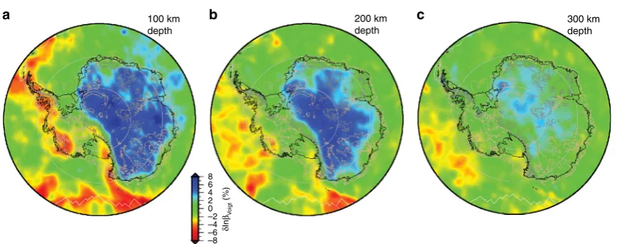
A number of rheological models have been adopted to explain the solid Earth response to surface load change across Antarctica, including linear Maxwell viscoelastic rheology, power law rheol-ogy, and Burgers rheology (see Box1). Regardless of the choice of rheological model, the need for future modelling efforts to con-sider spatial variations in Earth structure beneath Antarctica is now clear. Seismic studies of the upper mantle beneath Antarctica suggest large lateral variations in material properties13,50–53, with greater heterogeneity than observed in areas of Northern Hemi-sphere continental glaciation54. East Antarctica shows high upper mantle seismic velocities characteristic of cold cratonic regions worldwide, whereas West Antarctica shows upper mantle
structure consistent with much warmer tectonically active zones (Fig. 3a-c). The range of seismic velocities observed beneath Antarctica provides strong evidence for lateral variations in mantle viscosity, but absolute values are currently poorly known. Preliminary GIA studies that explore the effect of including lateral variations in mantle viscosity reveal significant differences in predicted patterns and rates of deformation across Antarctica55–58, motivating the need for better constraints on absolute mantle viscosity in this region.
Upper mantle viscosity variations of several orders of magni-tude beneath West Antarctica have been quantified by modelling observed GPS uplift in specific settings. Nield et al.14identified rapid viscoelastic deformation occurring in the northern Ant-arctic Peninsula due to a well-observed change in glacial loading resulting from the 2002 breakup of the Larsen B Ice Shelf. Comparison of GPS time series and modelled uplift in the region suggests upper mantle viscosities of between 6 × 10¹⁷ and 2 × 10¹⁸Pa s in the northern Antarctic Peninsula. Similarly, Zhao et al.59 used the changes in ice load resulting from thinning of Fleming Glacier over recent decades to estimate upper mantle viscosity, 500 km further south along the southern Antarctic Peninsula, to be at least 2 × 10¹⁹Pa s. Other estimates of upper mantle viscosity in West Antarctica include 1–3 × 10²⁰Pa s beneath the southwestern Weddell Sea60and 4 × 10¹⁸Pa s for the Amundsen Sea Coast47. These represent variations of two orders of magnitude. In contrast, estimates of spatially-averaged upper mantle viscosity beneath the whole of Antarctica range from 2 × 10²⁰to 1 × 10²¹Pa s (ref.16,17), which are similar to estimates of upper mantle viscosity in Fennoscandia61. The emerging picture suggests cratonic East Antarctica is characterised by higher upper mantle viscosity than West Antarctica, with exceptionally low upper mantle viscosity, on the order of 1018to 1019Pa s, beneath some regions of West Antarctica.
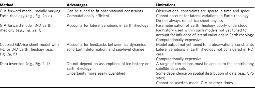
Existing constraints on mantle viscosity across Antarctica draw on our ability to measure the solid Earth response to known surface-load change. In regions where this is not possible, the three-dimensional shear velocity structure of the upper mantle beneath Antarctica can be used to estimate the lateral and depth variation of viscosity. Although there is no direct physical cor-respondence between shear velocity and viscosity, their variation in the upper mantle is largely controlled by temperature62,63. Ivins and Sammis64formulated an approach for converting shear velocity anomalies to viscosity anomalies relative to a global reference 1-D viscosity model, using the observed scaling of shear velocity and density anomalies to infer the temperature scaling, and then using olivine diffusion creep (linear) flow laws to Table 1 Advantages and limitations of four approaches used to determine the present-day GIA signal across Antarctica
Method Advantages Limitations
GIA forward model, radially varying Earth rheology (e.g., Fig.2a–d)
Can be tuned tofit observational constraints Computationally efficient
Observational constraints are sparse in time and space Cannot account for lateral variations in Earth rheology Do not always reflect ice sheet physics
GIA forward model, 3-D Earth rheology (e.g., Fig.2e, f)
Accounts for lateral variations in Earth rheology Parameterisation of Earth rheology poorly understood Ice history used within such models not yet tuned to account for influence of lateral variations in Earth rheology Computationally expensive
Coupled GIA-ice sheet model with 1-D or 3-D Earth rheology (e.g., Fig.2g, h)
Accounts for feedbacks between ice dynamics, solid Earth deformation, and sea-level change
Model output not yet tuned tofit observational constraints Lateral variations in Earth rheology not considered in 1-D case
Computationally expensive Data inversion (e.g., Fig.2i–l) Do not depend on assumptions of ice history or
Earth rheology
Uncertainty more easily quantified
A range of corrections must be applied to the contributing satellite data sets
Some dependence on spatial distribution of data (e.g., GPS sites)
[image:4.595.48.550.71.245.2]constrain the viscosity perturbation. Wu et al.65 proposed a similar method that uses experimentally determined temperature derivatives of shear velocity, including the effect of anelasticity. An alternative method is to estimate the temperature structure of the mantle from the shear velocity structure, and then use a composite rheology that computes the strain associated with both diffusion and dislocation creep mechanisms56. Since the dis-location creep rheology is non-linear, the calculated effective viscosity of the mantle will depend on the stress field. One key assumption in any of these methods is that the observed seismic velocity anomalies result entirely from temperature anomalies, whereas it is well known that a portion of the velocity pertur-bations result from (spatially variable) compositional anoma-lies66. Wu et al.65 adjust their viscosity structure by the percentage of the velocity anomalies thought to be caused by thermal variations, which in their study was estimated to be between 65% and 100%. An alternative approach would involve correcting for (poorly known) spatial variations in mantle composition.
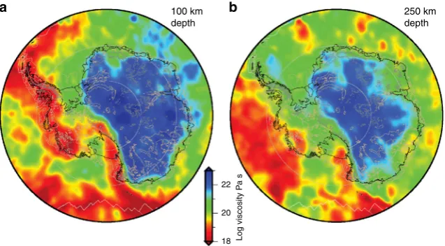
Using the approach outlined in Wu et al.65, the estimated mantle viscosity beneath Antarctica, at depths of 100 and 250 km, varies by 2–3 orders of magnitude across the continent (Fig.4),
with extremely low viscosity predicted beneath the Antarctic Peninsula, the Amundsen Sea coast, Marie Byrd Land, and the Transantarctic Mountain Front. The implications of these visc-osity variations, and in particular the anomalously low viscosities beneath parts of West Antarctica, are explored in the next section.
Feedbacks between GIA processes and ice dynamics It has long been recognised that the evolution of ice sheets is influenced by the geometry and deformation of the underlying solid Earth67, and that the stability and dynamics of marine ice sheets (ice sheets which rest on ground below sea level) are sensitive to the depth of water at their grounding lines, i.e., the point where they begin to float68–70. Marine-terminating ice sheets such as Antarctica lose most of their mass following the flow of grounded ice across their grounding lines intofloating ice shelves (Fig. 5). The ice flux across the grounding line is very sensitive to the thickness of ice there, and the thickness is in turn proportional to the depth of water such that a small increase in water depth at the grounding line leads to a large reduction in grounded ice70. Marine ice sheets are widely thought to be prone to runaway retreat when resting upon beds that slope down towards the interior of the ice sheet, i.e., reverse bed slopes70, as is Box 1 | Rheological models of the solid Earth
The response of the Earth to changing loads has generally been described using a linear Maxwell viscoelastic rheology, with an instantaneous elastic response superposed on a longer-term Newtonian viscous relaxation149,150. The majority of GIA models, including most coupled ice sheet–sea level
models, adopt this simple rheology and consider a spherical Earth, with an elastic lithosphere, a layered viscoelastic mantle, and an inviscid core. Crucially, such models typically include no lateral variation in rheological structure. However, differences in the response of the Earth to surface loading around the world suggest regional variations in rheological properties. Laboratory experiments on mantle materials, primarily olivine, show that the mantle can respond to long-term loading with either diffusion creep, corresponding to linear viscosity, or dislocation creep, corresponding to a power-law viscosity62,151,152. Although both mechanisms operate simultaneously in the mantle, deformation will be controlled by the weaker mechanism at any
given location, with higher stress and larger grain size favouring dislocation creep, i.e., a non-linear response153. It is commonly thought that dislocation
creep dominates at shallow depth in the upper mantle, as indicated by xenoliths154and significant seismic anisotropy155, transitioning to diffusion creep
at depths greater than 200–300 km (ref.152). It is difficult to clearly delineate the regions of the mantle dominated by linear and power-law viscosities
because the rheologies depend on stress and the poorly constrained parameters of water content, grain size and activation volume153. Power-law
rheologies can be introduced into GIA models using a composite rheology, where low stress portions of the model adopt a linear Maxwell rheology and high stress portions adopt a power law rheology assuming some transition stress156. Alternatively, strain is assumed to be the sum of diffusion and
dislocation creep, as calculated using laboratory-basedflow laws assuming parameters such as grain size and temperature56,153,157.
Recent studies show that the transient relaxation following major earthquakes is generally bestfit by a Burgers (biviscous) rheology with two characteristic relaxation times or effective viscosities158,159. These observations have resulted in increased interest in the use of Burgers rheology in GIA
studies27,160. However, similar to the power-law case, there are few data to constrain these more complex models and most recent GIA models
continue to use a Maxwell rheology17,30,32.
100 km depth
a
8 6 4 2 0 –2 –4 –6 δIn
βVo
ig
t
(%)
–8
b 200 km
depth
c 300 km
depth
Fig. 3Spatial variations in Earth properties in the upper mantle beneath Antarctica. Seismic shear wave velocity perturbations at depths of (a) 100, (b) 200 and (c) 300 km beneath Antarctica derived from an adjoint inversion of teleseismic waveforms recorded by seismic stations south of 45°S (ref.52).
Colours indicate observed Voigt average velocity anomalies relative to global reference model STW105 (ref.147). Regions of negative anomalies (slower
[image:5.595.82.516.278.450.2]the case for West Antarctica and much of East Antarctica. This canonical argument is based on the idea that when the grounding line retreats into deeper water, the ice loss at the grounding line increases, leading to further retreat (Fig. 5b). However, this rea-soning does not account for the fact that as ice mass loss occurs, the solid Earth rebounds, and the gravitational attraction of the ice on the surrounding water is diminished, lowering the local sea surface (Fig. 5c). The bathymetry shallows and bed slopes are altered near the margins of the ice sheet where ice mass loss is occurring. Within a modelling framework this local shallowing of water reduces the loss of ice across the grounding line, acting to stabilise the modelled ice sheet71, slowing, and in some cases halting, migration of the modelled grounding line along reverse bed slopes12. Ongoing viscous uplift of the bed following a halt in ice sheet retreat can also initiate readvance of the grounding line in marine areas (e.g., Fig. 6d, ref.15).
Water depth changes can also influence the degree to which ice shelves are able to stabilise the ice sheet. Ice shelves play an important role in the stability and evolution of marine ice sheets by providing resistance to theflow of grounded ice across the grounding line. The spreading of ice shelves is inhibited by friction along their sides and base, particularly where the ice shelf becomes locally grounded on bumps or pinning points in the bathymetry, forming ice rises72. A local decrease in water depth can enhance grounding of the ice shelf at ice rises, stabilising the ice sheet, while an increase in water depth can lead to ungrounding at the ice rise, enhancing flow across the grounding line of the ice sheet. Modelling studies of the AIS have shown that accelerated retreat and thinning and eventually large-scale collapse of marine sectors of the ice sheet can occur when the surrounding ice shelves break up73, but that if ice shelves are able to re-ground, this can have a stabilising effect on the ice sheet74. Furthermore, changes in bathymetry may have implications for ocean circulation and heat transfer under the ice shelves. The role of these and other ice shelf processes in con-trolling the dynamics of the grounded portion of the ice sheet are discussed in more detail in a companion paper by Smith et al. (manuscript submitted).
Initial coupled modelling studies, using simplifiedflowline ice-sheet modelling and bedrock geometry, demonstrated the stabi-lising feedback of sea-level changes on marine ice sheets12,71. Recently, a series of more realistic coupled models have been developed that capture Antarctic ice sheet and ice shelf dynamics,
global sea level and solid Earth deformation, and the interactions between these systems9,10,15,19,36. It has been shown that GIA-related sea-level and solid Earth changes, including changes to the slope of the underlying bed, alter the stressfield of the ice sheet in a way that acts to dampen and slow past19,75and future9,10,76 ice-sheet growth and retreat in Antarctica (Fig.6a, c). An important process that is also accounted for in these coupled models is the feedback between isostatically-driven ice surface elevation change and surface mass balance75,77,78.
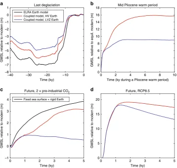
The strength of the feedback between GIA processes and ice dynamics depends on the rheology of the solid Earth. Models representing the palaeo79–81and long-term future evolution of ice sheets over millennia73,82 generally account for ice-load-driven Earth deformation by adopting simplified treatments such as the Elastic Lithosphere Relaxing Asthenosphere (ELRA) model, which treats the asthenosphere as a time-lagged relaxation towards equilibrium11,73,83, or a model with flow in a viscous half-space below an elastic plate82,84. The Earth rheology models adopted in the newly-developed fully-coupled models described above19,36,75 capture more realistically the full multi-normal-mode response of the Earth to both ice and water loading, thus enabling the compu-tation of gravicompu-tationally self-consistent variations of the sea surface, and Earth rotational effects. By solving the sea-level equation7, these studies also account for migrating shorelines, including migration into regions previously occupied by marine-based ice. Ice model simulations15over the last deglaciation incorporating an ELRA bed model (black line) and the full sea-level coupling (blue and red lines) are shown in Fig.6a. Note that the bed topography at the start of each simulation shown in Fig.6a will be different; this is to ensure that thefinal modelled topography is close to the modern observed topography in each case. Due to the complexity and spatial varia-tions of bedrock geometry, ice dynamics and climate-ice interac-tions, the importance of GIA processes on ice sheet evolution cannot be quantified universally and must be considered on a case-by-case basis for different regions, time periods, and climate forcings.
When considering short-term change, ice-sheet models designed to simulate decadal to centennial-scale transient ice dynamics in response to future warming85,86often do not include bedrock deformation and sea-level changes. Simulated Antarctic ice volume changes under moderate future climate warming with fixed bed and sea surface are compared with results from a coupled model9 in which these surfaces are allowed to vary (Fig. 6c). The impact of sea-level changes on ice dynamics has 100 km
depth
22
Log viscosity P
a
s
20
18
a b 250 km
depth
Fig. 4Spatial variations in estimated upper mantle viscosity beneath Antarctica at depths of (a) 100 km and (b) 250 km. Viscosity is estimated using the seismic shear velocity model presented in Fig.3and the method outlined in Wu et al.65, as discussed in the text. These results are derived using a dry
diffusion creep rheology62and the IJ05-R2 (ref.30) reference viscosity model, assuming that the seismic velocity variations are entirely due to
[image:6.595.139.458.51.227.2]previously been considered negligible on these timescales, in particular under strong warming, because the viscous response of the Earth is only considered relevant on millennial timescales and longer. However, as discussed above, the Earth structure under-neath the AIS is highly variable, and viscosities may be as low as 1018Pa s beneath parts of West Antarctica, leading to substantial (i.e., metres to tens of metres of) viscoelastic uplift occurring on centennial or even decadal timescales14,47, with consequent implications for ice sheet evolution.
Recent coupled modelling studies have begun to quantify the sensitivity of predicted ice dynamics, GIA and crustal deforma-tion in Antarctica, as well as the AIS’s contribution to past and future global sea-level change, to the adopted radial viscosity structure of the solid Earth9,10,15. Note that, in a coupled mod-elling context, altering the Earth structure influences GIA
predictions both directly by altering the timing and geometry of the Earth’s response to surface loading, and indirectly by chan-ging the ice loading itself. The blue and red lines in Fig. 6a-d compare coupled model simulations9,15over the last 40 ka, dur-ing a Pliocene warm period, and into the future under moderate and strong climate warming scenarios (see figure caption for details) adopting two different radially-varying models of Earth viscosity and lithospheric thickness within the coupled model. One is a relatively high viscosity Earth model with a thick lithosphere (HV), similar to models adopted in global GIA stu-dies, and the other is representative of the Earth structure beneath much of West Antarctica, having a thinned lithosphere and a zone of low viscosity down to 200 km in the upper mantle (LVZ). For each of the time periods considered in Fig.6, the timing and extent of ice-sheet retreat is sensitive to the adopted Earth
Grounding line (ih1 = wd1)
Ice flux:
q1 = f(h1)
h1
d1
a
Ice sheet
Ice shelf
Projected sea surface
Retreated grounding line
Flux increases (q2 > q1)
h2 > h1 h1
e.g. basal melt Ice thinning
b
Before GIA feedbacks
Flux decreases (q3 < q2)
h2 h3
Sea surface fall
Land uplift
c
After GIA feedbacks
Ice thinning
Stabilised grounding line
[image:7.595.141.455.51.478.2]rheology, and the predicted contribution of Antarctica to sea-level rise is lowered in the LVZ simulation as compared to the HV simulation. In the LVZ case the solid Earth responds faster to ice loading changes and deformation is localised to near the edges of the ice sheet where the ice loss occurs. The resulting sea-level fall at the grounding line can more effectively act to slow ice-sheet retreat as compared to the simulations with the HV Earth model. A comparison of the future simulations shown in Fig.6c, d highlights that the influence of Earth structure on ice sheet evo-lution depends on both the strength of the climate forcing and the physics adopted in the ice-sheet model. For a moderate climate warming, uplift of the LVZ Earth model preserves much of West Antarctica as compared to the simulation with the HV Earth model (Fig.6c). While, for the simulation where strong RCP 8.5 climate warming is applied and new rapid-retreat-promoting ice physics are added (hydrofracturing and cliff failure73), West Antarctica collapses early on regardless of the choice of Earth model, and differences in the ice sheet evolution between the LVZ and HV simulations occur mostly in East Antarctica (Fig.6d).
Given the sensitivity of the ice-Earth-sea level system in Ant-arctica to differences in radially varying Earth structure (Fig. 6), and the known variability in Earth structure beneath Antarctica (Fig. 3), no single, radial Earth model is able to accurately represent all of Antarctica and hence consideration of lateral variations in Earth structure is motivated. Incorporating lateral variations in Earth structure into a coupled ice sheet–sea level model represents a large jump in computational cost. Gomez et al.87developed thefirst coupled ice sheet–sea level model that incorporates 3-D variations in Earth structure and applied it to model Antarctic evolution over the last deglaciation. They show that substantial localised differences can arise in ice cover, sea level and crustal movement, which introduces substantial uncertainty into the GIA corrections that should be applied to contemporary geodetic observations.
Feedbacks between ice-sheet change and landscape evolution
The previous section describes the impact of ice-load-driven changes to the elevation of the solid Earth surface and gravity field on ice dynamics. Many ice-sheet modelling studies account for ice-driven isostatic adjustment88, but over multiple glacial cycles several other processes also alter the underlying topo-graphy. Thermal subsidence following tectonic extension has lowered central West Antarctica by several hundred metres over the last ~34 Ma (ref.89) and changes in dynamic topography over the last 3 Ma are postulated to have altered the stability of some sectors of East Antarctica90. However, since the inception of the AIS, glacially-driven erosion and sedimentation, and the accom-panying isostatic response91–94, have been the main drivers of topographic change across Antarctica. This topographic change has, in turn, played a role in controlling the sensitivity of the ice sheet to climate forcing. This section focuses on the extent to which feedbacks between the ice sheet and the solid Earth have shaped the long-term evolution of both.
Prior to 34 Ma, Antarctica was characterised by a fluvial landscape95 and higher mean topography96. Dated offshore sediment packages are testament to the volume of material that has been removed from Antarctica since 34 Ma (ref. 97). Back-stripping techniques can be used to unpick the history of pro-gradation and isostatic subsidence, and hence reconstruct the palaeotopography of the continental shelf98. It is more challen-ging to reconstruct onshore palaeotopography due to the diffi -culty of determining the volume of material that has been removed, and the source of that material. By using assumed drainage pathways89or process-based erosion modelling tuned to
match offshore sediment volumes92, and accounting for the iso-static response to ice and ocean loading, as well as sediment erosion and deposition, bounds can be placed on the pre-glaciation topography of Antarctica96,99. Current palaeotopo-graphy reconstructions have been used to suggest that the West Antarctic Ice Sheet could have formed much earlier than pre-viously thought, during the Eocene-Oligocene transition100. However, when two palaeotopography end members are used to define boundary conditions for ice-sheet growth under ‘cold’ mid-Miocene conditions, the difference in modelled ice volume is equivalent to 20 m sea level101, with the shallower topography leading to the growth of a larger ice sheet. It is clear that the configuration of the ice sheet is highly sensitive to the underlying topography, but the question remains as to how Antarctic topo-graphy has evolved, and the degree to which this evolution was coupled to ice-sheet change via glacial erosion and the resulting isostatic response.
To understand the role of internal, i.e., non-climatic, processes in controlling long-term ice-sheet change it is necessary to consider feedbacks between ice dynamics, erosion, deposition, isostasy, and water depth change. Extending the coupled ice sheet - sea level modelling approach described above to account for landscape evolution processes would allow the testing of hypotheses that seek to explain the dramatic changes that took place as Antarctica evolved from a terrestrial to a marine ice sheet against a back-ground of long-term cooling. Specifically, between 34 and 14 Ma the volume of the AIS fluctuated significantly102, then at 14 Ma there was a switch to cold, polar conditions103, which resulted in the establishment of a cold-based, less erosive ice sheet104. A range of hypotheses have been proposed to explain this transition to the current‘icehouse’world105,106, but it remains to be tested whether landscape evolution played a role, either through a rapid change in topographic boundary conditions or by causing the system to pass some internal threshold as large portions of the ice sheet became marine grounded.
Ice sheet-driven processes that will have had an impact on ice-sheet dynamics include progradation of the continental shelf and long wavelength erosion and deposition2. The resulting isostatic response of onshore uplift and offshore subsidence will have focused erosion on the inner shelf92, leading to the development of a reverse bed slope that is too deep to support ice-sheet advance98,107 and is susceptible to unstable grounding line retreat68. These processes are conceptually simple, but they will have been subject to control by spatially variable sea-level change. As the mean topography of Antarctica decreased through erosion, the ice sheet will have become more sensitive to sea-level change108and ocean forcing109. Applying appropriate boundary conditions to understand long-term ice-sheet change is challen-ging due to uncertainties associated with palaeotopography and the growth of the Northern Hemisphere ice sheets, but initial studies that have explored the impact of spatially variable sea-level change on the pre-Pleistocene ice sheet highlight the importance of accounting for peripheral bulge growth when considering ice110 and ocean111 dynamics, and the damping effects of ice sheet - sea level feedbacks in regions of weak mantle viscosity15. The impact of spatial variability in Earth rheology on coupled ice sheet - landscape evolution has not yet been investigated.
unstable20. Models that seek to explore the past and future long-term evolution of the AIS should account for evolution of the underlying topography due to both sediment redistribution and isostasy, ideally within a coupled framework. The development of such models will improve understanding of sediment transport pathways, permitting stronger conclusions to be drawn from provenance studies112. Better quantification of bedrock erosion rates and offshore sediment packages are important targets for improving our understanding of feedbacks between ice sheet and landscape change.
Outstanding problems and future outlook
The previous section highlights a number of advances that are required to further our understanding of the long-term evolution of the AIS and the role of changing topography. These include the development of more sophisticated numerical models that con-sider feedbacks between ice dynamics, glacial erosion, isostasy, and global sea-level change. Such processes will also play a role in controlling contemporary and future ice dynamics but, as high-lighted above, quantifying present change is exacerbated by the
need to interpret geodetic observations in terms of the response to both past and present ice-sheet change. In this section we discuss several areas that should be prioritised as we seek to better quantify the GIA signal across Antarctica and hence understand the processes responsible for contemporary ice-sheet change.
Characterisation of absolute mantle viscosity is preliminary. Beneath West Antarctica low viscosity mantle approaches iso-static equilibrium more quickly compared with global-average timescales. The consequence of this is that the present-day rate of adjustment will depend heavily on recent, and relatively localised, surface loading changes87. Characteristic relaxation times of a Maxwellfluid may be approximated by dividing the viscosity by the shear modulus (~7 × 10¹⁰Pa for the upper mantle). The relaxation time of mantle material with a viscosity of 1019Pa s is therefore only ~5 years, or 1–2 orders of magnitude faster than global averages. Actual relaxation times will be somewhat larger due to the presence of higher-viscosity layers within the rheolo-gical profile, but this calculation illustrates that, for regions underlain by low viscosity mantle, detailed knowledge of glacial load changes over the past decades to centuries is needed to quantify the GIA signal in regions of low viscosity113. For
–40 –30 –20 –10 0
Time (ky) –8
–7 –6 –5 –4 –3 –2 –1 0 1 a
GMSL relative to modern (m)
Last deglaciation
ELRA Earth model Coupled model, HV Earth Coupled model, LVZ Earth
0 2 4 6 8 10
Time (ky during a Pliocene warm period) 0
2 4 6 8 10 12 14 16 18
GMSL relative to equil. modern (m)
Mid Pliocene warm period b
c
Time (ky) 0
5 10 15 20
GMSL relative to modern (m)
Future, RCP8.5 d
0 1 2 3 4 5
0 1 2 3 4 5
Time (ky) –1
0 1 2 3 4
GMSL relative to modern (m)
Future, 2 × pre-industrial CO2
Fixed sea surface + rigid Earth
[image:9.595.119.478.49.389.2]viscosities of 1018Pa s or lower the viscous relaxation almost occurs contemporaneously with the surface load change and, by implication, the elastic deformation, with the viscous component being around an order of magnitude greater than the elastic component14,47. Such a rapid response is at odds with the tra-ditional idea that the present-day GIA signal is related to post-LGM ice loss, although, given the much longer relaxation time of the lower mantle, some component of the present-day GIA signal is likely still associated with large-scale, post-LGM ice-sheet change.
Across East Antarctica, spatial variations in Earth rheology are currently poorly constrained, as they are across all offshore regions, due to significant uncertainty in Earth structure resulting from the absence of seismic stations. Across all Antarctica, uncertainties also exist in relation to the rheological law that should be used to describe mantle deformation. Although tradi-tional GIA models do not parameterise viscosity to be directly related to the physical properties of the mantle, physically-based approximations to mantle creep processes are being implemented in new models56, and these require quantification of mantle temperature, grain size, and water content, which have varying measurement uncertainties. Mantle temperatures, and hence viscosities, may be inferred from seismic velocity perturbations, but different approaches yield different results. When using a power-law rheology, the stress in the mantle prior to the change in surface load also plays a role in defining the viscosity, but this is often taken as zero114. Such stresses are expected to be largely a function of long-term mantle convection processes but could be more complex in the shallow mantle and asthenosphere due to ongoing isostatic relaxation or earthquake-related deformation.
Constraints on ice loading history are extremely sparse across all time periods and locations (Fig.7). However, this problem is particularly acute for late Holocene loading changes across West Antarctica and post-LGM changes in East Antarctica. Very few data record changes to the AIS from the late Holocene up until the commencement of the satellite record115, although there is evidence of a dynamic West Antarctic Ice Sheet116–119and large changes in net accumulation during this period120,121. Progress can be made by studying the internal structure of the ice sheet to determine past flow patterns122,123, but at present, global and Antarctic-focused GIA models generally assume no ice-load change over the last 1–2 ka (see refs.14,17,116,124for some recent regional exceptions). Combined with low mantle viscosities in much of West Antarctica, this means that the predicted upper-mantle component of present-day deformation is likely erro-neous. For vast sections of East Antarctica almost no data exist on past ice extent and retreat history125(Fig.7). Furthermore, there are few data to constrain the spatial extent and history of the post-LGM margin due to very limited bathymetric sampling. These limitations provide the motivation for new fieldwork and the reanalysis of historic and high resolution palaeo datasets59,126. Data with which to validate or constrain the GIA signal across Antarctica are also sparse (Fig. 7). Less than 20 records of past sea-level change exist across the continent (e.g., through dating raised beach terraces), and these are presently limited to the last 12–15 ka (ref. 31). It is possible to extend data to earlier time-periods through the study of sediment from submerged offshore basins127. Opportunities exist for new absolute gravity128, InSAR129and, especially, GNSS measurements at rock outcrops with large sections of East Antarctica sparsely or un-observed. Continuous measurements allow both increased precision but also, in regions of low mantle viscosity, probing of mantle properties by time-varying surface loading14,59. The largely unexploited horizontal deformation field promises new insights into local or regional-scale deformation patterns of both elastic and viscoelastic processes59,130, although a robust approach to
remove tectonic plate motion and post-seismic deformation prevents continent-wide analyses at present131,132. A methodol-ogy is not yet available to precisely measure bedrock displacement under the present ice sheet or offshore, and this precludes model validation for these regions.
An important supplement to GNSS measurements of defor-mation at discrete bedrock outcrops is provided by inverse esti-mates of the spatially continuous deformation field42,43; such estimates are useful in separating competing conventional ‘ for-ward model’predictions of the GIA signal124. While possessing their own inter-solution variation due largely to differences in altimeter snow-densification corrections, inverse estimates tend to differ more from the spatial patterns of deformation predicted by current forward models (Fig. 2). In regions where mantle viscosities are thought to be ~1018Pa s or lower, viscoelastic deformation in response to contemporary surface load change will perturb the deformation and gravity fields due to the short response time of the mantle, but the effect of this signal on inverse solutions is yet to be addressed.
Quantification of model prediction uncertainty is immature with most attempts limited to sampling a generally small set of Earth models. Ice history uncertainty is rarely taken into account, in part due to the sparse information available from which to sample probabilistically133 or lack of rigorous measurement uncertainties to propagate formally134. This prevents the robust propagation of GIA uncertainties into other quantities that make use of GIA model predictions, for example GRACE-derived ice mass balance estimates.
A practical problem for those wishing to employ viscoelastic models is the absence of open source software that includes state-of-the-art model physics. While open source software are available and widely used for purely elastic135,136 or viscoelastic137,138solutions, the viscoelastic models do not solve the full sea-level equation139, which requires consideration of gravitationally self-consistent meltwater redistribution on a rotating, spherical Earth with polar-motion feedbacks and migrating coastlines, and they do not have the capacity to account for 3-D Earth structure, compressibility and a selection of rheologies (e.g., transient, linear and power-law). Given that there is just one real Earth, a standardised viscoelastic software framework that allows the consistent treatment of GIA and post-seismic viscoelastic deformation would have distinct advantages; it would pave the way for new insights into Earth’s rheology, provide a framework to advance Earth’s viscoelastic predict-ability, and help resolve ongoing debates regarding model robustness140–142.
Summary
Recent modelling advances have highlighted the importance of understanding the role of the solid Earth in moderating the response of the global ice sheets to past and future climate change9,10,19,36. It has long been understood that the growth and decay of an ice sheet will alter the shape of the solid Earth and result in spatially variable sea-level change7. We are beginning to understand how those changes affect the dynamics of ice sheets71, but further work is needed to quantify feedbacks between ice sheet evolution and landscape evolution before we can fully explain the long-term evolution of the Antarctic Ice Sheet.
solid Earth response to ice loss, and the accompanying fall in sea level, will have a stabilising effect on grounding line dynamics71. This mechanism has the potential to slow or even halt grounding line retreat along a reverse bed slope, depending on the rate of solid Earth rebound. Such negative feedbacks have been modelled in association with ice loss across West Antarctica9,10, but crucially the rheology of the underlying mantle is poorly constrained, and so the strength of the feedback cannot currently be quantified.
Interdisciplinary approaches to determining mantle rheology reveal large differences between East and West Antarctica52,56, with low viscosity mantle inferred to lie beneath West Antarctica. The short mantle relaxation time associated with such regions means that estimates of the contemporary GIA signal derived by forward modelling will be biased if they do not account for ice-sheet change over the last few millennia, with implications for estimates of current ice mass balance8. Improved quantification of late Holocene ice history, as well as tighter constraints on mantle rheology, are needed to reduce uncertainty on the contemporary GIA signal across Antarctica. Low viscosity mantle will also enhance the strength of the stabilising effect of GIA on grounding line dynamics, highlighting the importance of considering such feedbacks when modelling the future evolution of the Antarctic Ice Sheet. A number of studies have successfully incorporated 3-D Earth structure into GIA models beneath modern ice sheets56,143,144, and it is now apparent that coupled modelling and inclusion of 3-D Earth structure should both be considered when modelling solid Earth-cryosphere feedbacks15. Such models are being developed87 but further interdisciplinary work, com-bining modelling and observational approaches, is needed to
calibrate such models and better understand controls on the evolution of the Antarctic Ice Sheet.
Received: 1 December 2017 Accepted: 15 December 2018
References
1. Rose, K. C. et al. Early East Antarctic Ice Sheet growth recorded in the landscape of the Gamburtsev Subglacial Mountains.Earth Planet Sci. Lett.
375, 1–12 (2013).
2. Colleoni, F. et al. Spatio-temporal variability of processes across Antarctic ice-bed-ocean interfaces.Nat. Commun.9, 2289 (2018).
3. Seroussi, H., Ivins, E. R., Wiens, D. A. & Bondzio, J. Influence of a West Antarctic mantle plume on ice sheet basal conditions.J. Geophys. Res. Solid
Earth122, 7127–7155 (2017).
4. Martos, Y. M. et al. Heatflux distribution of Antarctica unveiled.Geophys. Res.
Lett.44, 11417–11426 (2017).
5. Maclennan, J., Jull, M., McKenzie, D., Slater, L. & Gronvold, K. The link between volcanism and deglaciation in Iceland.Geochem. Geophy. Geosy.3, 1062 (2002).
6. Smellie, J. L. & Edwards, B. R.Glaciovolcanism on Earth and Mars. (Cambridge University Press, Cambridge, UK 2016).
7. Farrell, W. E. & Clark, J. A. On postglacial sea level.Geophys. J. R. Astron. Soc.
46, 647–667 (1976).
8. King, M. A. et al. Lower satellite-gravimetry estimates of Antarctic sea-level contribution.Nature491, 586–589 (2012).
9. Gomez, N., Pollard, D. & Holland, D. Sea-level feedback lowers projections of future Antarctic Ice-Sheet mass loss.Nat. Commun.6, 8798 (2015). 10. Konrad, H., Sasgen, I., Pollard, D. & Klemann, V. Potential of the solid-Earth
response for limiting long-term West Antarctic Ice Sheet retreat in a warming climate.Earth Planet. Sci. Lett.432, 254–264 (2015).
Weddell Sea
East Antarctica
Ross Sea
West Antarctica
Marie Byrd Land
Transantarctic
Mountains
Data type:
Sea level
GPS
Ice extent Amundsen
Sea Antarctic Peninsula
Fig. 7Location of GPS sites and data relating to past ice extent and sea level around Antarctica. Information on past ice extent can be derived from surface exposure dating of erratics and bedrock outcrops; locations extracted from the ICE-D Antarctic Database (http://antarctica.ice-d.org/). Sea-level data are documented in Whitehouse et al.17, GPS data are archived by UNAVCO (http://www.unavco.org/data/gps-gnss/gps-gnss.html). Bathymetry from
[image:11.595.144.456.53.365.2]11. Lingle, C. S. & Clark, J. A. A Numerical-Model of Interactions between a Marine Ice-Sheet and the Solid Earth - Application to a West Antarctic Ice Stream.J. Geophys. Res. Oceans90, 1100–1114 (1985).
12. Gomez, N., Pollard, D., Mitrovica, J. X., Huybers, P. & Clark, P. U. Evolution of a coupled marine ice sheet-sea level model.J. Geophys. Res. Earth117, F01013 (2012).
13. Heeszel, D. S. et al. Upper mantle structure of central and West Antarctica from array analysis of Rayleigh wave phase velocities.J. Geophys. Res. Solid
Earth121, 1758–1775 (2016).
14. Nield, G. A. et al. Rapid bedrock uplift in the Antarctic Peninsula explained by viscoelastic response to recent ice unloading.Earth Planet. Sci. Lett.397, 32–41 (2014).
15. Pollard, D., Gomez, N. & DeConto, R. M. Variations of the Antarctic Ice Sheet in a coupled ice sheet-Earth-sea level model: sensitivity to viscoelastic Earth properties.J. Geophys. Res. Earth Surf.122, 2124–2138 (2017).
16. Ivins, E. R. & James, T. S. Antarctic glacial isostatic adjustment: a new assessment.Antarct. Sci.17, 541–553 (2005).
17. Whitehouse, P. L., Bentley, M. J., Milne, G. A., King, M. A. & Thomas, I. D. A new glacial isostatic adjustment model for Antarctica: calibrated and tested using observations of relative sea-level change and present-day uplift rates.
Geophys J. Int190, 1464–1482 (2012).
18. Peltier, W. R., Argus, D. F. & Drummond, R. Space geodesy constrains ice age terminal deglaciation: the global ICE-6G_C (VM5a) model.J. Geophys. Res.
Solid Earth120, 450–487 (2015).
19. Gomez, N., Pollard, D. & Mitrovica, J. X. A 3-D coupled ice sheet-sea level model applied to Antarctica through the last 40 ky.Earth Planet. Sci. Lett.384, 88–99 (2013).
20. Jamieson, S. S. R. et al. The glacial geomorphology of the Antarctic ice sheet
bed.Antarct. Sci.26, 724–741 (2014).
21. Mitrovica, J. X., Milne, G. A. & Davis, J. L. Glacial isostatic adjustment on a rotating earth.Geophys. J. Int.147, 562–578 (2001).
22. Martinec, Z. & Hagedoorn, J. The rotational feedback on linear-momentum balance in glacial isostatic adjustment.Geophys. J. Int.199, 1823–1846 (2014).
23. Lambeck, K., Smither, C. & Johnston, P. Sea-level change, glacial rebound and mantle viscosity for northern Europe.Geophys. J. Int.134, 102–144 (1998). 24. Peltier, W. R. Global glacial isostasy and the surface of the ice-age earth: The
ICE-5G (VM2) model and GRACE.Annu. Rev. Earth Planet. Sci.32, 111–149 (2004).
25. Lambeck, K., Rouby, H., Purcell, A., Sun, Y. Y. & Sambridge, M. Sea level and global ice volumes from the Last Glacial Maximum to the Holocene.Proc.
Natl Acad. Sci. USA111, 15296–15303 (2014).
26. Whitehouse, P. L. Glacial isostatic adjustment modelling: historical perspectives, recent advances, and future directions.Earth Surf. Dynam6, 401–429 (2018).
27. Caron, L., Metivier, L., Greff-Lefftz, M., Fleitout, L. & Rouby, H. Inverting Glacial Isostatic Adjustment signal using Bayesian framework and two linearly relaxing rheologies.Geophys. J. Int.209, 1126–1147 (2017).
28. Clark, P. U. & Tarasov, L. Closing the sea level budget at the Last Glacial Maximum.Proc. Natl Acad. Sci. USA111, 15861–15862 (2014).
29. Golledge, N. R. et al. Glaciology and geological signature of the Last Glacial Maximum Antarctic ice sheet.Quat. Sci. Rev.78, 225–247 (2013). 30. Ivins, E. R. et al. Antarctic contribution to sea-level rise observed by GRACE
with improved GIA correction.J. Geophys. Res.: Solid Earth118, 3126–3141 (2013).
31. Whitehouse, P. L., Bentley, M. J. & Le Brocq, A. M. A deglacial model for Antarctica: geological constraints and glaciological modelling as a basis for a new model of Antarctic glacial isostatic adjustment.Quat. Sci. Rev.32, 1–24 (2012). 32. Argus, D. F., Peltier, W. R., Drummond, R. & Moore, A. W. The Antarctica component of postglacial rebound model ICE-6G_C (VM5a) based on GPS positioning, exposure age dating of ice thicknesses, and relative sea level histories.Geophys. J. Int.198, 537–563 (2014).
33. Bentley, M. J. et al. Deglacial history of the West Antarctic Ice Sheet in the Weddell Sea embayment: constraints on past ice volume change.Geology38, 411–414 (2010).
34. Clark, P. U. Deglacial history of the West Antarctic Ice Sheet in the Weddell Sea embayment: constraints on past ice volume change: COMMENT.Geology
39, E239–E239 (2011).
35. Parrenin, F. et al. 1-D-iceflow modelling at EPICA Dome C and Dome Fuji, East Antarctica.Clim. Past.3, 243–259 (2007).
36. de Boer, B., Stocchi, P. & van de Wal, R. S. W. A fully coupled 3-D ice-sheet-sea-level model: algorithm and applications.Geosci. Model Dev.7, 2141–2156 (2014). 37. Ritz, C., Rommelaere, V. & Dumas, C. Modeling the evolution of Antarctic ice
sheet over the last 420,000 years: Implications for altitude changes in the Vostok region.J. Geophys Res-Atmos.106, 31943–31964 (2001). 38. Huybrechts, P. Sea-level changes at the LGM from ice-dynamic
reconstructions of the Greenland and Antarctic ice sheets during the glacial cycles.Quat. Sci. Rev.21, 203–231 (2002).
39. Martín-Español, A. et al. An assessment of forward and inverse GIA solutions for Antarctica.J. Geophys. Res. Solid Earth121, 6947–6965 (2016). 40. Velicogna, I. & Wahr, J. Measurements of time-variable gravity show mass
loss in Antarctica.Science311, 1754–1756 (2006).
41. Shepherd, A. et al. A reconciled estimate of ice-sheet mass balance.Science
338, 1183–1189 (2012).
42. Gunter, B. C. et al. Empirical estimation of present-day Antarctic glacial isostatic adjustment and ice mass change.Cryosphere8, 743–760 (2014). 43. Martin-Espanol, A. et al. Spatial and temporal Antarctic Ice Sheet mass trends,
glacio-isostatic adjustment, and surface processes from a joint inversion of satellite altimeter, gravity, and GPS data.J. Geophys. Res. Earth Surf.121, 182–200 (2016).
44. Sasgen, I. et al. Joint inversion estimate of regional glacial isostatic adjustment in Antarctica considering a lateral varying Earth structure (ESA STSE Project REGINA).Geophys. J. Int.211, 1534–1553 (2017).
45. Shepherd, A. et al. Mass balance of the Antarctic Ice Sheet from 1992 to 2017.
Nature558,https://doi.org/10.1038/s41586-018-0179-y(2018).
46. Groh, A. et al. An investigation of Glacial Isostatic Adjustment over the Amundsen Sea sector, West Antarctica.Glob. Planet. Change98-99, 45–53 (2012).
47. Barletta, V. R. et al. Observed rapid bedrock uplift in Amundsen Sea Embayment promotes ice-sheet stability.Science360, 1335 (2018). 48. Bevis, M. et al. Geodetic measurements of vertical crustal velocity in West
Antarctica and the implications for ice mass balance.Geochem. Geophy. Geosy.
10,https://doi.org/10.1029/2009GC002642(2009).
49. Thomas, I. D. et al. Widespread low rates of Antarctic glacial isostatic adjustment revealed by GPS observations.Geophys. Res. Lett.38, L22302 (2011). 50. Ritzwoller, M. H., Shapiro, N. M., Levshin, A. L. & Leahy, G. M. Crustal and
upper mantle structure beneath Antarctica and surrounding oceans.J.
Geophys. Res. Sol. Earth106, 30645–30670 (2001).
51. Morelli, A. & Danesi, S. Seismological imaging of the Antarctic continental lithosphere: a review.Glob. Planet Change42, 155–165 (2004).
52. Lloyd, A. J. Seismic Tomography of Antarctica and the Southern Oceans: Regional and Continental Models from the Upper Mantle to the Transition Zone. (PhD thesis, Washington University in St Louis, USA 2018). 53. Shen, W. et al. The crust and upper mantle structure of central and West
Antarctica from Bayesian inversion of Rayleigh wave and receiver functions.J.
Geophys. Res.https://doi.org/10.1029/2017JB015346(2018).
54. Schaeffer, A. J. & Lebedev, S. Global shear speed structure of the upper mantle and transition zone.Geophys. J. Int.194, 417–449 (2013).
55. A., G., Wahr, J. & Zhong, S. J. Computations of the viscoelastic response of a 3-D compressible Earth to surface loading: an application to Glacial Isostatic Adjustment in Antarctica and Canada.Geophys. J. Int.192, 557–572 (2013). 56. van der Wal, W., Whitehouse, P. L. & Schrama, E. J. O. Effect of GIA models with 3D composite mantle viscosity on GRACE mass balance estimates for Antarctica.Earth Planet. Sci. Lett.414, 134–143 (2015).
57. Kaufmann, G., Wu, P. & Ivins, E. R. Lateral viscosity variations beneath Antarctica and their implications on regional rebound motions and seismotectonics.J. Geodyn.39, 165–181 (2005).
58. Nield, G. A. et al. The impact of lateral variations in lithospheric thickness on glacial isostatic adjustment in West Antarctica.Geophys. J. Int.https://doi.org/ 10.1093/gji/ggy158(2018).
59. Zhao, C. et al. Rapid ice unloading in the Fleming Glacier region, southern Antarctic Peninsula, and its effect on bedrock uplift rates.Earth Planet. Sci.
Lett.473, 164–176 (2017).
60. Wolstencroft, M. et al. Uplift rates from a new high-density GPS network in Palmer Land indicate significant late Holocene ice loss in the southwestern Weddell Sea.Geophys. J. Int.203, 737–754 (2015).
61. Steffen, H. & Wu, P. Glacial isostatic adjustment in Fennoscandia-A review of data and modeling.J. Geodyn.52, 169–204 (2011).
62. Hirth, G. & Kohlstedt, D. inInside the Subduction Factory 138 Geophysical
Monograph Series(ed. Eiler. J.) 83–105 (AGU, Washington D.C., USA 2003).
63. Faul, U. H. & Jackson, I. The seismological signature of temperature and grain size variations in the upper mantle.Earth Planet. Sci. Lett.234, 119–134 (2005).
64. Ivins, E. R. & Sammis, C. G. On Lateral Viscosity Contrast in the Mantle and the Rheology of Low-Frequency Geodynamics.Geophys. J. Int.123, 305–322 (1995).
65. Wu, P., Wang, H. S. & Steffen, H. The role of thermal effect on mantle seismic anomalies under Laurentia and Fennoscandia from observations of Glacial Isostatic Adjustment.Geophys. J. Int.192, 7–17 (2013).
66. Lee, C. T. A. Compositional variation of density and seismic velocities in natural peridotites at STP conditions: Implications for seismic imaging of compositional heterogeneities in the upper mantle.J. Geophys. Res. Solid Earth
108,https://doi.org/10.1029/2003jb002413(2003).