MoL 2005 07: Analysing the complexity of games on graphs

Analysing the complexity of games on graphs

MSc Thesis

(

Afstudeerscriptie

)

written by

Samson Tikitu de Jager

(born May 30th, 1981 in Takaka, New Zealand)

under the supervision of Dr Benedikt L¨owe, and submitted to the Board of Examiners in partial fulfillment of the requirements for the degree of

MSc in Logic

at theUniversiteit van Amsterdam.

Date of the public defense: Members of the Thesis Committee: August 29, 2005 Prof.dr Peter van Emde Boas (chair)

Contents

Contents 1

0 Introduction and definitions 3

0.1 Preliminaries . . . 4

0.2 Games . . . 5

1 Topology and labellings 8 1.1 Definitions . . . 8

1.2 The strength of determinacy axioms . . . 11

1.3 Labellings . . . 12

1.4 The Gale-Stewart labelling . . . 13

1.5 Combinatorial labellings . . . 16

1.6 The combinatorial game . . . 17

2 Automata games 20 2.1 Definitions . . . 20

2.2 Standard acceptance conditions . . . 21

2.3 Automata games and strategies . . . 24

2.4 Memory requirement as complexity . . . 29

2.5 Summary . . . 32

3 Time complexity analysis 33 3.1 Definitions . . . 33

3.2 Backward induction on the graph . . . 35

3.3 Asymmetric combinatorial game . . . 39

3.4 Higher complexity games . . . 40

3.5 Summary . . . 43

4 Software for graph algorithms 44 4.1 The library . . . 44

4.2 The application . . . 44

A Differences 49

A.1 The difference hierarchy . . . 49 A.2 Memory requirements for difference games . . . 50 A.3 Time complexity for solution algorithms . . . 52

Chapter 0

Introduction and definitions

This thesis does not have a thesis, in the sense of a central statement that is developed and argued for. Instead, it explores three different ways of describing complexity in simple games.

The three approaches are drawn from set theory, from automata theory, and from theory of algorithms and computer science. These three areas, while obviously related, generally use different notation and different approaches even while ostensibly talking about the same things: ‘games’.

The progression of ideas through this thesis could be seen as a movement from the abstract to the concrete. The formalism presented in this chapter is the descriptive set theory notation, an explicitly infinitary concept and one that, for sufficiently complicated games, can be shown not to yield to construc-tive methods of proof (by comparison, however, the games considered in this thesis have been chosen specifically because such methodsaresuccessful). Chap-ter 1 presents the topological notion of complexity from descriptive set theory, and some abstract solution concepts utilising infinitary procedures on infinitary objects.

In Chapter 2 we move to automata theory, restricting ourselves to a class of games that are played on finite structures (the games themselves remain infinite, but can be given finite representations). The focus here is on the finite computational resources needed to implement a strategy, which in the descriptive set theoretic context might easily be infinite.

Chapter 3 takes an algorithmic approach to the process of constructing a strategy for an automaton game, and measures the complexity of the game by the time complexity of the algorithm to solve it. This is the most concrete of the three approaches, in fact a Java application implementing some of these algorithms accompanies the written text of this thesis. Not only are the games restricted to finite representations (automata games, on finite structures) and the strategies implementable with finite computational resources, but the pro-cess of producing a strategy is also finitary and algorithmic.

applica-tion, for experimenting with graph games and labellings.

A short Appendix extends the techniques of Chapters 1, 2 and 3 to an additional hierarchy of games, giving a finer-grained analysis of one of the classes discussed in Chapter 1.

0.1

Preliminaries

The class of ordinals is denoted by Ord, the natural numbers byω.

Definition 0.1 (Sequences). Asequenceof elements from a setX is a total function s:α→ X where α≤ω is a natural number or ω, the length of s

(denoted lh(s)). We write sequences in angle bracketsh1,2,3i, and hidenotes the empty sequence. By analogy with set notation, we also writea=hai;i < ni

for a sequenceaof lengthnsuch thata(i) =ai fori < n.

A sequences is finite if lh(s)< ω, otherwise infinite. The set of finite sequences of elements from a setX is denoted by <ω_{X, the infinite sequences}

by ω_{X, and} ≤ω_Xdef

= <ω_X∪ ω_X.

Some ordinary function notions are also useful for sequences. The length of a sequence s is also its domain dom(s). (The range of s, denoted ran(s), collects the elements appearing ins.) The restriction ofs

s¹ndef=hs(i) ;i < ni

corresponds to the intuitive notion of ‘cutting off’ the sequence at (just before) the index n. Given two sequencess and t (over some set X), we say s is an

initial subsequence oftifs⊆t (and a proper initial subsequenceif

s(t, also thatt extends s).

Forsa finite sequence andtfinite or infinite, we define theconcatenation

sa_{tas follows:}

(sa_t)(i)def₌

(

s(i) ifi <lh(s), t(i−lh(s)) otherwise.

Forx∈X, we often writesa_{xfor thesingleton extensions}a_{hxi. We write}

hxn_{ifor the constant sequencei7→xof lengthn,hx}n_ym_iforhxn_ia_hym_{i, etc.}

Definition 0.2 (Graphs). A graph is a pair G = hV, Ei where V is an arbitraryvertex set andE⊆V ×V the edge set or edge relation.

Thesuccessor andpredecessor functions fromV to

℘

by

succG(v)

def

={v0∈V ;hv, v0i ∈E},

pred_G(v)def

={v0∈V ;hv0, vi ∈E}.

(We omit the subscript wherever natural.) A vertexv such that succG(v) =∅

is known as a leaf. A graph without leaves is pruned.

A walk through a graph hV, Ei is a sequence s ∈ ≤ω_{V such that for all}

s is called a path. A cycle is a walk with at least one repeated vertex (a walks such that for n < m <lh(s),s(n) =s(m)). Given a graph Gthe sets walks(G) and paths(G) collect respectively the walks and paths (including the empty walkhi).

Definition 0.3 (Trees). A tree on an arbitrary set X is a set T ⊆ <ω_X

closed under initial subsequence. (That is, ifs, t∈ <ω_{X,s∈T andt⊆s, then}

t∈T.) We can view a tree T as a graphhT, EiwithEgiven by

hs, ti ∈T ⇐⇒ ∃def x∈X(t=sa_x).

The tree definitions of leaves, a pruned tree, and the successor and predecessor functions lift in the obvious manner.

Given a treeT ⊆ <ω_{X, [T]⊆} ω_{X denotes the set ofbranches throughT:}

[T]def

={a∈ ω_{X;∀n∈ω(a¹n∈T)}.}

The subtree induced by a sequences∈T, denotedTs, is defined by

Ts

def

={t∈T ;s⊆t∨t⊆s}.

A related notion is the branches induced by s∈ T, denoted [s]T and

defined by

[s]T

def

={a∈[T] ;s⊆a}= [Ts].

(We omit the subscript if this is clear from context.)

Definition 0.4 (Unravelling a graph). IfG=hV, Eiis a graph, andv0∈V

an arbitrary vertex, then we can define a treeT ⊆ <ω_{V called theunravelled}

tree of Gwith rootv0:

T def={s∈walks(G) ;s=hi ∨s(0)∈succG(v0)}.

0.2

Games

The games considered in this thesis are infinite alternating two-player games of perfect information, played on a countable move set. Intuitively, the players

Iand II take turns picking a move from a set of possibilities. The resulting sequence afterω moves is used to decide the outcome of the game.

Definition 0.5 (Games). A game Gwith countable move set X is a pair

hT,Ωi, whereT ⊆ <ω_{X is a non-empty pruned tree, and Ω : [T]→ {I,D,II} is}

thepayoff function.

The set [T] is the possible playsofG, and Ω assigns an outcometo each play. The three outcomes represent respectively a win for I (and loss for

II), a draw, and a win for II(loss for I). We use shorthand notation ΩI for

A sequences ∈T is called a position, and the set {x∈ X ; sa_{x∈T} is}

the moves available from s. A positionsis owned by Iif lh(s) is even,

otherwise it is owned byII.

For positions s ∈ T, Ts is known as the subgame from s. (Note that

[Ts] = [s]T.)

Conceptually speaking, to play a game the players alternate choosing ele-ments fromX and thus construct a branch through ω_{X. We use the notion of a}

strategy both to formalise “choosing an element” and to constrain the resulting branch to one throughT.

Definition 0.6 (Strategies). LetT ⊆ <ω_{X be a pruned tree. A strategy}

for the gamehT,Ωifor playerIis a pruned treeσ⊆T such that for alls∈σ, if lh(s) is even then|succσ(s)|= 1, and if lh(s) is odd then succσ(s) = succT(s).

A strategy forIIexchanges the words “odd” and “even” in the definition. The branches through the strategy, [σ], are the plays according to σ.

For convenience, we use a function-like shorthand for expressing the ‘choices’ strategies make: ifσis a strategy for player iands∈σis a position owned by

i, thenσ(s) denotes the uniquet∈σsuch that succσ(s) ={t}.

Intuitively, ifσis a strategy for playeri, then for every positionsowned by

i,σchooses one available move (denotedσ(s)), whileσincludes every available move for positions owned by the opponent.

Definition 0.7 (Winning strategies). A strategyσforIin the gamehT,Ωi

is winning if [σ]⊆ΩI, and likewise forII. Similarly,σis non-losing(forI)

if [σ]⊆ΩI∪ΩD.

For arbitrary s ∈ σ we say that σ is winning from s if [σ]∩[s] ⊆ ΩI,

and likewise forIIand the other outcomes. (Equivalently, ifσis winning in the subgame froms.) A gameGis called determined if one of the players has a winning strategy forG.

Definition 0.8 (Strategy equivalence). Let σ and τ be strategies for the games hT,Ωi and hT0_,Ω0_{i, respectively. We say they are play equivalent} if [σ] = [τ]. We say that σ and τ are outcome equivalent if {Ω(a) ;a ∈

[σ]}={Ω(a) ;a∈[τ]}.

Play equivalence is a very strong notion of equivalence. Outcome equiva-lence, on the other hand, is very weak indeed. For instance, any two winning strategies (for the same player) are outcome equivalent.

Definition 0.9 (Games with rule). Let G =hT,Ωi be an arbitrary game whereT ( <ωX. We sayGis a game with rule T.

Define Ω0_: ω_{X→ {I,D,II} by}

Ω0_{(a) =} 

 

 

Ω(a) ifa∈[T],

I ifa6∈[T] and max{n;a¹n∈T}is odd,

II ifa6∈[T] and max{n;a¹n∈T}is even.

Intuitively, the rulification is the original game extended by the ‘rule’ “the first player to play outside the tree loses.” The following theorem justifies the connection between these two games.

Theorem 0.10. Let G = hT,Ωi be an arbitrary game with rule, and G0 ₌

h<ω_X,Ω0_{iits rulification. For any strategy σ⊆T winning or non-losing inG,}

there exists a strategyσ0_⊇σforG0 _{that is outcome-equivalent to σ.}

Proof. Only one of the cases will be proved (that of a winning strategy for I), the proofs for the other cases are analogous. The idea is that we can build a strategy that always stays within the tree. If a play exits the tree, the strategy guarantees that it will be the opponent’s fault.

Let σbe a winning strategy for Iin G. Defineσ0 _{as follows, takingx}

0 an

arbitrary element ofX:

1. Ifs∈σthens∈σ0;

2. Ifs∈σ0 with lh(s) odd, then succσ0(s) = succ<ω_X(s);

3. Ifs∈σ0 _{with lh(s) even, and succ}

σ(s) =∅, then sax0∈σ0.

Obviously σ0 _{is a strategy for I. Leta⊆[σ}0_{] be an arbitrary path. Either}

a∈[σ], in which case Ω(a) = Ω0_{(a) =I, or for some leastn∈ω, a¹n+ 16∈σ.} But the construction of σ0 _{only adds moves for I outside T from positions}

already outsideT. That is, nis guaranteed odd, so by the construction of Ω0_,

Ω0_{(a) =I. q.e.d}

The following definition gives a concise and convenient notation for games without rules.

Definition 0.11.The notation GX(A) forA⊆ ωXrepresents the game without

ruleh<ω_X,Ωiwhere

Ω(a)def= (

I ifa∈A,

II otherwise.

The notation GX(A, B) for A, B ⊆ ωX and A∩B = ∅ represents the game

without ruleh<ω_X,Ω0_iwhere

Ω0(a)def= 

 

 

I ifa∈A,

II ifa∈B,

D otherwise.

Chapter 1

Topology and labellings

This chapter lays the foundations for those to come. The foundational evalua-tion of complexity in this thesis is the approach taken in descriptive set theory, based on a topological analysis of the payoff set of a game. This measure histor-ically motivated the analysis via labellings which underpins most of the results presented later.

1.1

Definitions

The heart of this analysis is a hierarchy of topological complexity known as the Borel hierarchy. The construction given can be applied on any topological space, but it has convenient properties (such as producing a hierarchy in the usual sense!) on Polish spaces.

Definition 1.1 (Topological and Polish spaces). A topological space

is a pairS=hX,F i, whereF ⊆

℘

1. ∅, X∈ F;

2. IfA, B∈ F, thenA∩B∈ F;

3. For everyE ⊆ F,S

E ∈ F.

The setX is called the field ofS, andF is a topology onX. ForA∈ F

we callA open, its complementX\A closed. IfAis both open and closed, it is clopen.

A topological space is called a Polish spaceif it is separable and admits a compatible complete metric. We will be concerned only with the Polish spaces

hω_{X,F i where X is any finite set and F is given by closing under conditions}

1., 2. and 3. above the setBX of basic open sets BX

def

= {[s] ; s ∈ <ω_X}.

(It follows from this definition that a setA⊆ ω_{X is closed iff for some tree T,}

A= [T], a characterisation that we will frequently make use of.)

special mention: theBaire space ω_{ωis generally used in descriptive set theory}

for game outcome sets, and the Cantor space ω_{2 will often come in handy}

for its simplicity in cases where we wantX finite. We call elements of these two spaces reals.

For more details, see [Kec95, Chapter 1, “Polish spaces”].

Definition 1.2 (The Borel hierarchy). TheBorel hierarchy on a topo-logical spacehX,Sistarts by defining the classΣ

e

0

1: forA⊆X,

A∈Σ

e

0 1

def

⇐⇒A∈ S, i.e., Ais open,

and the rest of the hierarchy is defined by the following recursion:

A∈Π

e

0 α

def

⇐⇒X\A∈Σ

e 0 α ∆ e 0 α def =Σ e 0 α∩Π

e

0 α

and forα >1,

A∈Σ

e

0 α

def

⇐⇒ there is a sequencehAi;i∈ωi

such that eachAi ∈

[

β<α Π

e

0

β andA=

[

i∈ω

Ai.

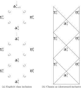
The result is the hierarchy shown in Figure 1.1. For more details, see [Kec95, Chapter 2, “Borel Sets”].

Theorem 1.3 ([And01, Exercise 3.9]). The Borel hierarchy when defined on a Polish space is proper untilΣ

e

0 ω1=Π

e

0 ω1 =∆

e

0 ω1.

We call the union of the countable levels of the hierarchy, , S

α<ω1∆_e

0 1, the

“Borel sets”, and denote the class of all such sets (for a given topological space

X) by BorelX. Since we are mostly concerned with the Baire space, we write

“Borel” for Borelω_ω.

An alternative, purely syntactic, characterisation of this hierarchy will also be useful. The account given here is simplified as much as possible for our present purposes; for more details, see [Kan03, pg. 152, “The Definability Con-text”].

Definition 1.4 (Second-order arithmetic). Second-order arithmetic

is the two-sorted structure

A2def=hω,ωω,ap,+,×,≤,0,1i

where ap : ω_{ω×ω→ω(function application) is defined by ap(a, n)}def

=a(n), and the other elements have their usual arithmetical definitions. The language has symbols for these elements, function variables ai ranging over ωω and number

variablesxiranging overω, and corresponding function and number quantifiers

∃1_,∀1 _{for elements of} ω_{ω and∃,∀for elements ofω.}

Terms for numbers are defined in the obvious manner, and if ϑ is a num-ber term and Φ a formula, the bounded quantifiers ∃xi<ϑΦ and∀xi<ϑΦ

∆ e 0 α+1 ⊆ ⊇ .. . Σ e 0 α ⊇ Π e 0 α ⊆ ∆ e 0 α .. . ∆ e 0 3 ⊆ ⊇ Σ e 0 2 ⊇ Π e 0 2 ⊆ ∆ e 0 2 ⊆ ⊇ Σ e 0 1 ⊇ Π e 0 1 ⊆ ∆ e 0 1

(a) Explicit class inclusion

? ? ? ? ? ? ? ? ? ? ? ? ? ? ? ? ? ? ? ? ? ? ? ? ? ÄÄÄÄ ÄÄÄÄ ÄÄÄÄ ÄÄÄÄ ÄÄÄÄ ÄÄÄÄ Ä ? ? ? ? ? ? ? ? ? ? ? ? ? ? ? ? ? ? ? ? ? ? ? ? ? _Ä Ä Ä Ä Ä Ä Ä Ä Ä Ä Ä Ä Ä Ä Ä Ä Ä Ä Ä Ä Ä Ä Ä Ä Ä ?? ?? ?? ?? ?? ?? ?? ?? ?? ?? ?? ??_? Ä Ä Ä Ä Ä Ä Ä Ä Ä Ä Ä Ä Ä Ä Ä Ä Ä Ä Ä Ä Ä Ä Ä Ä Ä ∆ e 0 1 ∆ e 0 2 ∆ e 0 3 Σ e 0 1 Σ e 0 2 Σ e 0 3 Π e 0 1 Π e 0 2 Π e 0 2

(b) Classes as (downward-inclusive) regions

Figure 1.1: Two visualisations of the Borel hierarchy

A hierarchy of formulae for second-order arithmetic analogous to the finite levels of the Borel hierarchy is defined as follows:

Definition 1.5 (Alternating quantifier hierarchy). Let Φ be a formula of second-order arithmetic containing only number quantifiers. Then

Φ∈Π0⇐⇒Φ∈Σ0

def

⇐⇒ the only quantifiers appearing in Φ are bounded,

Φ∈Σn+1

def

⇐⇒Φ is of the form∃xiΨ where Ψ∈Πn,

Φ∈Πn+1

def

⇐⇒Φ is of the form∀xiΨ where Ψ∈Σn.

By various quantifier rearrangement and coding equivalences (a prenex nor-mal form theorem for second-order logic), every formula of second-order arith-metic using only number quantifiers is equivalent to a formula in this hierarchy. Finally, the hierarchy is related to the Borel hierarchy of sets of reals by the following theorem:

Theorem 1.6 ([Kan03, Proposition 12.6]). Take A⊆ ω_{ω arbitrary. Then}

A∈Σ

e

0

and some b ∈ ω_{ω, we have a ∈ A ⇐⇒ Φ(a, b). Likewise for A ∈ Π}

e

0 n, with

Φ∈Πn.

This theorem means that we can place upper bounds on a set’s location in the Borel hierarchy simply by giving a defining formula for it.

1.2

The strength of determinacy axioms

Recall that forA⊆ ω_{X, G}

X(A) is the game where players play ωmoves

alter-nately fromX, and Iwins if the result lies in A. Recall also that a game is determined if a winning strategy exists for one of the players.

For Γ⊆

℘

X(Γ) is the statement “For

allA∈Γ, GX(A) is determined.” (As usual, we omit the subscript wherever

un-ambiguous.) Determinacy axioms can be used to show that the Borel hierarchy is in fact measuring complexity in some natural manner.

Theorem 1.7 ([Mar75]).

ZFC`Detω(Borel)

According to this theorem, the entire Borel hierarchy is determined. However [Fri81] showed that proving this requires uncountably many iterations of the power set operation.1 _{Less powerful axiom systems thanZFCprove determinacy}

less far up the Borel hierarchy, showing that topological complexity corresponds in some natural fashion to proof-theoretic strength.2

The idea is to start with a weak base theory T and measure the proof-theoretic strength of the systemsT+Det(Γ), for various Γ in the Borel hierarchy. More details can be found in [HMar], here only the flavour of the results is given.

The following results can be found in Chapter 1 of [Mar]:

Theorem 1.8 (Martin). Let ZFC− be the axiom systemZFCwithout the pow-erset axiom.

ZFC−`Det(∆

e

0

4) (Corollary 1.4.12)

ZFC−0Det(Σ

e

0

4) (Exercise 1.4.1)

[HMar] discusses further results based on weakenings ofSOA, an axiomati-sation of the system of second-order arithmetic. By the second result of Theo-rem 1.8,SOA0Det(Σ

e

0

4). HoweverSOAprovesDet(Σ

e

0

3) [HMar, via a theorem of

1

This statement is difficult to make precise without a lot of extra definitions; indeed, an earlier draft of this thesis attempted to do so and merely misrepresented the result. Broadly speaking, Friedman starts with the axiomatisation SOA _{of second-order arithmetic, and shows that} SOA+Detω(Borel) proves the existence of (codes for) every countable ordinal. HoweverSOA alone is not this powerful, so the extra proof-theoretic strength is the result of the determinacy axiom.

2

Welch]. Even weaker systems can be constructed by limiting the comprehension scheme and induction axiom (by restricting the formulae appearing within them to low levels of the alternating quantifier hierarchy). Some of these correspond exactly to lower-level determinacy axioms, however precise statements of these results would take us too far from the main ideas of the thesis.

The crucial point is that proofs of determinacy become more complicated for higher Borel levels, and (as the results above by Friedman and Martin show) this is by necessity. The games we are concerned with, however, lie in the lowest Borel levels. We can not only prove directly that they are determined, we can even construct winning strategies witnessing this.

1.3

Labellings

The classic determinacy proof is Gale and Stewart’s proof of open determinacy, Det(Σ

e

0

1). The technique of labelling used for this proof is the inspiration for all

the solution procedures presented here.

Definition 1.9 (Labellings). The classes

LI

def

={Iα;α∈Ord},

LD

def

={Dα;α∈Ord},

LII

def

={IIα;α∈Ord}

are called respectively theI-labels,D-labels andII-labels.

A labelling on a graphhV, Eiis a function

`: V →LI∪LD∪LII.

The set ran(`)∩LI is known as the I-labels of `, and likewise for D (the

draw labels) andII.

If`(v) =xα(forx∈ {I,D,II}), thenvis a vertex of heightα, and we say

ht`(v) =α.

We define two well-orders on labels,<I and<II, given by

Iα<I_,II Iβ

def

⇐⇒Dα<I_,IIDβ

def

⇐⇒IIα<I_,IIIIβ

def

⇐⇒α < β

and for allα, β, γ∈Ord,

Iα<IDβ<IIIγ, IIα<II Dβ<IIIγ.

The well-orders<I and<IIare in a sense preferences: each player prefers to

Definition 1.10 (Good strategies and sound labellings). LetG=hT,Ωi

be a game, and`: T →LI∪LD∪LII a labelling onT.

A strategyσfor playeri inGis`-good if for all positions s∈σowned by

iand labelled by`,

`(σ(s)) = min

<i

{`(sa<sub>x) ;x∈X} (or`(σ(s)) is undefined), and</sub>

σ(s) = min{sa_{x;x∈X and`(σ(s)) =`(s}a_x)}.

(We implicitly assume a suitable well-order on the move setX. Recall that the move set is finite, thus such an order always exists; for games on the Baire and Cantor spaces we use the usual ordering onω.)

The labelling ` isG-sound if every `-good strategyσ for playeri satisfies the following two conditions:

• σis winning for playerifrom positions labelled from Li;

• σis non-losing but not winning for playerifrom positions labelledDand owned byi.

Remark. These definitions are adapted from [LS05] but include a significant alteration: a labelling is not required to be total. Thus trivial (empty)G-sound labellings exist for any gameG. The advantage of this notation is that we can speak precisely about the process ofproducing a G-sound total labelling`, for instance by constructing a sequence of partial labellingsh`α;α < βisuch that

each`α is G-sound and ` = S{`α ; α < β} is both total and G-sound. The

following section provides an example of such a construction.

1.4

The Gale-Stewart labelling

The Gale-Stewart procedure was introduced in [GS53] to proveDet(Σ

e

0 1), that

open sets produce determined games. This procedure is the jump-off point for most of the algorithms considered in this thesis.

The idea will be familiar to game theorists, under the namebackward

in-duction. This idea in game theory has however become somewhat problematic,

since it depends on notions of rationality and rational play that turn out on closer inspection to be non-trivial.3 _{In the set-theoretic context these problems}

are avoided by strengthening the requirements on strategies: the properties we are interested in (being “winning” or “non-losing”) are required to hold against

any play by the other player.4

Informally, we start with the positions generating the basic open sets (at which we know the outcome), and then ‘back up’ the values through the tree by observing whereIcan move to aI-labelled node, and whereIIis forced to do so.

3

See for instance [dB04].

4

Definition 1.11. Let`be a labelling onT ⊆ <ω_{X. Letα} I

def

= sup{β+ 1 ;Iβ∈

ran(`)}, and similarlyαII and αD. Define the backup of `, backup(`)⊇` as

follows:

backup(`)(s) = 

             

             

`(s) ifs∈dom(`),

Iα_I if lh(s) even and`(t)∈LI for somet∈succ<sub>T</sub>(s), Iα<sub>I</sub> if lh(s) odd and`(t)∈LI for allt∈succ_T(s), IIα_II if lh(s) odd and`(t)∈LII for somet∈succ<sub>T</sub>(s), IIα<sub>II</sub> if lh(s) even and`(t)∈LII for allt∈succ_T(s), Dα_D if succT(s)⊆ran(`),{t∈succT(s) ;`(t)∈LD} 6=∅,

and{t∈succT(s) ;`(t)∈LI}=∅if lh(s) even,

{t∈succT(s) ;`(t)∈LII}=∅if lh(s) odd.

Theorem 1.12. Let G=hT,Ωibe a game,`a labelling onT. If`isG-sound, then so isbackup(`).

Proof. A backup(`)-good strategy is necessarily `-good, so we need only check the newly labelled positions.

Let σ be a backup(`)-good strategy, and s ∈ σ a position such that s ∈

dom(backup(`))\dom(`).

Suppose that backup(`)(s) ∈LI (the case forII is symmetric). If lh(s) is

even, then by construction `(σ(s)) ∈ LI, so by hypothesis σ is winning from

σ(s) (sinceσ is`-good), therefore σ is winning froms. If, on the other hand, lh(s) is odd, then by construction every sa<sub>x ∈ T must be labelled Iby `, so</sub>

again by hypothesisσis winning from every successor ofssoσis winning from

s.

Suppose instead that backup(`)(s)∈LD. By construction, if sis owned by

playerithen no successor ofsis labelled from Liby`, and all successors ofsare

labelled. Sinceσis`-good, no winning strategy forifromsexists. Furthermore, sinceσis backup(`)-good, a successor labelledD by` will be chosen. Finally, since` isG-sound, this successor is not winning for the opponent, soσ is non-losing forifroms.

Thus backup(`) isG-sound if`is. q.e.d

Definition 1.13. TheGale-Stewart labelling procedurelabels a tree

T ⊆ <ω_{X from a seed B⊆} <ω_{X as follows:}

`0(s) =

(

I0 if∃n∈ω(s¹n∈B),

⊥ otherwise. `α+1= backup(`α),

`λ=

[

{`α;α < λ}forλlimit.

Let γ be the least fixpoint of this procedure, then the total labelling `GS is

defined by

`GS(s) =

(

Lemma 1.14. The fixpoint γ exists.

[ Any stage that does not label a previously unlabelled position is the fixpoint. There are only countably many positions to label. ]

Theorem 1.15. Let A⊆ ω_{X be an open set with basis B. The Gale-Stewart} labelling`GS with seed B isG(A)-sound.

Proof. First, the labelling `0 is G(A)-sound. Let a ∈ <ωX be arbitrary such

that for somen ∈ ω, `0(a¹n) = I0. Then for some s ∈ B, s ⊆ a, so since B

is a basis for A, a ∈ A. That is, for any position s labelled I0 by `0, I has already won any play passing throughs, so all strategies (and thus all`0-good

strategies) are winning forIats.

Next, Theorem 1.12 guarantees that all successor-level labellings are G(A )-sound, so long as limit-level labellings are. So letλ∈ Ord be limit such that for all α < λ, `α is G(A)-sound. Any position s labelled such that `λ(s) ∈

LI received the label at some previous stage, say α. But by the inductive

hypothesis,`α was G(A)-sound, that is, any`α-good strategy is winning for I

ats. And if a strategyσis`λ-good, then it is also`α-good for allα < λ.

That is, both successor and limit stage labellings are G(A)-sound, so we need only check soundness of theII-labels of`GS.

Let T be the tree generated from A (i.e., T def= {a¹n ;a ∈A, n∈ω}). Let

σ be an `GS-good strategy for II in G(A) (so that σ ⊆ T), and let s ∈σ be

arbitrary such that`GS(s) =II0.

Assume toward a contradiction that for somea∈[σ] such thats⊆a,a∈A

(that is,σis not winning fromsforII).

Then since B is a basis for A, for some t∈B we have t⊆a. It cannot be thatt⊆s, since then`0(s) =I0, so we haves(t.

Now we show, towards a contradiction, that at some stageα < γ,`α(s) =Iα.

The proof is by induction alongt\s, showing that eacht(n) for n≥lh(s)−1 is labelledIat some stage beforeγ. The positiontprovides a base case.

For the inductive step, let u∈ σ be arbitrary such that for some α < γ,

`α(u)∈LI. Letv=u¹(lh(u)−1) be the predecessor ofu.

Supposevis owned byI. Then`α+1(v)∈LI. Suppose instead thatvis owned

by II. Then since σ is `GS-good, for all successors w ∈ succT(v), `γ(w) ∈ LI

(otherwise for somew∈succT(v),`GS(w)∈LII so σchooses w instead of u).

Letβ= sup{α;w∈succT(v), `γ(w) =Iα)}. Then ifβis limit,`β+1(v) =Iβ+1,

otherwise`β(v) =Iβ. This completes the inductive step.

By this induction, for no t ∈ σ such that t ⊇ s can it be the case that

`GS(t) ∈ LI while `GS(s) ∈ LII. So σ is winning for II from all II-labelled

positions.

We already showed that σ is winning for I from all positions labelled at successor and limit stages. So we have that σ is winning for player i from positions labelled i. Since σ was arbitrary `GS-good, this proves that `GS is

G(A)-sound. q.e.d

that such a strategy (for I) from a position labelled I moves always to a I -position labelled in a preceding stage. Since the ordinals are well-founded, a play according to such a strategy eventually passes through a position labelled

I0, confirming a win. For IIit suffices to avoid forever positions labelledI, in much the same way as the proof given above.

The more general construction via backup and soundness of labellings is given here because these building blocks will be reused in later sections.

1.5

Combinatorial labellings

Combinatorial labellings are introduced in [LS05]. The idea is to specify those labellings that are both sound (for their respective games) and are derived ‘bottom-up’ from the structure of the tree.

Definition 1.16 (Bisimulation). LethU, Ei and hV, Fi be directed graphs. A relationR⊆U×V is a bisimulation if the following two conditions hold:

∀u, u0∈U∀v∈V(ifuEu0 anduRv, then for some v0 ∈V,vF v0 andu0Rv0),

∀u∈U∀v, v0∈V(ifuRv andvF v0, then for some u0∈U,uEu0 andu0Rv0).

This is made clearer by a diagram, in which the dotted arrows are required by the definition:

u

E

²

²

R

/

/v

F

²

²

u

E

²

²

R

/

/v

F

²

²

u0 R _//v0 _u0 R _//v0

If we treat the graphs as transition systems thenRis a relation under which either system can simulate the other.

Definition 1.17. LetT⊆ <ω_{X a tree andA⊆} ω_{Xbe arbitrary, andR⊆T×T}

a bisimulation on the positions inT. We sayRpreservesAif for alla, b∈[T] we have

if∀n∈ω(ha¹n, b¹ni ∈R) thena∈A⇐⇒b∈A.

We extend this to a gamehT,Ωiby requiring thatR preserve ΩI, ΩD and

ΩII, and say thatRpreserves Ω.

If s, t ∈ T are positions both owned by the same player, we say they are Ω-bisimilar if there exists an Ω-preserving bisimulationRsuch thatsRt.

A combinatorial (‘bottom-up’) labelling should respect bisimulation. Intu-itively, if two positions are bisimilar then the trees below them ‘look the same’ from the point of view of playing the game. A bottom-up labelling should thus not distinguish between them.

Definition 1.18. A labelling`for the treeT is Ω-combinatorialif for every

Theorem 1.19 ([LS05, Proposition 4.2]). There is a Σ

e

0

2 set A⊆ ω2 such

that noG(A)-sound labelling is A-combinatorial. Proof. Define Aby

a∈A⇐⇒ ∃def n∈ω∀m≥n(a(m) = 0).

ClearlyAisΣ

e

0

2, andIIhas many winning strategies (“move always 1” is a very

simple one). But by observation, any twos, s0 _∈ ω_{2 owned by the same player}

areA-bisimilar. (Take the bisimulation{­

sa_{t, s}0a_t®_;t∈ ω_{2} as witness.) This}

means that anyA-combinatorial labelling` must give every position with odd length the same label. And in that case, a strategy forII that is `-good will

makeIIalways move 0. q.e.d

In fact, [LS05] shows thatΣ

e

0

2 is the first Borel class containing a game that

does not admit a combinatorial labelling:

Theorem 1.20 ([LS05, Theorem 6.5]). Every ∆

e

0

2 set A has a totalG(A) -sound andA-combinatorial labelling.

Proof sketch. The proof proceeds by constructing G(A)-sound andA-combinatorial labellings for setsAin the Hausdorff difference hierarchy. By a theorem of Haus-dorff and Kuratowski,∆

e

0

1is the union of all countable-level Hausdorff difference

classes. q.e.d

1.6

The combinatorial game

Definition 1.21. The combinatorial game on a tree T ⊆ <ω_{X is the}

rulification of the gamehT,Ωiwhere ΩD= [T].

That is, plays within the tree are a draw, otherwise the first player to exit the tree loses. (Note that this is therefore a game G(A, B) with A, B ⊆ ω_X

both open.)

The obvious extension of the Gale-Stewart procedure suffices to label a tree for solving the combinatorial game.

Definition 1.22. Thecombinatorial Gale-Stewart procedure labels a treeT ⊆ <ω_{X according to two seedsB, C ⊆} <ω_{X as follows:}

`0(s) =



 

 

I0 if∃n∈ω(s¹n∈B),

II0 if∃n∈ω(s¹n∈C),

⊥ otherwise. `α+1= backup(`α),

`λ=

[

{`α;α < λ}forλlimit.

Letγ be the fixpoint of this procedure, then the total labelling`CGS is defined

by

`CGS(s) =

(

Remark. This definition can only be applied ifB and C are ‘strongly disjoint’ in the following sense: ∀s∈B∀t∈C(¬(s⊆t∨t⊆s)). This condition is obviously satisfied by the seeds produced by the combinatorial game, which is all we need for the present purposes.

Theorem 1.23. LetG(A, B)be a combinatorial game, the rulification of a tree

T ⊆ <ω_{X, and let C, D ⊆} <ω_{X be bases for A and B, respectively. Then the} combinatorial Gale-Stewart labelling`CGSwith seedsCandDisG(A, B)-sound. Proof. The proof for positions labelled IandIIis analagous to that for Theo-rem 1.15.

Lets∈ <ω_{X be a position such that`}

CGS(s) =D0, and letγbe the fixpoint

of the sequence of backup labellings. Without loss of generality, let lh(s) be even (the proof for positions owned byIIis analagous). It suffices to show two things: no successor ofsis labelledI, and some successor ofsis labelledD.

(These two requirements ensure that an`CGS-good strategy forIis drawing,

while the absence of a winning strategy is shown by the same argument as demonstrated the soundness of aII-label given by`GS: if such a strategy existed,

swould be labelledIbefore`γ.)

But the two requirements follow directly from the definition of backup: since

sis owned byI, if some successortbecomes labelledIat stageα, then`α+1(s) = I. Likewise, if all successors are labelled II at stages before γ, then `γ(s) =

II. q.e.d

However there is another labelling procedure that also suffices. Again, the definition is given here mainly so we may make use of variations on this idea in later chapters.5

Definition 1.24. The two-pass labelling `twice for a combinatorial game

G(A, B) on <ω_{X is given by the following definition: first, letB}0_={h0ia_s;s∈

B}. Now take`A=`GSapplied to G(A), and`B0 =`GS applied to G(B0)

`twice(s)

def

= 

 

 

`A(s) if`A(s)∈LI, IIα if`B(h0ias) =Iα, D0 otherwise.

In essence, we analyse the two open games given by A and B to get the positions winning forIand II, and any position lying in the closed portion of both these games is drawing.

Theorem 1.25. For any combinatorial game G(A, B), the two-pass labelling

`twice isG(A, B)-sound.

Proof. Let σbe an `twice-good strategy. Clearly, σ is also`A-good. Lets∈σ

be labelledI. Then since`Ais G(A)-sound, [σ]∩[s]∈A.

5

Suppose instead that `twice(s) ∈ LII. Then let σ0 = {h0iat ; t ∈ s} be a

strategy forIin G(B0). Clearly,σ0 is`B0-good, and`_B0 is G(B0)-sound. Since

`B0(h0ias)∈LI, σ0∩[h0ias]∈B0. But then by construction, [σ]∩[s]∈B.

Finally, takes∈σsuch that`twice(s) =D0. This means that both `A(s) = II, and`B0(s) =II.

Since againσis G(A)-good, we have [σ]∩[s]⊆ ω_X\A.

Since`B0(h0ias) =II, [σ0]∩[h0ias]⊆ ωX\B0, that is, [σ]∩s⊆ ωX\B.

Putting these two together gives us [σ]∩[s]⊆ ω_{X\(A∪B), that is,σis a}

drawing strategy.

All that remains is to show that no winning strategy from s exists when

`twice(s) = D0. Now suppose without loss of generality that lh(s) is even (the

case for positions owned byIIis analagous, but complicated by the extra first move, so we shall omit it). Note that a winning strategy forIin G(A, B) also wins G(A). Butσis`A-good, and`A(s) =II, so no winning strategy forIfrom

Chapter 2

Automata games

In this chapter I consider a number of classes of games played on finite graphs, taken from the automata theory literature. These games allow for a new com-plexity analysis, roughly speaking “How difficult is it to play according to a given strategy?” Specifically, how much extra information beyond the structure of the graph does the player need to remember, in order to play according to a given strategy?

2.1

Definitions

An automaton is essentially a graph with the edges labelled. Conceptually, the vertices of the graph represent configurations of a machine, and an labelled edge represents a change from one configuration (or state) to another, driven by the input of the machine.

Definition 2.1 (Automata). An automaton Aover a finite alphabet Σ is a structurehQ, q0, δiwhereQ={q0, q1, . . . , qn} is a finite set of states,q0 is

thestart state, andδ:Q×Σ→Qis the transition function.

The graph ofAishQ, EiwhereE⊆Q×Qis given by

hq, q0i ∈E⇐⇒ ∃def a∈Σ(δ(q, a) =q0).

We represent an automaton pictorially by drawing its graph and labelling the edges with the appropriate inputs to the transition function. Figure 2.1 shows a simple example.

Let A = hQ, q0, δi be an arbitrary automaton. Intuitively the automaton

notion represents a machine with moving parts, which changes its configuration from state to state in response to input.

The response of A to a nonempty sequence (response_A: <ω_{Σ → Q) is}

defined inductively as follows:

responseA(hxi) =δ(q0, x),

?>=<

89:;

0

*

*

_?>=<

_89:;

1 0

j

j

1

/

/

?>=<

89:;

Figure 2.1: An automaton hQ, q0, δi with state set {q0, q1, q2} and transition

function©

hq0,0, q1i,hq1,0, q0i,hq1,1, q2i

ª .

Thetrace of a (possibly infinite) sequences∈ ≤ω_{Σ is given by}

traceA(s) =hresponseA(s¹n) ; 0< n≤lh(s)i.

In both cases we omit the subscript wherever unambiguous. We also say response(s) = trace(s) = ⊥ if δ is undefined on some necessary input for the induction.

Definition 2.2 (Languages). A language L over a finite alphabet Σ is a set of finite sequences with elements from Σ, i.e.,L⊆ <ω_{Σ. An ω-language}

is a set ofinfinitesequencesLω⊆ ωΣ, and its elements are known asω-words.

An automatonA accepts a finite sequencesif traceA(s)6=⊥.

Anω-automatonis a pairhA,ΩiwhereAis an automaton with state set

Qand Ω⊆ ω_{Qis the acceptance condition. An ω-wordais accepted by}

anω-automaton hA,Ωiif for alln∈ω Aacceptsa¹n, and if trace(a)∈Ω. We call the set of finite sequences accepted by an automaton A the

lan-guage generated by A, and the ω-words accepted by hA,Ωi the ω-

lan-guage generated byhA,Ωi, denoted by L(A,Ω).

2.2

Standard acceptance conditions

In this section I give some standard acceptance conditions that can be defined in a natural way on the graph of the automaton, and show their complexity with respect to the Borel hierarchy. All conditions are given with respect to an automatonA=hQ, q0, δi.

2.2.1

Reachability

LetQT⊆Qbe thetarget set. The acceptance condition ΩRis the set of all

(infinite) traces that pass though an element ofQT:

Definition 2.3.

ΩR

def

={a∈ ωQ;∃n∈ω(a(n)∈QT)}.

Theorem 2.4. For all reachability condition ω-automatahA,ΩRi,L(A,ΩR)∈ Σ

e

0

1. Furthermore, there exists such an automaton withL(A,ΩR)6∈∆

e

0

1.

Proof. The basis of finite sequences whose last element is inQTgenerates ΩR.

For the second statement, letAbe given by

?>=<

89:;

3

3

1

/

/

89:;

?>=<

k

withQT={q1}. LetL=L(A,ΩR) for brevity. IfLis closed, then for some tree

T ⊆ <ω_{2,L= [T]. For eachn∈ω,h0}n₁ω_{i ∈ L. Since T is closed under initial}

subsequence, this means that for alln∈ω,h0n_{i ∈T. But thenh0}ω_{i ∈[T], and}

h0ω_{i 6∈ L. Thus no suchT exists. q.e.d}

2.2.2

The B¨

uchi condition

LetQTbe the target set. The acceptance condition ΩB is the set of all infinite

traces that passinfinitely often through an element ofQT. Definition 2.5.

ΩB

def

={a∈ ω_{Q;∀n∈ω∃m>n(a(m)∈Q}

T)}.

Theorem 2.6. For all B¨uchi condition automata hA,ΩBi, L(A,ΩB) ∈ Π

e

0 2. Furthermore, there exists such an automaton withL(A,ΩB)6∈Σ

e

0 2.

Proof. That L(A,ΩB) ∈ Π

e

0

2 for any B¨uchi automaton can be seen from an

alternating quantifiers argument. The two quantifiers in the defining formula bound the depth to which the trace has to be evaluated, and checking the membership inQTobviously only requires bounded quantifiers.

For the second statement, take the very simple automaton with alphabet

{0,1}given by the picture

?>=<

89:;

1

*

*

0

3

3 jj ₀

?>=<

89:;

and letQT ={q1}. Let L=L(A,ΩB). Suppose towards a contradiction that

L ∈ Σ

e

0

2. Then for some sequence hAn ∈ Π

e

0

1 ; n < ωi,

S

{An ; n ∈ ω} = L.

Now we use a diagonalisation argument to construct an elementathat does not appear inS_{

An;n∈ω}, but such thata∈ L.

First note that each An = [Tn], for suitable trees Tn ⊆ <ω2. We will find

an increasing family of sequences hsn ∈ <ωX ; n ∈ ωi such that for each n,

sn ( sn+1 but also for each n, sn 6∈ Tn. This guarantees that a = S{sn ;

n ∈ ω} 6∈ S_{

An ; n ∈ ω}, however at the same time we will ensure that

trace(a)∈ΩB.

Let m0 ∈ ω be least such that h0m0i 6∈ T0. Such an m0 exists, otherwise

h0ω_{i ∈ [T}

n] and the trace through this sequence visits q1 only finitely many

times. Since Tn is a tree, closed under initial subsequence, h0m1i 6∈ Tn. Let

s0=h0m1i.

Now for the inductive step: let mn+1 ∈ω be least such thatsnah0mn+1i 6∈

Tn+1. Again, such anmn+1 exists, because otherwisesnah0ωi ∈[T]. Then set

sn+1=snah0mn+11i.

Finally, take a = S

{sn ; n ∈ ω}. Since for each n, sn+1 ) sn, we have

a∈ ω_{2. In addition, since eachs}

n ends with a 1,q1 is visited infinitely often in

trace(a). But thena∈ L, while the construction ensures that

This contradiction shows that such a sequence of closed sets such that S

hAni=L(A,ΩB) cannot be found. That is, for this automaton,L(A,ΩB)6∈ Σ

e

0

2. q.e.d

2.2.3

The Muller condition

LetQT ⊆

℘

requires that an accepted trace visit all and only the elements of some target set infinitely often.

Definition 2.7. Leta∈ ω_{Xbe an arbitrary infinite sequence. The set Fin(a)⊆}

Xcollects all elements fromaoccurring only finitely many times, while Inf(a)⊆

X collects those elements occurring infinitely many times.

Inf(a)def

={x∈X;∀n∈ω∃m>n(a(m) =x)},

Fin(a)def={x∈X;∃n∈ω∀m>n(a(m)6=x)}.

Definition 2.8.

ΩM

def

={a∈ ω_{Q;∃P ∈Q}

T(Inf(a) =P)}.

Theorem 2.9. For all Muller conditionω-automatahA,ΩMi,L(A,ΩM)∈∆

e

0

3.

Furthermore, there exists such an automaton withL(A,ΩM)6∈Σ

e

0

2∪Π

e

0

2.

Proof. Suppose first thatQT={S}is a singleton.

ForA⊆Q, Let Φ(a, A) represent the formula

∃n∈ω∀m>n(response(a¹m)∈A).

Then Φ(a, S) is a Σ

e

0

2 formula specifying that Inf(trace(a)) ⊆ S. As before,

taking traces and testing membership in S can be done using only bounded quantifiers.1

Then for each A(S,¬Φ(a, A) isΠ

e

0 2. And

Φ(a, S)∧ ^

A(S

¬Φ(a, A)

is a∆

e

0

3formula specifying precisely thata∈ΩM. In caseQTis not a singleton,

we have only a finite disjunction of such formulae, so the result is still∆

e

0

3.

To see that Σ

e

0

2 does not suffice, we can take the construction given in the

proof of Theorem 2.6 (the Borel height of B¨uchi conditions). If we take a singleton condition ΩΣwith target setsQΣ

def

={{q0, q1}}, exactly the same

con-struction shows that anyΣ

e

0

2 set either misses an elementathat we want (with

Inf(trace(a)) = {q0, q1}) or includes one we don’t want (with Inf(trace(a)) =

{q0}).

1

To see that Π

e

0

2 does not suffice, take the same automaton but with the

Muller condition ΩΠ given by the target setsQΠ

def

={{q1}}. If this isΠ

e

0 2, then

its negation isΣ

e

0

2. But the negation of this condition states precisely thatq0

appears infinitely often in trace(a), the B¨uchi condition{q0}, and we showed

above that this is notΣ

e

0

2.

So we have two Muller conditions, one not in Σ

e

0

2 and one not inΠ

e

0 2. But

we can combine them into a single automaton, in the following simple manner, as in the following picture.

?>=<

89:;

1

*

*

0

)

)

?>=<

89:;

j

j _kk 1

?>=<

89:;

0 > > } } } } } } } } } 1 Ã Ã A A A A A A A A A

?>=<

89:;

1

*

*

0

K

K

?>=<

89:;

q4 0

j

j _kk 1

The states of the two automata are renamed so that they are disjoint. The first transition of the new automaton selects which of the sub-automata to use. The Muller condition Ω∆ is defined from the union of the two sub-automata

conditions, target sets {{q1, q2},{q3}}. If this isΣ

e

0

2 or Π

e

0

2, then the relevant

condition can be extracted simply by looking at the first element of the trace:

trace(a)∈ΩΣ⇐⇒trace(a)∈Ω∆∧a(0) = 0,

trace(a)∈ΩΠ ⇐⇒trace(a)∈Ω∆∧a(0) = 1.

Since the test on the first element is quantifier-free, either of the two conditions can be reduced to this one without changing Borel classes. To avoid contradic-tion, Ω∆6∈Σ

e

0

2∪∆

e

0

2. q.e.d

2.2.4

Summary

The conditions considered have been chosen because they make a relatively neat and tidy hierarchy according to topological complexity. Figure 2.2 summarises the situation. (The positions shown are the highest extent of the relevant con-ditions, of course simple instances of complex conditions also exist.)

2.3

Automata games and strategies

? ? ? ? ? ? ? ? ? ? ? ? ? ? ? ? ? ? ? ? ? ? ? ? ? ÄÄÄÄ ÄÄÄÄ ÄÄÄÄ ÄÄÄÄ ÄÄÄÄ ÄÄÄÄ Ä ? ? ? ? ? ? ? ? ? ? ? ? ? ? ? ? ? ? ? ? ? ? ? ? ? _Ä Ä Ä Ä Ä Ä Ä Ä Ä Ä Ä Ä Ä Ä Ä Ä Ä Ä Ä Ä Ä Ä Ä Ä Ä ?? ?? ?? ?? ?? ?? ?? ?? ?? ?? ?? ??_? Ä Ä Ä Ä Ä Ä Ä Ä Ä Ä Ä Ä Ä Ä Ä Ä Ä Ä Ä Ä Ä Ä Ä Ä Ä ∆ e 0 1 ∆ e 0 2 ∆ e 0 3 Σ e 0 1 Σ e 0 2 Σ e 0 3 Π e 0 1 Π e 0 2 Π e 0 2 ΩR ΩB ΩM

Figure 2.2: Highest positions of automata conditions in the Borel hierarchy

about the state of the machine, not about the particular moves the environment plays. These notions are formalised as follows:

Definition 2.10 (Automata games). An alternating automatonis an structure

hQ, q0, QI, QII, δi

where hQ, q0, δi is an automaton, such thatQI and QII partition Q, q0 ∈QI,

and for allx∈Σ, ifq∈QIthen δ(q, x)∈QII, and ifq∈QII thenδ(q, x)∈QI

(where these are defined).

Theautomaton gamefor an alternatingω-automatonhA,Ωiis the game

hT, AiwhereT ⊆ <ω_{Σ andA⊆[T] are given by}

s∈T ⇐⇒ Adef acceptss, a∈A⇐⇒def traceA(a)∈Ω.

Lemma 2.11. For any strategy σ ⊆ <ω_{Q on the tree of traces, a strategy}

τ⊆ <ω_{Σon the tree of moves exists such that{trace(t) ;t∈τ}=σ.}

Definition 2.12 (Automata strategies). Let A= hQ, q0, QI, QII, δi be an

arbitrary alternating automaton with alphabet Σ. Anautomaton strategy

for a game played onAis a structure

hM, m0, σi

where M is an arbitrary set known as the memory, containing at least one elementm0∈M, thestarting configuration, andσ:Q×M →Σ×M is

a function that both chooses a move and updates the memory. An automaton strategy forIis defined on all pairs inQI×M, and likewise forIIonQII×M.

We refer to the strategy as a whole as “σ” where this will not cause confusion.

While the plays in an automaton game are just ω-words, to match them to automaton strategies we have to go via the states of the automaton.

Definition 2.13 (Plays according to σ). LetA=hQ, q0, QI, QII, δibe an

alternating automaton with alphabet Σ,hM, m0, σia strategy forI(the

alter-ations necessary for II are obvious). Let aII ∈ ωΣ be an arbitrary ω-word,

representing the moves byII.

The definition of the play constructed byσ is given inductively in terms of

aI ∈ ωΣ (the moves played by I, generated by σ), ~q ∈ ωQ (the states passed

through byA),m~ ∈ ω_{M (the memory states used byσ) andaII:}

~

q(0) =q0,

~

m(0) =m0,

Forn= 2k(moves byI):

haI(k), ~m(k+ 1)i=σ(~q(2k), ~m(k)),

~

q(2k+ 1) =δ(~q(2k), aI(k));

Forn= 2k+ 1 (moves by II):

~

q(2k+ 2) =δ(~q(2k+ 1), aII(k)).

This should be made clearer by a picture:

δ ~q σ aI m~ aII

q0 m0

σ(q0, m0) = ha0, m1i

δ(q0, a0) = q1 a1

δ(q1, a1) = q2 σ(q2, m1) = ha2, m2i

δ(q2, a2) = q3 a3

δ(q3, a3) = q4 σ(q4, m2) = ha4, m3i

δ(q4, a4) = q5 a5

..

Finally, we construct the resulting playa⊆ ω_{Σ as follows: fork∈ω,}

a(2k) =aI(k),

a(2k+ 1) =aII(k).

We call athe response ofσandAto aII. A playb∈ ωΣ is according

to σand Aif there is some c∈ ω_{Σ such thatb is the response of σandA to}

c. The sequence~qis the state response ofσandAtoaII, and such a state

sequence is also according to σandAif a suitablec∈ ω_{Σ exists.}

We need to update our definition of strategy equivalence: two strategies (automata or ordinary tree-form)σandτ are play equivalent if the plays according toσare exactly the plays according toτ.

The formal details of this definition are tiresome, but the idea is fairly sim-ple. An automaton strategy isolates the computational mechanism used to produce the next move, and the size of the memoryM provides a measure of the complexity of that mechanism. The terminology for automaton strategies is deliberately reminiscent of that for ordinary tree-form strategies. The following two theorems justify this notational overloading.

Theorem 2.14. Letσbe an automaton strategy for the automaton gamehA,Ωi

with state setQ. Then there exists a strategyτ ⊆ <ω_{Qsuch thatq~∈[τ]iff~qis} a state sequence according toσandA.

In ordinary words: every automaton strategy can be transformed into an equivalent (up to traces) strategy on the trace tree.

Proof. Obvious, by an inductive construction taking partial responses of σ to

finite sequences. q.e.d

Theorem 2.15. Letσ⊆ <ω_{Qbe a strategy (on the trace tree) for an automaton} gamehhQ, q0, δi,Ωi. Then there exists an automaton strategy hM, m0, τi play equivalent toσ.

Proof. Take M = <ω_{Q, m}

0=hi, and defineτ as follows:

τ(q0,hi) =hσ(hi), δ(q0, σ(hi))i,

and fors6=hi,

τ(q, s) =­

σ(sa_{q), s}a_qa_{δ(q, σ(s}a_q))®

δ ~q τ aI m~ aII

q0 hi

τ(q0,hi) = ha0, hq1ii

δ(q0, a0) = q1 a1

δ(q1, a1) = q2 τ(q2,hq1i) = ha2, hq1, q2, q3ii

δ(q2, a2) = q3 a3

δ(q3, a3) = q4 τ(q4,hq1, q2, q3i) = ha4, hq1, q2, q3, q4, q5ii

δ(q4, a4) = q5 a5

..

. ... ... ...

Clearly, the memory is tracking the play history. Since the move chosen byτ is simply the response ofσto that history, the response to anyaII is a branch of

σ. q.e.d

So we can freely transform back and forth between ordinary strategies (on traces) and automata strategies. But in the general case, the automaton strategy corresponding to a trace strategy requires infinite memory. We are particularly interested in cases where not all of the play history need be used to produce a winning strategy.

Definition 2.16. LethM, m0, σibe an automaton strategy. If|M|= 1, we call

σ memoryless. If|M|< ω,σis finite-memory.

Lemma 2.17. If the plays according to a function σ:Q →Σ are defined for each player in the obvious manner, then for every memoryless automaton strat-egy hM, m0, τi there exists a function ρ: Q → Σ which is play equivalent to

τ.

[ Obvious. ]

By an abuse of terminology we refer also to ρ in the above lemma as a memoryless strategy. Our first example of such a strategy is for the reachability game, however it will be useful to study instead a generalised version based on the combinatorial game.

2.3.1

The combinatorial automaton game

The combinatorial automaton game is a generalised form of the reachability game. The first player unable to move loses, while infinite plays are a draw. In fact we have already seen this game, in section 1.6: the combinatorial automaton game on an automatonA is simply the combinatorial game on the unravelled tree of the graph ofA.

Definition 2.18. If A = hQ, q0, QI, QII, δi is an alternating automaton, the

combinatorial automaton game onAis a pair

whereδ0 is given by

δ0(q, x) = 

 

 

δ(q, x) if this is defined, otherwise

⊥I ifq∈QI∪ {⊥I},

⊥II ifq∈QII∪ {⊥II}.

and Iwins traces containing ⊥II, IIwins traces containing ⊥I, and all other

traces are a draw.

Remark. The definition of the combinatorial automaton game cannot be given in the formalism we use for other automata games, because specifying only the winning set forIdoes not fully describe the payoffs. This is no great problem, since we will be using the game only to assist with various proofs, and these will rely on results shown on the combinatorial game on trees, for which we

do have a proper formal representation. Likewise, the derived automatonA0 _is not properly speaking an alternating automaton, since both players play from the states⊥I and ⊥II. This could easily be remedied, but at the cost of some

clarity. For similar reasons, we cannot strictly speaking place the combinatorial automaton game in the Borel hierarchy. However ‘morally speaking’ it is Σ

e

0

1,

since the sets of winning plays for both players are open.

Theorem 2.19. For every reachability gamehA=hQ, q0, QI, QII, δi,ΩRi gen-erated by QT ⊆Q, there exists a combinatorial automaton game on an alter-nating automatonB with the same set of winning traces.

Proof. Form the new alternating automatonBby making the following changes to A: remove all transitionshq, x, pi ∈ δ where q∈QT. Add a new stateq⊥, and transitionsδ(q, x) =q⊥for allx∈X andq∈QI∩QT. Also add the system

GFED

@ABC

0,1

+

+

_GFED

_@ABC

β 0,1

k

k

and for every x∈ X, for each q ∈ QI\QT a transitionδ(q, x) = qα, and for

eachq∈QII\QT, a transitionδ(q, x) =qβ .

This last step ensures thatIInever wins the combinatorial automaton game (Ialways has an option to draw). And a play wins forIonly if it passes through an element ofQT, since these are the only leaves in the graph ofB. q.e.d

2.4

Memory requirement as complexity

The results in this section show how the memory requirements for automata strategies compare to the set-theoretic complexity analysis in terms of the payoff set.

Theorem 2.20. Memoryless strategies suffice for combinatorial graph games. That is, if a winning (resp. non-losing) strategy exists for a combinatorial game

Proof. Recall that the combinatorial Gale-Stewart labelling`CGS(Definition 1.22)

is G(A, B)-sound whereAandBare open (specifically, where G(A, B) is a com-binatorial game, the rulification of a tree). The proof proceeds by defining a similar labelling on the graph (which produces a memoryless automaton strat-egy), and showing that the unravelling of the labelled graph is the labelled tree. Since the tree labelling is G(A, B)-sound, so is the graph labelling.

Definition 2.21. The combinatorial graph labelling procedure la-bels the graph G = hQ, Ei of an alternating automaton hQ, q0, QI, QII, δi as

follows:

`0(q)

def

= 

 

 

I0 if succG(q) =∅∧q∈QII, II0 if succG(q) =∅∧q∈QI,

⊥ otherwise;

`n+1

def

= backup(`n);

`ω

def

=[{`n;n∈ω};

`CG(q)

def

= (

`ω(q) if this is defined, D0 otherwise.

Lemma 2.22. For somek∈ω,`k=`ω.

[ Each stage is either a fixpoint or labels one new vertex. There are only finitely many vertices to label. ]

Let`CGSbe the labelling produced by the combinatorial Gale-Stewart

proce-dure on the unravelled treeT ofG, with the seedsA={(sa_{q)∈T ; succ} G(q) =

∅∧lh(s) is even}, B ={(sa_{q)∈T ; succ}

G(q) =∅∧lh(s) is odd}. (We must

also addhitoB if succG(q0) =∅.)

Let`CGbe the labelling produced by the combinatorial graph labelling

pro-cedure onG.

Letσ:Q→X be an `CG-good memoryless strategy for playeri. Derive a

strategyτ on the trace tree by taking, fors∈ <ω_{Qowned byi,}

succτ(s) =©saσ(s(lh(s)−1))ª

(and succτ(hi) =hσ(q0)iifσis a strategy forI).

Lemma 2.23. The strategies σandτ are play-equivalent.

[ Obvious. ]

Lemma 2.24. The strategy τ isG(A, B)-sound.

Lemmas 2.23 and 2.24 together guarantee thatσis sound for the

combina-torial graph game, proving the theorem. q.e.d

Corollary 2.25. Memoryless strategies suffice for the reachability game. Remark. For the more complex automata games, we often stipulate that the graph of the automaton is pruned, so that only ‘true’ infinite plays need be considered. Theorem 2.20 in a sense justifies this decision: if the automaton is not pruned, we can augment the condition with a combinatorial automaton game, solve this to produce memoryless strategies for both players, and solve the original game restricted to the pruned graph whose vertices receiveDlabels in the combinatorial game.

Theorem 2.26. Memoryless strategies suffice for B¨uchi games.

Proof sketch. Let G=hQ, Eibe the graph of an automaton. Take the B¨uchi game fromq0∈Qwith target setQT⊆Q. As before, we will define a labelling

on the graph. The details of the correspondence to the trace tree are omitted. First, for eachq∈QTdefine a labelling`q for the reachability analysis with

target set{q}. Recall that the reachability game from q0 is not automatically

won ifq0 ∈ QT, so for each q ∈ QT such that `q(q) ∈ LI, Ican force a cycle

that includesq.

LetQC be the set of these ‘cyclable’ target states. Now use this as the seed

for another reachability analysis. Call the resulting labelling`B.

That`Bis sound also when lifted to the trace tree follows from the soundness

of reachability labellings. For anys∈ <ω_{QlabelledInwithn >0, the soundness}

of reachability labellings guarantees that everya∈[s] (restricted to an`B-good

strategy) passes through a position labelledI0. Likewise, for every such position, it is guaranteed that every branch passes through another such, and the B¨uchi winning condition is satisfied by an inductive argument.

Conversely, from a positionslabelledII, the branches throughsdo not pass through a vertex labelledI0. That this is sufficient forIIto win is a consequence of the choice ofQC; again by reachability, forq∈QT\QC, IIhas a strategy

that does not return to q. If `B(saq) ∈ LII, and if τ ⊆ <ωQ is an `B-good

strategy, then for alla∈[τ]∩[sa_{q], qdoes not recur ina, nor do any elements}

ofQC. Furthermore, since the same holds for allq∈QT\QC labelledII, and

since ifs⊆ais labelledIIthe same will hold for allt⊆a(sinceτ is`B-good),

no element ofQT occurs infinitely often ina. q.e.d

Theorem 2.27. Memoryless strategies do not suffice for Muller games. That is, there exists a Muller game for whichIhas a winning strategy but no winning memoryless strategy.

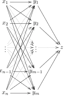
Proof. Take the automaton

?>=<

89:;

0

*

*

1

·

·

?>=<

89:;

j

j

?>=<

89:;

0,1

T

with the condition ΩM = {{q1, q2}}. It is clear that Ihas a winning strategy

(for instance, alternating playing 0 and 1) and equally clear that no winning

memoryless strategy exists. q.e.d

So far it seems that increasing memory requirements correspond to increasing topological complexity. Our first example of a game that does not always admit memoryless strategies is also the highest in the Borel hierarchy. However the correspondence is only apparent. To show this, we need to introduce one more automaton condition.

Definition 2.28. The parity condition is a function f: Q→ω assigning to each state a value. We lift f to traces in the obvious manner: tracef(s) =

hf(response(s¹n)) ;n≤lh(s)i. Player Iwins a play awith parity condition f

if the highest value occurring infinitely often in tracef(a) is even.

Theorem 2.29 ([Far02, Theorem 1.22]). The class ofω-languages accepted by parity automata is precisely those accepted by Muller automata.

This of course means that the topological complexity of these two conditions is the same.

Theorem 2.30 ([K¨us02]). Memoryless strategies suffice for parity condition games.

Theorems 2.29 and 2.30 demonstrate that the memory requirements com-plexity measure is sensitive to details of the games that do not affect the topol-ogy of the payoff sets. Less obviously, they place an upper bound on memory requirements for Muller games.

Theorem 2.31 ([Maz02, Theorem 2.7]). Finite memory suffices for Muller games.

Proof sketch. By Theorem 2.29, for every Muller condition automaton Athere is a parity condition automaton B that accepts the same ω-language. Sup-poseIhas a winning strategy for the game onB. By Theorem 2.30, he has a memoryless winning strategy, sayσ.

Now he can build a winning automaton strategy τ for A, using the states ofB for the memory. The memory traces a simulated path through B, and σ

generates his moves. Sinceσ is winning, the resulting play is accepted by B,

and therefore also byA. q.e.d

2.5

Summary