Local polynomial regression for circular predictors

promoting access to White Rose research papers

White Rose Research Online

[email protected]

Universities of Leeds, Sheffield and York

http://eprints.whiterose.ac.uk/

This is a final published version of a paper accepted for publication in Statistics

& Probability Letters.

White Rose Research Online URL for this paper:

http://eprints.whiterose.ac.uk/42948/

Paper:

Di Marzio, M, Panzera, A and Taylor, CC (2009)

Local polynomial regression for

circular predictors.

Statistics & Probability Letters, 79 (19). 2066 – 2075.

Local polynomial regression for circular predictors

Marco Di Marzioa_{, Agnese Panzera}a_{, Charles C. Taylor}b,1

a_{DMQTE, Universit`a di Chieti-Pescara, Viale Pindaro 42, 65127 Pescara, Italy.}

b_{Departement of Statistics, University of Leeds, Leeds LS2 9JT, UK.}

Abstract

We consider local smoothing of datasets where the design space is the d-dimensional (d≥1) torus and the response

variable is real-valued. Our purpose is to extend least squares local polynomial fitting to this situation. We give both theoretical and empirical results.

Key words: Circular data, circular kernels, von Mises weight function, weighted least squares. 2000 MSC: 62G07 - 62G08 - 62G20

1. Introduction

A circular observation can be regarded as a point on the unit circle, or a direction in the plane. Once an initial direction and an orientation of the unit circle have been chosen, any circular observation may be represented by an

angleθ∈ [0,2π). Typical examples include flight direction of birds from a point of release, wind and ocean current

direction, energy demand over a period of 24 hours when the measurements are taken over a time interval much longer

than the day and when the times of the day are recorded. A circular observation is periodic, i.e.,θ =_θ+_2mπfor

m∈Z. This periodicity sets apart circular statistical analysis from standard real-line methods. Recent accounts are

given by Jammalamadaka & SenGupta (2001) and Mardia & Jupp (1999).

A much less studied subject is local regression in the case of circular predictors and real-valued responses. Its practical relevance is easily seen when considering the analysis of meteorological data, or more generally in earth

and environmental sciences. Silverman (1986, sec. 2.10) suggests fitting data replicated along the interval [−2π,4π),

with a smoothing degree depending on the original sample size. The only alternative approach appears to be periodic smoothing splines, introduced by Cogburn & Davis (1974). Nothing specific and reasonably simple appears to exist for the high-dimensional case, although this seems needed in many applications. For example, it could be of interest to predict ozone concentration given the wind directions at 6am and at noon. In this example, the number of angles

is d = _{2, but this could easily be extended by considering more locations or time points for the explanatory wind}

directions; see Mardia & Jupp (1999, pp. 1–12) for further examples.

In this paper we extend least squares local polynomial fitting (Ruppert & Wand 1994, for example) to the case

when a design pointθis a vector of angles (θ1,· · ·, θd)T∈[0,2π)d, and the response is real-valued. Geometrically,θ

identifies a point of a d-dimensional torus made of the cartesian product of d unit circles. Our strategy is twofold. We

i) introduce a class of circular weight functions (or kernels), and ii) locally approximate the design density and the

regression function by the pth degree polynomial

β0+ d

X

j=1 p

X

t=1

βjtsint(· −θj). (1)

Point ii) is motivated by the fact that the diff_{erence between two angular observations needs to be minimal at 2mπ,m∈}

Z. Moreover, because sin(θ)⋍θasθtends to 0, the polynomial (1) satisfies a Taylor series interpretation.

Email addresses:[email protected](Marco Di Marzio),[email protected](Agnese Panzera),

[email protected](Charles C. Taylor)

1_{Corresponding author}

In Section 2 we define the kernels suitable for our polynomial fitting, and explore their effi_{ciency properties. In}

Section 3 we consider the local linear (p=_{1) regression estimator, along with conditional mean squared error and}

optimal smoothing. We also extend the analysis, for univariate predictors, to general p. Finally, Section 4 contains a small simulation study to illustrate the finite sample behaviour of the results.

2. Circular kernels

2.1. Definitions

We introduce our kernels in the one-dimensional setting. Such an approach seems adequate in that we will use as weight functions products of univariate kernels, as the torus geometry allows for.

Definition 1. (Circular kernels of order r) A circular kernel, of order r and concentration (smoothing) parameter

κ >0, is a function Kκ: [0,2π)→Rsuch that

i) it admits, atθ∈[0,2π), a convergent Fourier series representation 1/(2π){1+₂P∞

j=1γj(κ) cos( jθ)};

ii) denotingηj(Kκ) :=

R2π

0 sin j_(θ)K

κ(θ)dθ, then

η0(Kκ)=1, ηj(Kκ)=0 for 0< j<r, and ηr(Kκ),0 ;

iii) asκincreasesR₋ǫ_ǫKκ(θ)dθtends to 1 forǫ∈(0, π) .

Condition i) specifies that the kernel is symmetric around the null mean direction. The quantityηj(Kκ) in ii) plays

a similar rˆole as the jth moment of a symmetric kernel in the linear theory, being zero if j is odd.

Remark 1. Most of the usual circular densities, which are symmetric about the null mean direction, are included in

Definition 1 as second-order kernels – this includes the kernel uniform on [−π/{κ+₁}, π/{κ+₁}). Dirichlet and Fej´er

kernels

Dκ(θ) :=

sin({κ+_1/2}θ)

2πsin(θ/2) , Fκ(θ) :=

1

2π(κ+₁₎

"

sin({κ+_1}θ/2)

sin(θ/2)

#2

, κ∈N

are both circular kernels. In particular, Dκhas orderκ+1 ifκis odd, andκ+2 otherwise, while Fκhas order 2.

Remark 2. Our order definition is consistent with the techniques used for obtaining higher order kernels starting

from second-order ones. As an instance, we apply a technique of Lejeune&Sarda (1992), to get a result useful in Theorem 4. Given a second-order circular kernel Kκ, let Eℓ be a matrix of orderℓ+1 with (i,j) entry given by

ηi+j−2(Kκ), and Uℓbe the same as Eℓwith the first column replaced by{1,sin(θ),· · ·,sinℓ(θ)}T. Then

K(ℓ)(θ) :=

|Uℓ| |Eℓ|Kκ(θ),

is a circular kernel of orderℓ+_{1 whenℓis odd, and of orderℓ}+_{2 otherwise.}

Remark 3. The univariate setting allows for a comparison with previous work. Our kernels include kernels on the

sphere which are functions ofκ{1−cos(θ)}studied by Beran (1979), Hall et al. (1987), Bai et al. (1988) and Klemel¨a (2000). However, the kernels Dκ, Fκand the wrapped Cauchy are not of this latter form, yet fulfil the conditions of

Definition 1.

2.2. Kernel efficiency

We discuss the effi_{ciency of our kernels in the density estimation setting to allow easy comparisons with the}

standard theory.

Definition 2. (Kernel circular density estimator) LetΘ₁,· · ·,Θ_{n be a random sample from a bounded, continuous}

circular density f . Given a circular kernel Kκ, the kernel estimator of f atθ∈[0,2π) is defined as

ˆ

f (θ;κ) :=1

n

n

X

i=1

Kκ(θ−Θi). (2)

The effi_{ciency theory of euclidean kernels (p. 42 Silverman 1986, for example) is based on the fact that the}

bandwidth and the kernel have separable contributions to the mean integrated squared errorMISE[ ˆg] :=R _{E[( ˆg−g)}2_]≡

R

(E[ ˆg]−g)2+R _{Var[ ˆg], where ˆg gives the kernel estimate of the curve g at a point of the domain. Unfortunately, this}

is not the case for theMISEof (2). In fact, we have

Theorem 1. Given a random sampleΘ_{1,· · ·,}Θ_{n drawn from a density f , let ˆf (· ;κ) be the kernel circular density}

estimator equipped with the second-order kernel Kκ, if

i) limn→∞γj(κ)=1, for each j∈Z

+

;

ii) limn→∞n−1P∞j=1γ2j(κ)=0;

iii) f′′_{is continuous and square-integrable;}

then

MISEhf (·ˆ ;κ)i= 1

16{1−γ2(κ)}

2

Z 2π

0

_f′′

(θ)2dθ+

1+₂P∞

i=1γ2j(κ)

2nπ +o(1),

Proof. See Appendix.

Remark 4. The MISEof Hall et al. (1987) is very similar to that above. For example, consider the von Mises

kernel, for whichγj(κ) :=Ij(κ)/I0(κ),Ij(·) being the modified Bessel function of the first kind and order j. Using

the notation of (3.7) in Hall et al. (1987), we have: c2₀(κ)c2(κ)=I0(2κ)/[2π{I0(κ)}2]={1+2P∞i=1γ 2

j(κ)}/(2π) and

1−c0(κ)c1(κ)=1− I1(κ)/I0(κ)=1−γ1(κ), consequently their asymptoticMISEdiffers from the leading terms in

the aboveMISEof an order of O(κ−4_{) .}

In our effi_{ciency analysis we need}

Result 1. LetΘ_{1,· · ·,}Θ_{n be a random sample from a circular density f having Fourier series expansion f (θ)} =

1/(2π)[1+₂P∞

j=1{αjcos( jθ)+δjsin( jθ)}] for θ∈[0,2π). Then

MISEhf (·ˆ ;κ)i= 1 π

∞

X

j=1

{γj(κ)−1}2(α2j+δ 2

j)+

1

nπ

∞

X

j=1

γ2_j(κ)(1−α2_j−δ2_j).

Without loss of generality we can suppose that the mean direction is 0, and we consider only densities and kernels

which are fully specified by their concentration parameters, respectively denoted asρandκ. For the above

decom-position, when considering the (relative) effi_{ciency of two circular kernels, the smoothing parameters do not “cancel”}

and so their equivalence needs first to be established as follows. For fixedρand n, we can obtainκto minimizeMISE

for a given kernel function. The effi_{ciency of one kernel relative to another may then be measured by taking the ratio}

of the minimizedMISEs.

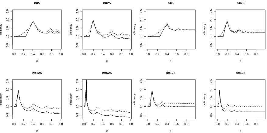
As the Dirichlet kernel (γj(κ)=1{j≤κ}) is of higher order forκ >1 — and so expected to be asymptotically more

effi_{cient — we have measured the e}ffi_{ciency of other kernels relative to this one. In Figure 1 we show the relative}

effi_{ciency of the von Miseswrapped normal (}γj(κ) = κj

2

), and Fej´er (γj(κ) = 1{j≤κ}(κ+1− j)/(κ+1)) kernels for

n = ₅,25,125,625 for the von Mises and wrapped Cauchy (αj = ρj;δj = 0) distributions. Not surprisingly, the

wrapped Normal and von Mises kernels are very similar, and both are better than the Fej´er kernel. For small n, the

von Mises kernel is more effi_{cient that the Dirichlet kernel; markedly so for the Cauchy distribution, or for data with}

low concentration.

3. Local polynomial regression

3.1. Linear fitting with von Mises based kernels

Consider the dataset{(Θ_i,Yi),i = 1,· · ·,n}, whereΘi := (Θi1,· · ·,Θid)T, and Yi ∈ Rare both observable,

ab-solutely continuous, random variables taking values respectively in [0,2π)d_and

R. ¿From now on we will assume

that

Yi=m(Θi)+σ(Θi)εi, i=1,· · ·,n

0.0 0.2 0.4 0.6 0.8 1.0 0.5 1.0 1.5 2.0 2.5 n=5 ρ efficiency

0.0 0.2 0.4 0.6 0.8 1.0

0.5 1.0 1.5 2.0 2.5 n=25 ρ efficiency

0.0 0.2 0.4 0.6 0.8 1.0

0.5 1.0 1.5 2.0 2.5 n=125 ρ efficiency

0.0 0.2 0.4 0.6 0.8 1.0

0.5 1.0 1.5 2.0 2.5 n=625 ρ efficiency

0.0 0.2 0.4 0.6 0.8

0.5 1.0 1.5 2.0 2.5 n=5 ρ efficiency

0.0 0.2 0.4 0.6 0.8

0.5 1.0 1.5 2.0 2.5 n=25 ρ efficiency

0.0 0.2 0.4 0.6 0.8

0.5 1.0 1.5 2.0 2.5 n=125 ρ efficiency

0.0 0.2 0.4 0.6 0.8

0.5 1.0 1.5 2.0 2.5 n=625 ρ efficiency

Figure 1: Relative effi_{ciency of Fej´er (——), wrapped normal (- - - - -), and von Mises (}· · ·) kernels to the Dirchlet kernel, for various values of n. With respect to the underlying true density, the left group corresponds to the von Mises distribution withρ=I1(ν)/I0(ν), while the right group

corresponds to the wrapped Cauchy distribution.

whereσ2_{(·) is the conditional variance of Y andε}

is are real-valued random variables with zero mean and unit variance.

Our objective is to construct an estimator of m(θ) as a function of the dataset when bothΘ_{is and}εis are i.i.d..

LetPθ(·;β) :=β0+Pdj=1βjsin(· −θj), and suppose that m(ψ) ≃ Pθ(ψ;β) forψin a neighborhood ofθ. Here

Pθ(θ;β)=β0, which motivates estimating m(θ) by ˆβ0. Recalling that for very small values ofθwe have sin(θ)≃θ,

then a Taylor series expansion justifies both ˆβ0and the values ˆβj, j=1,· · ·,d, as estimates of the partial derivatives

βj =∂m(θ)/∂θj. Viewed as local least squares estimators, ˆβ0,· · ·,βˆd minimizePin=1{Yi− Pθ(Θi;β)}2w(Θi,θ) where

w(Θ_i,θ) is the weight function, (a symmetric, continuous function integrating to 1) which, if strictly positive, decreases

with some distance betweenΘ_iandθ. Now we provide an explicit expression for ˆβ0together with its L2properties.

Let y :=_{(Y1,· · ·,Yn)}T_{be the response vector,}

Θ:=

   

1 sin(Θ₁₁−θ1) · · · sin(Θ1d−θd)

..

. ... ... ...

1 sin(Θ_{n1−θ1) · · · sin(}Θ_nd−θd)

   

the design matrix, and

W :=_diag{KC(Θ₁−θ),· · ·,KC(Θ_n−θ)}

the weight matrix, where C :=_{κI, I denoting the identity matrix of order d, and}

KC(Θ_i−θ) :=

d

Y

j=1

Kκ(Θi j−θj), i=1,· · ·,n. (3)

The local linear kernel estimator of m(θ) is given by the first entry of the vector

ˆ

β:=_{arg min}

β

n

X

i=1

(Yi−βTΘ)2KC(Θi−θ),

whereβ:=_{(β0, β1,· · · , βd)}T_{.Assuming the non-singularity ofΘ}T_{WΘ, standard weighted least squares theory yields}

ˆ

β=₍ΘT_WΘ)−1_ΘT_{W y,and}

ˆ

m(θ; C)=_eT

j(Θ

T_WΘ)−1_ΘT_{W y, (4)}

where ejis a (d+1)×1 vector having 1 as the jth entry and 0 elsewhere.

Given its effi_{ciency, as well as its prevalence in kernel smoothing of circular data, we firstly give results when the}

von Mises kernel Vκ(·) :=exp{κcos(·)}/{2πI0(κ)}is used to define the d-dimensional weight function.

Theorem 2. Given the dataset{(Θ_i,Yi),i = 1,· · ·,n}, where Θis are i.i.d. observations from the circular design

density f , and Yis are i.i.d. real-valued random variables , take the local linear kernel regression estimator ˆm(·; C)

equipped with the weight function VC(Θ_i−θ) :=Qd

j=1Vκ(Θi j−θj). Assume that

i) limn→∞κ−1=0;

ii) limn→∞n−1κd/2=0;

iii) the conditional varianceσ2_{is continuous, and the density f is continuously differentiable;}

iv) all second-order derivatives of the regression function m are continuous.

Then atθ∈[0,2π)d_{the conditional mean squared error of ˆm(θ; C) is given by}

E[{m(·ˆ ; C)−m(θ)}2|Θ₁,· · ·,Θ_n]=1

4

(_I

1(κ)

κI0(κ)

)2

tr2{Hm(θ)} +

" _I

0(2κ)

2π{I0(κ)}2

#d

σ2_(θ)

n f (θ) +op

κ−2+_n−1_κd/2_{, (5)}

where Hm(θ) denotes the Hessian matrix of m atθ.

Proof. See Appendix.

Once more, in the proof of the above theorem a major technical issue is that the concentration parameterκcannot

be “separated” from the kernel.

Remark 5. Sinceκ corresponds to the inverse of the squared bandwidth of the euclidean smoother, the remainder

term in (5) is consistent with that obtained by Ruppert&Wand (1994).

Finally, the optimal smoothing degree is given by

Corollary 1. The concentration parameter which minimizes the asymptotic mean squared error, i.e. the first two

summands in RHS of formula (5), is

"

tr4{Hm(θ)}{n f (θ)}222dπd

d2_σ4_(θ)

#1/(4+d)

.

Proof. See Appendix.

3.2. Generalizations and extensions

The results of Theorem 2 can be generalized to the class of second-order circular kernels Kκ. Given the

square-integrable function g, define R(g) :=R _g2_{, then}

Theorem 3. Given the dataset{(Θ_i,Yi),i = 1,· · ·,n}, where Θis are i.i.d. observations from the circular design

density f , and Yis are i.i.d. real-valued random variables, take the local linear kernel regression estimator ˆm(·; C)

equipped with the weight function in (3) with Kκ being a second-order circular kernel. Assume conditions i) of

Theorem 1, and iii) of Theorem 2, together with

i) limn→∞n−1R(KC)=0.

Then, atθ∈[0,2π)d,

E[{m(·ˆ ; C)−m(θ)}2|Θ₁,· · ·,Θ_n]= 1

16{1−γ2(κ)}

2_tr2_{H m(θ)}+

R(KC)σ2(θ)

n f (θ) +op(1).

Proof. See Appendix.

It would be of interest to determine the optimal smoothing degree in this case, but since the coeffi_cientsγjs

depend onκin a specific way for each kernel, the result in Corollary 1 is hard to generalize. Concerning the extension

Theorem 4. Given the dataset {(Θ_i,Yi),i = _{1,· · ·,n}, where} Θ_{is are i.i.d. observations from the circular}

one-dimensional density f , and Yis are i.i.d. real-valued random variables, take the local pth degree polynomial regression

estimator ˆm(·;κ) equipped with a second-order circular kernel Kκ. Assume conditions i) of Theorem 1, iii) and iv) of

Theorem 2. Moreover, assume that

i) for the kernelK(p)in Remark 2,limn→∞n−1R(K(p))=0;

ii) m(p+2)_{is continuous in a neighborhood ofθ.}

Then, for anyθ∈[0,2π),

E[ ˆm(θ;κ)−m(θ)|Θ_1,· · ·,Θ_n]=

  

ηp+1(K(p))m

(p+1)_(θ)

(p+1)! +op(1), if p is odd;

ηp+2(K(p))

m(p+1)_{(θ) f}′_(θ)

f (θ)(p+1)! + m(p+2)_(θ)

(p+2)!

+_{op(1), otherwise;}

and

Var[ ˆm(θ:κ)|Θ₁,· · ·,Θ_n]=R(K(p))

σ2_(θ)

n f (θ){1+op(1)}.

Proof. See Appendix.

4. Simulation results

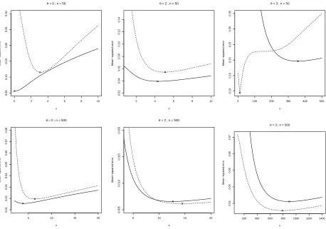
We briefly explore the asymptotic result given by Theorem 2 in a simulation study. We first investigate the

dependence of the mean squared error onθ,n andκwhen d=_{1 and choose a sharp-peaked response}

m(θ)=₂+_{sin (θ−1.2π)}+_{3 exp}

 

−10 15(θ−π)

2π

!2



,

withεi∼N(0,1),σ2(Θi)=1/2, andΘi, i=1,· · ·,n coming from a von Mises density with meanπand concentration

parameter 1. We estimate m(θ) at θ = _{0,2,3 and compare the average squared error of (4) with the asymptotic}

mean squared error given in Theorem 2 overκ for n = _{50 and n} = _{500. The results are displayed in Figure 2,}

and the asymptotic nature of the result is clear. Note that the values of the second derivative of m atθ= _{0,2,3 are}

−0.59,0.98,140.89, respectively, which explains the poorer performance atθ=_3.

Secondly, we explore the dependence on d. In this case we use the model

m(θ)=1

d

d

X

i=1

sinθi+

1

d(d−1) X

i,j

cosθicosθj (d≥2)

whereθ =₍θ1,· · ·, θd)T,σ2(Θi) =1/2, i =1,· · ·,n, and f is a product of (independent) von Mises densities with

mean zero and concentration parameter 1. We estimate m(θ) atθ=₍₀,· · ·,0)Tand (π/2,· · ·, π/2)Tfor a range ofκ,

for n=_{500. Figure 3 shows good agreement for d} =_{2 between the average squared error and the asymptotic mean}

squared error. However, we note increasingly poor behaviour as d increases, indicating that the asymptotic nature of the result also depends on d, and again illustrating the well-known phenomenon of the curse of dimensionality.

Appendix

Proof of Theorem 1. Express Kκ(θ) in terms of a Fourier series, and, recalling that for very small values of u

sin(u)≃u, use the expansion f (u+_θ)= _{f (θ)}+_{sin(u) f}′_(θ)+_{1/2 sin}2_{(u) f}′′_(θ)+_O{sin3_{(u)}. Then, starting from (2),}

make a change of variable and use assumption i) to get

E[ ˆf (θ;κ)]=

Z 2π

0

Kκ(ψ−θ) f (ψ)dψ

=

Z 2π

0

Kκ(u) f (u+θ)du

=_{f (θ)}+1

4{1−γ2(κ)}f

′′

(θ)+_o(1).

0 2 4 6 8 10

0.05

0.10

0.15

0.20

0.25

0.30

θ = 0 ; n = 50

κ

Mean−squared error

2 4 6 8 10

0.02

0.04

0.06

0.08

0.10

0.12

0.14

θ = 2 ; n = 50

κ

Mean−squared error

0 100 200 300 400 500

0.10

0.15

0.20

0.25

0.30

0.35

θ = 3 ; n = 50

κ

Mean−squared error

5 10 15 20

0.01

0.02

0.03

0.04

0.05

0.06

0.07

0.08

θ = 0 ; n = 500

κ

Mean−squared error

5 10 15 20

0.005

0.010

0.015

0.020

θ = 2 ; n = 500

κ

Mean−squared error

200 400 600 800 1000 1200 1400

0.03

0.04

0.05

0.06

0.07

θ = 3 ; n = 500

κ

Mean−squared error

Figure 2: Comparison of averaged squared error as a function ofκover 200 simulations (dashed line), and asymptotic mean squared error given by Theorem 2 (continuous line) with locations of minima. Top row: n=_{50; lower row: n}=_{500, with m estimated atθ}=_{0 (left),θ}=_{2 (middle) and} θ=_{3 (right).}

0 5 10 15 20

0.00

0.02

0.04

0.06

0.08

0.10

θ = 0 ; n = 500

κ

Mean−squared error

4

4

3 3

2 2

0 5 10 15 20

0.0

0.1

0.2

0.3

0.4

0.5

0.6

θ = π2 ; n = 500

κ

Mean−squared error

4

4 3

3 2

2

Figure 3: Comparison of averaged squared error as a function ofκover 200 simulations (dashed line), and asymptotic mean squared error given by Theorem 2 (continuous line) with locations of minima shown by the integers 2, 3, 4 which corresponds to the dimension of the data. m is estimated atθ=_(0,· · ·,0)T_{(left) andθ}=_(π/2,· · ·, π/2)T_(right).

Now, recalling assumptions i) and ii), we have

Var[ ˆf (θ;κ)]= 1

n

Z 2π

0

{Kκ(ψ−θ)}2f (ψ)dψ−

1

n

n

E[ ˆf (θ;κ)]o2

=1

n

Z 2π

0

{Kκ(u)}2{f (θ)+o(1)}du−

1

n{f (θ)

+_o(1)}2

= 1

2nπ

 

1+₂

∞

X

j=1

γ2_j(κ)  

f (θ)+_o(1).

Proof of Theorem 2. Put

SΘ_i−θ:={sin(Θi1−θ1),· · ·,sin(Θid−θd)}T, i=1,· · ·,n

and use Dg(θ) to denote the first-order partial derivatives vector of the function g atθ. To derive the conditional bias,

we firstly note that (4) yields

E[ ˆm(θ; C)|Θ₁,· · ·,Θ_n]=_eT

1(Θ

T

WΘ)−1ΘTW m, (6)

where m :=_{m(Θ₁),· · ·,m(Θ_n)}T_{,and W :=diag{V}

C(Θ1−θ),· · ·,VC(Θn−θ)}. Using the expansion

m=Θ "

m(θ)

Dm(θ)

# +1 2     ST

Θ₁−θHm(θ)SΘ1−θ .. .

ST

Θ_n−θHm(θ)SΘn−θ   

+Rm(θ),

where Rm(θ) denotes the remainder, we have that the first term in the expansion of (6) is m(θ). Thus

E[ ˆm(θ; C)−m(θ)|Θ₁,· · ·,Θ_n]= 1

2e

T

1(Θ

T

WΘ₎−1ΘT_W          ST

Θ₁−θHm(θ)SΘ1−θ .. .

ST

Θ_n−θHm(θ)SΘn−θ   

+Rm(θ)

     . Observe that

ΘTWΘ=

" Pn

i=1VC(Θi−θ) Pni=1VC(Θi−θ)STΘ_i−θ

Pn

i=1VC(Θi−θ)SΘ_i−θ Pni=1VC(Θi−θ)SΘ_i−θSTΘ_i−θ

#

(7)

and

ΘT_W    

ST

Θ₁−θHm(θ)SΘ1−θ .. .

ST

Θ_n−θHm(θ)SΘn−θ    =    Pn

i=1VC(Θi−θ)STΘ_i−θHm(θ)SΘi−θ

Pn

i=1VC(Θi−θ)

n

ST

Θ_i−θHm(θ)SΘi−θ o

SΘ_i−θ

 

, (8)

then, using the expansion

f (u+_θ)= _{f (θ)}+_ST

uDf(θ)+O(STuSu),

and recalling assumption i), a change of variables leads to these approximations

1

n

n

X

i=1

VC(Θi−θ)=

Z

[0,2π)d

VC(α−θ) f (α)dα+op(1)

=_{f (θ)}+_op(1);

1

n

n

X

i=1

VC(Θ_i−θ)SΘ_i−θ=

Z

[0,2π)d

VC(α−θ)Sα−θf (α)dα+op(1)

=I1(κ)

I0(κ)

C−1Df(θ)+op(C−11) ;

1

n

n

X

i=1

VC(Θ_i−θ)SΘ_i−θSTΘ_i−θ=

Z

[0,2π)d

VC(α−θ)Sα−θSTα−θf (α)dα+op(I)

= I1(κ)

I0(κ)

C−1f (θ)+_op(C−1_);

1

n

n

X

i=1

VC(Θ_i−θ)STΘ_i−θHm(θ)SΘ_i−θ=

Z

[0,2π)d

VC(α−θ)ST_α−θHm(θ)Sα−θf (α)dα+op(1)

= I1(κ) κI0(κ)

tr{Hm(θ)}f (θ)+op

κ−1;

1

n

n

X

i=1

VC(Θ_i−θ)nSTΘ_i−θHm(θ)SΘ_i−θ

o

SΘ_i−θ=

Z

[0,2π)d

VC(α−θ)nST_α−θHm(θ)Sα−θ

o

Sα−θf (α)dα+op(1)

=_Op(C−2_{1) ;}

where 1 is the unit vector of length d. Hence, recalling assumption i) we have

eT₁n−1ΘTWΘ−1_⋍h {f (θ)}−1_+o

p(1) −Df(θ)T{f (θ)}−2+op(1)

i

, (9)

thus

E[ ˆm(θ; C)−m(θ)|Θ₁,· · ·,Θ_n]=1

2

I1(κ)

κI0(κ)

tr{Hm(θ)}+op(κ−1).

For the conditional variance, according to multivariate local linear regression theory

Var[ ˆm(θ; C)|Θ₁,· · ·,Θ_n]=_eT

1(Θ

T

WΘ₎−1ΘT_WΣ_WΘ₍ΘT_WΘ₎−1_e1,

whereΣ:=_diag{σ2_(Θ

1),· · ·, σ2(Θn)}. Consider that

n−1ΘTWΣWΘ=

" _n−1Pn

i=1{VC(Θi−θ)}2σ2(Θi) n−1Pni=1{VC(Θi−θ)}2STΘ_i−θσ

2_(Θ i)

n−1Pn_i=1{VC(Θi−θ)}2SΘ_i−θσ2(Θi) n−1Pni=1{VC(Θi−θ)}2SΘ_i−θSTΘ_i−θσ

2_(Θ i)

#

, (10)

and approximate the components of the above matrix using the following relationships

1

n

n

X

i=1

{VC(Θ_i−θ)}2σ2(Θ_i)=

Z

[0,2π)d

{VC(Θ_i−θ)}2σ2(α) f (α)dα+_op(1)

=

" _I

0(2κ)

2π{I0(κ)}2

#d

σ2(θ) f (θ){1+_op(1)};

1

n

n

X

i=1

{VC(Θi−θ)}2STΘ_i−θσ

2_(Θ i)=

Z

[0,2π)d

{VC(αi−θ)}2STα−θσ

2₍

α) f (α)dα+_op(1)

=_{op(1) ;}

1

n

n

X

i=1

{VC(Θ_i−θ)}2SΘ_i−θSTΘ_i−θσ

2

(Θ_i)=

Z

[0,2π)d

{VC(αi−θ)}2Sα−θSTα−θσ

2

(α) f (α)dα+_op(I)

= Fe(2, κ

2₎

4π{I0(κ)}2

"

I0(2κ)

2π{I0(κ)}2

#d−1

σ2(θ) f (θ){I+_op(I)},

whereFe(2, κ2_{) := {I}

0(k)}2+{I1(k)}2+2P∞j=2Ij(κ){Ij(κ)− Ij−2(κ)}is the regularized confluent hypergeometric

function of the first kind. Combining the previous results with the approximations in (9), and recalling assumption ii), we finally obtain

Var[ ˆm(θ; C)|Θ₁,· · ·,Θ_n]=

"

I0(2κ)

2π{I0(κ)}2

#d

σ2_(θ)

n f (θ)+op(n

−1_κd/2_).

Proof of Corollary 1. ReplaceI1(κ)/I0(κ) by 1 with an error of magnitude O(κ−1), and use

lim

κ→∞

" _I

0(2κ)

2π{I0(κ)}2

#d

=

_κ

4π

d/2

,

then minimize the asymptotic MSE.

Proof of Theorem 3. Follow the proof of Theorem 2, with KC(Θi−θ) as ith entry of the weight matrix, i=1,· · ·,n.

In particular, to derive the conditional bias firstly note that

n−1ΘTWΘ_⋍ "

f (θ)+_{op(1) 1/2{1−γ2(κ)}D}T

f(θ)+op(1)

1/2{1−γ2(κ)}Df(θ)+op(1) 1/2{1−γ2(κ)}f (θ)I+op(I)

#

,

and, in virtue of assumption i) of Theorem 1,

eT₁(n−1ΘTWΘ)−1⋍h {f (θ)}−1+_{op(1) −D}T

f(θ){f (θ)} −2_+o

p(1)

i

.

Moreover, observe that

n−1ΘT_W    

ST

Θ₁−θHm(θ)SΘ₁−θ

.. .

ST

Θ_n−θHm(θ)SΘn−θ   

≃

"

1/2{1−γ2(κ)}tr{Hm(θ)}f (θ)+op(1)

Op(1)

#

,

to get

E[ ˆm(θ; C)−m(θ)|Θ₁,· · ·,Θ_n]=1

4{1−γ2(κ)}tr{Hm(θ)}+op(1).

To derive the conditional variance, observe that the upper-left entry of the matrix (10) generalizes as

1

n

n

X

i=1

{KC(Θ_i−θ)}2σ2(Θ_i)⋍R(KC)σ2(θ) f (θ){1+_op(1)},

where R(KC)={R(Kκ)}d={(2π)−1(1+2P∞j=1γ

2 j(κ))}

d_{, the diagonal blocks are o}

p(1), whereas letting

A(KC) :=[γ

2 0(κ)+γ

2 1(κ)+2

P∞

j=2γj(κ){γj(κ)−γj−2(κ)}]{R(Kκ)}d−1

4π ,

whereγ0(κ) :=

R2π

0 Kκ(θ) cos(0)dθ=1, the lower-right entry is

1

n

n

X

i=1

{KC(Θ_i−θ)}2SΘ_i−θSTΘ_i−θσ

2_(Θ

i)⋍A(KC)σ2(θ) f (θ){I+op(I)}.

Hence, it finally results

Var[ ˆm(θ; C)|Θ₁,· · ·,Θ_n]=R(KC)σ

2_(θ)

n f (θ) {1+op(1)}.

Proof of Theorem 4. Follow the proof of Theorem 4.1 of Ruppert & Wand (1994) with these two recommendations:

in the design matrix replace (Xi−x)j, with sinj(Θi−θ), and use the expansion f (u+θ)= f (θ)+sin(u) f′(θ)+O{sin2(u)}.

In particular, to derive the conditional bias, let Qp be the matrix of order p+1 having as (i,j) entryηi+j−1(Kκ), and

observe that, in virtue of assumption i) of Theorem 1, n−1_ΘT_{WΘ = f (θ)E}

p+ f′(θ)Qp +op(1),with Ep being the

matrix defined in Remark 2, to get

rT₁(n−1ΘTWΘ)−1=_{f (θ)}−1_{rT

1E −1 p −f

′_{(θ) f (θ)}−1_rT

1E −1

p QpE−1p }+op(1),

where r1 is a (p+1)×1 vector having 1 as first entry and 0 elsewhere. For the conditional variance, denoting as

Tpthe matrix of order p+1 having

R

sini+j−2(u){Kκ(u)}2du as (i,j) entry, and recalling condition i), it follows that

n−1ΘT_W2_{Θ=f (θ)T}

p+op(I).

Aknowledgements

The authors are grateful to two anonymous referees for their valuable comments which led to improvements in this article.

References

Bai, Z. D., Rao, R. C. & Zhao, L. C. (1988), ‘Kernel estimators of density function of directional data’, Journal of Multivariate Analysis 27, 24–39. Beran, R. (1979), ‘Exponential models for directional data’, The Annals of Statistics 7, 1162–1178.

Cogburn, I. & Davis, H. T. (1974), ‘Periodic splines and spectral estimation’, The Annals of Statistics 2, 1108–1126. Hall, P., Watson, G. & Cabrera, J. (1987), ‘Kernel density estimation with spherical data’, Biometrika 74, 751–762. Jammalamadaka, S. R. & SenGupta, A. (2001), Topics in Circular Statistics, World Scientific, Singapore.

Klemel¨a, J. (2000), ‘Estimation of densities and derivatives of densities with directional data’, Journal of Multivariate Analysis 73, 18–40. Lejeune, M. & Sarda, P. (1992), ‘Smooth estimators of distribution and density functions’, Computational Statistics&Data Analysis 14, 457–471.

Mardia, K. V. & Jupp, P. E. (1999), Directional Statistics, John Wiley, New York.

Ruppert, D. & Wand, M. P. (1994), ‘Multivariate locally weighted least squares regression’, The Annals of Statistics 22, 1346–1370. Silverman, B. W. (1986), Density Estimation for Statistics and Data Analysis, Chapman and Hall, London.