Mid-infrared luminous quasars in the GOODS–
Herschel
fields: a large
population of heavily obscured, Compton-thick quasars at
z
≈
2
A. Del Moro,
1,2‹D. M. Alexander,
1F. E. Bauer,
3,4,5,6E. Daddi,
7D. D. Kocevski,
8D. H. McIntosh,
9F. Stanley,
1W. N. Brandt,
10,11,12D. Elbaz,
7C. M. Harrison,
1B. Luo,
13J. R. Mullaney
14and Y. Q. Xue
151Centre for Extragalactic Astronomy, Department of Physics, Durham University, South Road, Durham DH1 3LE, UK 2Max-Planck-Institut f¨ur Extraterrestrische Physik (MPE), Postfach 1312, D-85741 Garching, Germany
3Instituto de Astrof´ısica, Facultad de F´ısica, Pontificia Universidad Cat´olica de Chile, 306, Santiago 22, Chile 4Millenium Institute of Astrophysics, Vicu˜na Mackenna 4860, 7820436 Macul, Santiago, Chile
5EMBIGGEN Anillo, Concepci´on, Chile
6Space Science Institute, 4750 Walnut Street, Suite 205, Boulder, CO 80301, USA 7CEA-Saclay, F-91191 Gif-sur-Yvette Cedex, France
8Department of Physics and Astronomy, University of Kentucky, Lexington, KY 40506-0055, USA
9Department of Physics & Astronomy, University of Missouri-Kansas City, 5110 Rockhill Rd, Kansas City, MO 64110, USA 10Department of Astronomy and Astrophysics, 525 Davey Lab, Pennsylvania State University, University Park, PA 16802, USA 11Institute for Gravitation and the Cosmos, Pennsylvania State University, University Park, PA 16802, USA
12Department of Physics, Pennsylvania State University, University Park, PA 16802, USA 13School of Astronomy and Space Science, Nanjing University, Nanjing 210093, China
14Department of Physics and Astronomy, University of Sheffield, Hounsfield Road, Sheffield S3 7RH, UK
15Key Laboratory for Research in Galaxies and Cosmology, Department of Astronomy, University of Science and Technology of China, Chinese Academy of
Sciences, Hefei, Anhui 230026, China
Accepted 2015 November 19. Received 2015 November 19; in original form 2015 April 2
A B S T R A C T
We present the infrared (IR) and X-ray properties of a sample of 33 mid-IR luminous quasars (νL6µm≥6×1044erg s−1) at redshiftz≈1–3, identified through detailed spectral energy distribution analyses of distant star-forming galaxies, using the deepest IR data fromSpitzer
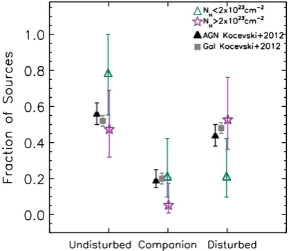
andHerschelin the GOODS–Herschelfields. The aim is to constrain the fraction of obscured, and Compton-thick (CT,NH>1.5×1024cm−2) quasars at the peak era of nuclear and star for-mation activities. Despite being very bright in the mid-IR band,≈30 per cent of these quasars are not detected in the extremely deep 2 and 4 MsChandraX-ray data available in these fields. X-ray spectral analysis of the detected sources reveals that the majority (≈67 per cent) are ob-scured by column densitiesNH>1022cm−2; this fraction reaches≈80 per cent when including the X-ray-undetected sources (9 out of 33), which are likely to be the most heavily obscured, CT quasars. We constrain the fraction of CT quasars in our sample to be≈24–48 per cent, and their space density to be=(6.7±2.2)×10−6Mpc−3. From the investigation of the quasar host galaxies in terms of star formation rates (SFRs) and morphological distortions, as a sign of galaxy mergers/interactions, we do not find any direct relation between SFRs and quasar luminosity or X-ray obscuration. On the other hand, there is tentative evidence that the most heavily obscured quasars have, on average, more disturbed morphologies than the un-obscured/moderately obscured quasar hosts, which preferentially live in undisturbed systems. However, the fraction of quasars with disturbed morphology amongst the whole sample is ≈40 per cent, suggesting that galaxy mergers are not the main fuelling mechanism of quasars atz≈2.
Key words: galaxies: active – quasars: general – galaxies: star formation – infrared: galaxies – X-rays: galaxies.
E-mail:[email protected]
1 I N T R O D U C T I O N
Since the discovery that most, if not all, galaxy spheroids in the local Universe host a supermassive black hole (SMBH) whose mass
C
scales with that of the host-galaxy bulge (e.g. Magorrian et al.1998; Ferrarese & Merritt2000; Marconi & Hunt2003) it has been clear that there is likely to be a tight connection between the evolution of SMBHs and galaxies. Studies of the galaxy population across cosmic time have shown that galaxies were more actively growing in the past, as the star formation rate (SFR) density peaks at redshift z≈2 and rapidly declines to the present day (e.g. Madau et al.1996; Hopkins et al.2006). A similar evolution is seen in the moderate-to-high luminosity active galactic nucleus (AGN) population, where most of the SMBHs accrete more rapidly at high redshift (z1–2), becoming more quiescent atz=0 (e.g. Brandt & Alexander2015, and references therein). Whether this parallel evolution between galaxies and SMBHs is simply due to a larger gas supply to feed both black hole accretion and star formation (SF) at high redshift, or whether there are other processes that self-regulate the SMBH and galaxy growth is still uncertain (e.g. Alexander & Hickox2012; Kormendy & Ho2013). A complete census of AGN is crucial to fully understand the accretion history of the SMBHs and their role in galaxy evolution. However, as the Universe at high redshift is more gas and dust rich, most of the accretion on to SMBHs is expected to be heavily obscured, which makes the identification and study of a large fraction of the AGN population very challenging.
X-ray observations provide arguably the most efficient way to trace the growth of SMBHs, as the high-energy radiation can pene-trate large amounts of gas and dust without significant absorption. Moreover, the contamination from galaxy emission at X-ray ener-gies is small as galaxies are typically much fainter than AGN in this band. However, when the column density of the obscuring mate-rial becomes Compton thick (CT;NH>1.5×1024cm−2) even the deepest X-ray surveys often fail to detect the population of the most obscured, CT AGN (e.g. Xue et al.2012; see Brandt & Alexander
2015for a review). A significant fraction of such AGN is predicted by all models of the cosmic X-ray background (CXB) to reproduce the observed background spectrum at high energies (E≈30 keV; e.g. Comastri et al.1995; Gilli, Comastri & Hasinger2007; Treis-ter, Urry & Virani2009), however, the actual contribution from CT AGN is not well constrained and varies between the models, due to different assumptions, and the space density of CT AGN is still uncertain.
Since most of the absorbed AGN emission is re-emitted in the mid-infrared band (MIR;λ≈3–40µm) by the circumnuclear dust heated by the central SMBH, observations in this band can poten-tially identify the elusive CT AGN missed by X-ray surveys (e.g. Lacy et al.2004; Stern et al.2005; Alexander et al.2008; Donley et al.2008,2012; Fiore et al.2008; Georgantopoulos et al.2011a; Mateos et al.2013). Moreover, since the infrared (IR) band is much less affected by extinction than the UV, optical and soft X-ray bands, the selection of AGN in the MIR band is almost unbiased against obscured AGN. The downside of using the IR band to study AGN is the strong contamination from SF in the host galaxies, whose cold dust emission tends to dominate the MIR to far-IR (FIR,λ≈ 40–250µm) bands, peaking atλ≈100–160µm. This is especially the case for low-to-moderate luminosity AGN, whose IR emission is often swamped by SF. These sources are easily missed by typical MIR colour–colour sample selection, which are generally used to identify AGN within the star-forming galaxy (SFG) population (e.g. Lacy et al.2004; Stern et al.2005; Donley et al.2012; Mateos et al.
2013).
In this paper, we investigate a sample of MIR luminous quasars (hereafter, ‘IR quasars’) at redshift z≈ 1–3, i.e. at the peak era of AGN and SF activity. We used the deepest available Spitzer
andHerscheldata in the GOODS–HerschelNorth and South fields
(hereafter, GH-N and GH-S, respectively; Elbaz et al. 2011) to reliably identify AGN in the MIR band through detailed spectral energy distribution (SED) analyses, which allow us to disentangle the AGN and SF emissions at MIR and FIR wavelengths. The SED analysis is a much more powerful tool than the simple IR colour– colour techniques for identifying AGN, as it can recover the hot dust emission from the AGN even when it does not strongly dominate the SED (e.g. Del Moro et al.2013; Rovilos et al.2014); however even the SED analyses have limitations and become incomplete when the AGN component is faint compared to the SF component. Using the deepestChandraX-ray data available across the sky (2 Ms in CDF-N; Alexander et al.2003; and 4 Ms in CDF-S; Xue et al.2011), we investigate the X-ray spectra of the IR quasars to constrain the fraction of obscured and CT sources. We also investigate the properties of their host galaxies to place them in the context of potential SMBH-galaxy evolution scenarios. The paper is organized as follows: in Section 2 the data used in our analyses are described, while Section 3 details the SED analysis method and the selection of our IR quasar sample. Section 4 presents the X-ray spectral analysis and results for our quasars, as well as the properties of their host galaxies assessed by the SFRs derived from our SED analyses, and their morphologies, obtained from visual classification ofHST -WFC3K-band images. In Section 5, the results obtained from our analyses are discussed in the wider context of the CXB models and the SMBH-galaxy evolutionary scenario. A summary and final remarks are given in Section 6. Throughout the paper we assume a cosmological model withH0 =70 km s−1Mpc−1, M = 0.27 and=0.73 (Spergel et al.2003). All the errors are quoted at a 90 per cent confidence level, unless otherwise stated.
2 DATA
2.1 IR observations
The GOODS fields have been observed in the IR band by theSpitzer
andHerschelspace observatories, and include the deepest IR data currently available. TheSpitzerobservations (Giavalisco et al.2004) cover the MIR band at 3.6, 4.5, 5.8 and 8.0µm with IRAC (Fazio et al.2004) and at 24µm with MIPS (Rieke et al.2004) as part of the GOODS Legacy programme (PI: M. Dickinson). The 24µm source catalogue was created using a point spread function (PSF) fitting technique at the 3.6µm source positions as priors (>5σdetections). For details of the observations and catalogue, we refer to Magnelli et al. (2009,2011). In both fields, the 24µm observations reach a point source sensitivity limit of∼30µJy (5σ).
FIR observations of the GOODS fields were undertaken by Her-schelas part of the GOODS–Herschelsurvey project (GH; Elbaz et al.2011). The GH survey covers the full≈10 arcmin×16 arcmin GOODS-N field with PACS (Poglitsch et al.2008) at 100 and 160
µm and with SPIRE (Griffin et al.2010) at 250, 350, 500µm, for a total observing time of 124 h. In GOODS-S a smaller region of
≈10 arcmin×10 arcmin at the centre of the field was observed by PACS at 100 and 160µm and the total exposure was 206.3 h (GH-S; Elbaz et al.2011). We also used the SPIRE 250µm data observed as part of theHerschelMulti-tiered Extragalactic Survey (Oliver et al.2012) across the GH-S field, to better match the data available in GH-N. We note that since the SPIRE data suffer from significant flux blending issues, we limit our analyses to the 250µm band in both the GH-N and GH-S fields, where these issues can still be corrected fairly well.
PSF fitting (courtesy of E. Daddi). In the GH-N field 819 sources (∼42 per cent of the 24µm priors) are detected in at least one of the
Herschelbands down to 5σ (3σ) sensitivity limits of∼1.7 (∼1.2) mJy,∼4.5 (∼2.3) mJy and∼6.5 (∼4.0) mJy, respectively. In the GH-S field there are 591 sources (∼34 per cent of the 24µm priors) detected byHerschel(at 100, 160 or 250µm); the faintest sources are detected down to 5σ (3σ) flux densities of 1.3 (0.7), 2.7 (1.7), 7.7 (5.0) mJy in the three bands, respectively; however, for general sources the flux densities and errors are higher, depending on the local source density and the de-blending uncertainties. In case of non-detection in any of theHerschelbands, appropriate flux density upper limits were calculated for each prior position.
In our analyses we initially considered all the 24µm-detected sources within the GH fields, namely 1943 sources in GH-N and 1747 sources in GH-S (for a total of 3690 sources), with or without aHerscheldetection. For the sample in GH-N≈98 per cent of the sources have a redshift identification, of which≈63 per cent are spectroscopic redshifts, while the remaining are photometric (see Del Moro et al.2013, hereafterDM13, for a detailed description of the redshift compilation). In the GH-S field, a redshift iden-tification is available for≈86 per cent of the sources, of which
≈95 per cent are spectroscopic redshifts compiled from multiple catalogues available in the literature (Le F`evre et al.2004; Mignoli et al.2005; Vanzella et al.2008; Popesso et al.2009; Balestra et al.
2010; Silverman et al.2010; Xia et al.2011) and 5 per cent are photometric redshifts.
2.2 X-ray observations
The X-ray counterparts for the 24µm-detected sources in GH-N and GH-S were found by cross-matching the 24µm positions with the X-ray source catalogues by Alexander et al. (2003) in the
ChandraDeep Field North (CDF-N), constructed from the 2 Ms
Chandraobservations covering an area of∼448 arcmin2of the sky, and by Xue et al. (2011) in theChandraDeep Field South (CDF-S), from the 4 MsChandradata over a region of 464.5 arcmin2. The CDF-N catalogue contains 503 X-ray-detected sources, down to flux limits off0.5−2 keV≈2.5×10⁻¹⁷erg cm−2s−1andf2−8 keV≈ 1.4×10⁻¹⁶ erg cm−2 s−1. The CDF-S X-ray source catalogue contains 740 sources down to flux limits of f0.5−2 keV≈9.1× 10⁻¹⁸erg cm−2s−1andf
2−8 keV≈5.5×10⁻¹⁷erg cm−2s−1. For details on the data reduction and the construction of the catalogues we refer to Alexander et al. (2003), Luo et al. (2008) and Xue et al. (2011).
For the X-ray-detected sources in our sample (see Section 3.2), X-ray spectra have been extracted and analysed. The data were processed using theChandraInteractive Analysis of Observations1 (CIAO; version 4.3 and CALDB4.4.1; Fruscione et al. 2006) tools and the ACIS Extract (AE) software package2(Broos et al.2010, 2012). TheChandraspectra were produced using theAEsoftware (version 2011-03-16), extracting source and background spectra in each individual observation, as well as the relative response matrices and ancillary files, and combining them using theFTOOLS3addrmf andaddarf(Blackburn1995).
1http://cxc.cfa.harvard.edu/ciao/index.html
2The ACIS Extract software package and users guide are available at
http://www.astro.psu.edu/xray/acis/acis_analysis.html.
3http://heasarc.gsfc.nasa.gov/ftools/
2.3 Optical/near-infrared observations
The GOODS-N and GOODS-S fields have been observed by the
Hubble Space telescope(HST) ACS camera as part of the GOODS project (Giavalisco et al.2004), and WFC3 camera as part of the Cosmic Near-Infrared Deep Extragalactic Legacy Survey (CAN-DELS), a large programme consisting of broad-band photometric UV to the near-IR imaging of five separate deep extragalactic fields (see Grogin et al. 2011 and Koekemoer et al.2011, for details on the observations and data reduction). The CANDELSHST ob-servations in the GOODS-N field cover an area of≈10 arcmin× 16 arcmin (CANDELS-Wide) with a deeper smaller region in the centre (CANDELS-DEEP;≈6.8 arcmin×10 arcmin). The imag-ing of the GOODS-S field covers a similar region as in GOODS-N, but also includes a small ultradeep area in the centre of the field (HubbleUltra-Deep field; 2 arcmin×2.3 arcmin). In this paper we mainly use data in theF125WandF160Wbands, which approxi-mately correspond to near-IRJandHbands, but also consider data from the opticalF606WandF850LPbands (corresponding to theV
andzbands, respectively), to corroborate our visual classification of the galaxy morphology (Section 4.4).
3 S E D A N D S A M P L E S E L E C T I O N
3.1 IR SED decomposition
To constrain the IR emission from the AGN and the host galaxies, our SED-fitting approach uses an empirical AGN template and five different SFG templates from Mullaney et al. (2011), which have been extended down to 3µm and to the radio band (DM13). The AGN template atλ40µm is represented by a broken power law, where the indices have been fixed at the average values of 1=1.7 and 2=0.7 and the power-law break atλ=19µm.4An extinction law (Draine2003) is also applied to the AGN template, with the extinction parameterAVfree to vary in the range ofAV=0–30 mag (Mullaney et al.2011;DM13). TheSpitzer8, 16 and 24µm and theHerschel100, 160 and 250µm photometric points are used to constrain the source SEDs (see FigsA1andA2in appendix); the
SpitzerIRAC flux densities at 3.6, 4.5 and 5.8µm are not included in the SED analysis because these data are likely to be dominated by starlight emission, which is not taken into account in our templates. The SEDs for all of the 24µm-detected sources with redshift measurements in the GH-N and GH-S fields have been initially fitted with the SFG templates only, and subsequently with the AGN+ SFG templates obtaining a best-fitting solution for each of the SFG templates, using aχ2-fitting technique (seeDM13, for details). We adopted the Bayesian information criterion (BIC; Schwarz1978) to assess the improvement of the fits due to the addition of the AGN component to each of the SFG templates, and therefore to identify the best-fitting model for each source. Namely, the AGN+SFG model is assumed as the best-fitting model if for each source:
4We also performed the SED fitting using
1as a free parameter for the
sources with enough data points in the MIR band to constrain the power-law slope. We note that this is not the case for all the sources, as atz
1.7 the 8µm data point falls out of the wavelength range covered by our SED templates. Moreover, in some cases the 16µm data are upper limits and therefore cannot provide strong constraints to the MIR power-law slope. However, where the fits with 1as free parameter provided a better
representation of the data compared to a fixed 1=1.7, we adopted these
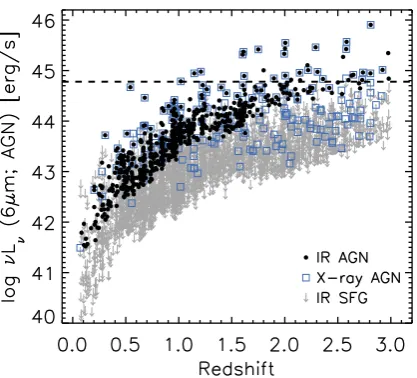
Figure 1. Rest-frame 6µm AGN luminosity, calculated from the SED fits, versus redshift for all of the 24µm-detected sources in the GH fields (∼3200 sources withz≤3, out of the total 3690 24µm-detected sources). The black circles represent the sources where we significantly identify an AGN component in the IR SED (Section 3.1), while the blue open squares represent the X-ray-detected AGN. For sources where an AGN component was not found in the best-fitting SEDs (‘IR SFG’), the 6µm AGN luminosity is plotted as an upper limit (grey arrows). The dashed line at logνL6µm=
44.78 erg s−1marks our threshold for the IR quasar selection.
(1)BICi=BICSFG,i−BICAGN+SFG,i>2 (e.g. Kass & Raftery 1995), wherei=1–5 refers to each of the SFG templates, in at least 4 out of the 5 pairs of best-fitting solutions;
(2) min(χ2
AGN+SFG,j)<min(χSFG2 ,i), withj≤i, i.e. the minimum χ2of the AGN+SFG solutions that satisfy condition (1) should be less than the minimumχ2obtained by fitting any of the SFG templates alone.
If any of these criteria is not met we conservatively adopt the sim-ple SFG model as the best-fitting model. These criteria are adopted to assess the reliability of the AGN component independently from the individual SFG templates. In fact, due to the sparse data points available for our SED analysis, in some cases, individual fitting solutions from different templates yield similarly good fit to the data, preventing us from identifying a unique best-fitting solution. We refer to section 3.1 and appendix A ofDM13, for a detailed description of the SED-fitting approach and tests on its reliability.5 After identifying the best-fitting model, we derived the luminosity of the AGN (i.e. corrected for the galaxy contribution) at rest-frame 6µm (L6µm,AGN), the IR luminosity of the AGN (LAGN) calculated across the wavelength rangeλ=8–1000µm, and the IR luminosity of the SFG (λ= 8–1000µm; hereafterLSF), as weighted means of the values obtained from the five best-fitting model solutions [or from all the solutions satisfying condition (1) for the AGN
+SFG model]. Where the AGN component was not significantly identified an upper limit to the AGN luminosity at 6µm was set as 50 per cent of the total 6µm emission (Fig.1), i.e. the limit for the SFG component becoming dominant at 6 µm. For the cases where the FIR data (100, 160 and 250µm) are all upper limits and
5We note that here we have slightly modified the criteria to evaluate the
reliability of the AGN component compared to those presented inDM13, by adopting the BIC instead of anf-test. The BIC is a more appropriate statistical criterion to compare the results from different models than the
f-test when the models are non-nested.
our SED-fitting approach did not provide a reliable measurement of the SF emission, we estimated an upper limit forLSFby increasing the normalization of the SFG templates until they reached any of the FIR upper limits, without exceeding any of the MIR data point measurements (including errors). An IR luminosity was calculated from each of the five templates and the highest value was then taken as theLSFupper limit.
3.2 IR quasar sample
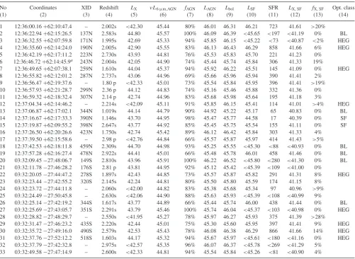
From the results obtained from our SED decomposition, we selected a sample of luminous AGN withνL6µm,AGN≥6×1044erg s−1(≥ 44.78 in the logarithmic scale; Fig.1), defined hereafter as our ‘IR quasar’ sample. Considering the intrinsic relation between the 6µm luminosity and the X-ray luminosity observed for unobscured AGN (e.g. Lutz et al.2004; Fiore et al.2009; Gandhi et al.2009; Mateos et al.2015), our 6µm luminosity cut corresponds to an intrinsic X-ray luminosityL2−10 keV≈2.5×1044erg s−1, i.e. clearly in the quasar regime even allowing for the≈0.4 dex scatter in the relation. We also restricted our sample to the redshift rangez=1–3 as we aim to investigate the population of luminous quasars at the peak of activity atz≈2 (Madau et al.1996; Hopkins et al.2006; Ueda et al.2014; Brandt & Alexander2015). Our sample consists of 33 sources, 19 in the GH-N and 14 in the GH-S fields (see Table1). The bolometric luminosities (Lbol) of these quasars, estimated as Lbol ≈ 2×LAGN(assuming a bolometric correction of a factor of ∼8 at 6 µm, from Richards et al. 2006, and considering the median ratio of∼0.3 betweenνL6µm,AGNandLAGNestimated for our quasars), span the range logLbol = 45.4–46.5 erg s−1 (see Table1). For all of these sources, we find that the AGN component largely dominates over the SF component at MIR wavelengths, with the AGN contributing>66 per cent to the total emission at 6µm (fAGN=66–100 per cent; wherefAGNis defined as the fraction of AGN luminosity over the total at rest-frame 6µm; see Table1). The best-fitting SEDs are reported in Appendix A (FigsA1andA2). We note that for 13 out of the 33 sources (≈40 per cent)Spitzer-IRS low-resolution spectroscopy is available (λ≈3–20µm; Pope et al.
2008a; Murphy et al.2009; Kirkpatrick et al.2012). Although we do not use these spectra to constrain the source SEDs, we find very good agreement between our SED best-fitting solutions and the
Spitzer-IRS spectra, which are shown in FigsA1andA2(Appendix A), confirming the reliability of our SED-fitting approach.
To explore the completeness of the sample we can take into ac-count that when the AGN is not dominant in the MIR band, i.e. its contribution to the total emission is<50 per cent, our SED-fitting procedure might start failing in identifying the presence of an AGN. We therefore looked for all the sources identified as SFGs from our SED-fitting procedure (i.e. with no significant AGN com-ponent) with AGN luminosity upper limits above our IR quasar selection threshold of log νL6µm,AGN≥44.78 erg s−1. There is only one SFG satisfying this condition, having log νL6µm,AGN< 44.85 erg s−1. This source is classified as an AGN from its X-ray emission (logLX ≈43.2 erg s−1). Given its modest X-ray lumi-nosity and since theL6µm,AGNupper limit is very close to our IR quasar luminosity threshold (only a factor of∼1.2 higher), the AGN within this SFG might still not fulfil our selection criteria, i.e. its intrinsic power could be below our luminosity cut. For this reason we do not include this source in our sample, keeping in mind that our selection might not be 100 per cent complete in identifying IR quasars when the SF luminosity is very high.
Table 1. IR quasar sample. (1) Source number; (2) MIR 3.6µm source position, RA and Declination; (3) X-ray source identification number from Alexander et al. (2003) in CDF-N and from Xue et al. (2011) in CDF-S; the suffix ‘N’ and ‘S’ refer to North and South, respectively; (4) redshift; ‘s’ and ‘p’ indicate the spectroscopic and photometric redshifts, respectively (Section 2.1); (5) logarithm of the X-ray luminosity at rest-frame 2–10 keV, extrapolated from the measured 0.5–2 keV flux (or upper limit), in units of erg s−1; (6) logarithm of the rest-frame 6µm luminosity of the AGN measured from the best-fitting SEDs
in units of erg s−1; (7) contribution from the AGN emission to the total (AGN+SF) emission at 6µm; (8) logarithm of the AGN IR luminosity (8–1000µm) in
units of erg s−1; (9) logarithm of the AGN bolometric luminosity, derived fromL
AGN, in units of erg s−1; (10) logarithm of the IR luminosity (8–1000µm) of
the star formation component in units of erg s−1; (11) star formation rate in units of M
yr−1; (12) logarithm of the rest-frame 2–10 keV luminosity produced
by SF, estimated assuming the Lehmer et al. (2010) relation between SFR and hard X-ray luminosity; (13) estimated contribution from SF to the rest-frame 2–10 keV luminosity (uncorrected for absorption); (14) optical spectroscopic classification from Steidel et al. (2002), Barger et al. (2003) and Trouille et al. (2008) for the sources in GH-N and from Szokoly et al. (2004) and Silverman et al. (2010) in GH-S: broad-line AGN (BL), high-excitation emission line galaxies (HEG); star-forming galaxies (SF).
No Coordinates XID Redshift LX νL6µm,AGN fAGN LAGN Lbol LSF SFR LX, SF fX, SF Opt. class
(1) (2) (3) (4) (5) (6) (7) (8) (9) (10) (11) (12) (13) (14)
1 12:36:00.16+62:10:47.4 – 2.002s <42.30 45.44 80% 46.01 46.31 46.21 723 41.61 >20% 2 12:36:22.94+62:15:26.5 137N 2.583s 44.80 45.57 100% 46.09 46.39 <45.65 <197 <41.19 0% BL 3 12:36:32.55+62:07:59.8 171N 1.995s 42.69 45.33 94% 45.85 46.15 <45.22 <73 <40.87 <2% HEG 4 12:36:35.60+62:14:24.0 190N 2.005s 42.90 45.55 83% 46.13 46.43 46.29 858 41.66 6% HEG 5 12:36:42.19+62:17:11.2 223N 2.730s 43.93 44.81 76% 45.53 45.83 45.70 221 41.23 0%
6 12:36:46.72+62:14:45.9a 243N 2.004s 42.05 44.90 74% 45.44 45.74 45.84 306 41.33 19%
7 12:36:49.65+62:07:38.1 259N 1.610s 44.04 45.37 94% 45.92 46.22 45.51 145 41.09 0% HEG 8 12:36:55.82+62:12:01.2 287N 2.737s 43.06 44.96 69% 45.66 45.96 45.94 390 41.41 2%
9 12:36:56.47+62:19:37.6 – 1.80 p <42.33 45.01 73% 45.54 45.84 45.95 396 41.41 >19% 10 12:36:57.93+62:21:28.7 299N 2.36 p 44.12 44.83 74% 45.16 45.46 45.88 332 41.36 0% 11 12:36:59.32+62:18:32.4 307N 2.14 p 42.74 44.96 83% 45.68 45.98 45.64 195 41.18 3%
12 12:37:04.34+62:14:46.2 – 2.214s <42.09 45.11 91% 45.85 46.15 45.41 114 41.01 >4% HEG 13 12:37:06.87+62:17:02.1 344N 1.019s 44.14 44.79 90% 44.92 45.22 45.17 65 40.83 0% BL 14 12:37:16.67+62:17:33.3 390N 1.146s 43.70 44.95 98% 45.47 45.77 44.58 17 40.39 0% SF 15 12:37:19.87+62:09:55.2 398N 2.647s 43.77 44.92 85% 45.45 45.75 45.54 155 41.11 0% SF 16 12:37:26.50+62:20:26.6 423N 1.750s 42.74 45.42 89% 46.12 46.42 45.84 303 41.33 4%
17 12:37:39.50+62:15:58.6 – 2.98 p <42.76 44.84 66% 45.57 45.87 45.97 414 41.43 >5% 18 12:37:42.53+62:18:11.8 459N 2.309s 44.70 44.98 93% 45.25 45.55 <45.30 <88 <40.93 0% BL 19 12:37:57.28+62:16:27.4 478N 2.922s 44.41 45.01 66% 45.48 45.78 46.01 458 41.46 0% BL 20 03:32:09.45−27:48:06.7 149S 2.810s 43.96 45.91 100% 46.22 46.52 <45.80 <280 <41.30 0% BL 21 03:32:11.78−27:46:28.2 176S 2.81 p 43.81 44.95 92% 45.12 45.42 <45.39 <109 <41.00 0%
22 03:32:20.05−27:44:47.2 278S 1.897s 42.43 44.85 73% 45.57 45.87 45.82 291 41.31 8% HEG 23 03:32:23.44−27:42:55.2 320S 2.145s 42.24 44.81 80% 45.50 45.80 45.59 174 41.15 8%
24 03:32:23.72−27:44:11.8 – 2.060s <42.00 44.82 83% 45.38 45.68 45.34 97 40.96 >9% 25 03:32:24.49−27:50:45.8 – 2.630s <42.06 44.90 88% 45.63 45.93 <45.39 <108 <40.99 9%
26 03:32:25.14−27:42:19.2 344S 1.617s 43.77 44.89 66% 45.44 45.74 46.00 438 41.44 0% BL 27 03:32:25.69−27:43:05.7 351S 2.291s 43.79 45.46 100% 45.74 46.04 <45.37 <103 <40.98 0% HEG 28 03:32:28.82−27:48:29.7 – 2.550s <41.95 45.27 78% 45.97 46.27 45.93 375 41.39 >28%
29 03:32:31.47−27:46:23.2 435S 2.220s 42.44 45.01 75% 45.30 45.60 45.95 397 41.41 9% HEG 30 03:32:35.72−27:49:16.0 490S 2.579s 42.53 45.43 78% 46.08 46.38 46.29 866 41.66 14% HEG 31 03:32:37.76−27:52:12.2 518S 1.603s 44.17 45.32 94% 45.67 45.97 <45.61 <180 <41.16 0% HEG 32 03:32:37.79−27:42:32.8 – 2.975s <42.57 45.35 96% 46.07 46.37 <45.78 <269 <41.29 5%
33 03:32:49.58−27:47:14.9 – 2.600s <42.33 44.81 94% 45.54 45.84 <45.26 <81 <40.90 4%
Notes:aFor this source, we report the X-ray coordinates as the 3.6µm coordinates are centred on a low-redshift galaxy (z=0.556) lying≈1.8 arcsec from the X-ray source. Careful inspection of the multiwavelength images has proved that although theSpitzer-IRAC bands are dominated by the low-zgalaxy emission, the emission atλ≥8µm is centred at the X-ray source position rather than the 3.6µm position of the low-zgalaxy. We therefore expect the contamination from the low-zgalaxy to be very small at the wavelengths used in our SED analyses of this IR quasar (see Section 3.1).
selections used to identify AGN (e.g. Stern et al.2005; Lacy et al.
2007; Donley et al.2012), as the SED analysis accounts for the source redshifts and corrects for any contamination from SF to the MIR emission, contrary to any of the colour–colour selection techniques. Indeed, despite our sources being the most luminous quasars at MIR wavelengths within the GH fields, the Stern et al. (2005) AGN wedge would miss≈20 per cent of them, as well as the majority of the less luminous AGN that we identified from the SED analysis (see Fig.1), probably due to the contamination from SF and/or starlight to the emission in the MIR bands used in the colour–colour plot (typicallySpitzer-IRAC bands). Also the Donley et al. (2012) AGN selection criteria would miss several of our IR quasars, selecting only∼73 per cent of them. On the other hand,
the Lacy et al. (2007) AGN wedge would select∼97 per cent (all but one) of the IR quasars in our sample; however, a large fraction of the sources lying within the wedge are not identified as AGN according to our SED analysis, nor in the X-ray band, as SFGs at low and high redshifts can enter the Lacy et al. (2007) AGN locus, introducing significant contamination from non-AGN (e.g. Donley et al.2012).
Table 2. X-ray spectral results for all of the X-ray-detected sources. (1) Source number as in Table1; (2) XID as in Table1; (3) net counts in the
Chandraspectra in the observed 0.5–8 keV energy range; (4) photon index, which was left free to vary in our spectral fits (model 1); (5) intrinsic hydrogen column density in units of 1022cm−2; (6) photon index obtained from model 2; =1.80 has been fixed where the spectral fits could not
reliably constrain the spectral slopes andNHsimultaneously (Section 4.1.1); (7) hydrogen column density obtained from model 2, in units of 1022cm−2;
(8) fraction of the intrinsic power-law emission that is scattered at soft energies (E<2 keV); (9) logarithm of the rest-frame 2–10 keV luminosity, in units of erg s−1; (10) logarithm of the intrinsic, i.e. corrected for absorption, 2–10 keV luminosity (rest frame), in units of erg s−1.
No XID Net counts mo1 NH,mo1 mo2 NH,mo2 fscatt(per cent) logL2−10 keV logL2−10 keV,intr
(1) (2) (3) (4) (5) (6) (7) (8) (9) (10)
2 137N 3587 1.77−+00..0505 <0.8 – – – 44.72 44.72
3 171N 128 0.28+−00..7446 <15.3 1.80 74.3+−6532..38 7.4±1.4 42.94 43.79 4 190N 159 1.25+−00..7476 20.9+−1815..64 1.82−+00..6765 49.7+−2521..35 7.9±6.1 43.13 43.82 5 223N 421 1.81+−00..3033 9.1+−65..10 1.91−+00..3441 10.8+−174.6.1 7.4±11.6 43.87 44.15
6 243N 12 1.86−+01..2987 – 1.80 <8.2 – 42.06 42.11
7 259N 2952 1.86+−00..1213 8.2+−11..21 1.93−+00..1314 10.6+−11..98 4.2±1.3 44.22 44.49
8 287N 56 1.91−+00..4150 <2.6 – – – 43.00 43.00
10 299N 795 1.66−+00..2112 <1.5 – – – 44.05 44.05
11 307N 89 1.29+−00..8383 13.8+−1712..68 1.71−+11..2939 39.2+−5436..41 7.2±6.5 42.92 43.54
13 344N 7007 2.05−+00..0404 <0.8 – – – 44.03 44.03
14 390N 2780 1.48+−00..1010 1.5+−00..44 1.65−+00..1415 3.9+−11..75 26.5±6.5 43.89 44.00
15 398N 414 1.76+−00..3235 14.5+−76..73 1.95−+00..4859 29.9+−2817..96 13.4±10.9 43.75 44.12 16 423N 114 0.54+−00..5641 <5.6 1.80 137.3+−238105..71 10.9±1.9 42.92 43.84
18 459N 3301 1.76−+00..0806 <0.4 – – – 44.62 44.62
19 478N 890 2.05−+00..2013 <1.6 – – – 44.35 44.35
20 149S 1286 1.69+−00..1818 20.6−+54..19 – – – 43.91 44.37
21 176S 677 1.93+−00..2527 13.2+−65..01 2.40−+00..4852 41.8+−2324..96 15.1±7.9 43.70 44.07 22 278S 165 1.35+−11..0301 68.7+−4438..94 1.75−+11..2107 89.8+−4750..46 0.8±0.5 42.89 44.01 23 320S 48 −0.73+−00..5997 – 1.80 234.8+−176104..02 1.5±0.2 41.95 43.65
26 344S 1680 2.10+−00..1614 0.7−+00..65 – – – 43.69 43.73
27 351S 1378 1.70+−00..1718 13.7+−32..17 1.76−+00..2024 16.4+−74..62 3.8±4.9 43.82 44.15 29 435S 59 1.11−+00..4644 <0.8 1.89+−00..6761 1100.2+−1235695.8.4 2.8±2.9 42.46 44.03 30 490S 82 0.37+−10..7676 <76.0 1.80 2591.4+−20371464..25 0.5±0.1 42.55 44.86
31 518S 4961 2.17+−00..0808 2.1−+00..43 – – – 44.17 44.27
GH-N and GH-S sources, respectively, using a photon index = 1.8 and appropriatek-correction. This simple extrapolation is per-formed to have a first idea of the discrepancy between the observed X-ray and the MIR emission of our quasars. We caution, however, that this X-ray luminosity calculation does not account for the pos-sible contribution from SF to the observed X-ray flux (see Table1
and Section 4.3). Accurate estimates of the observed and intrinsic 2–10 keV luminosity for the X-ray-detected sources, derived from spectral analyses, are obtained in Section 4.1 and reported in Ta-ble2; we use these luminosities for further analyses throughout the paper.
4 A N A LY S E S A N D R E S U LT S
In this section, we present the X-ray spectral analysis performed on all of the X-ray-detected IR quasars (24 sources) to constrain the absorbing column density (NH) and therefore derive the in-trinsic X-ray luminosity. We then estimate the obscured quasar (NH>1022cm−2) and CT quasar (NH>1.5×1024cm−2) fractions from the X-ray spectral fitting results and from a comparison be-tween the observed (i.e. not corrected for absorption) 2–10 keV luminosity and theL6µm,AGN(rest-frame), used as a proxy of the intrinsic AGN power. We then investigate in detail the host galaxy properties through the SFRs estimated from theLSF derived from
the SED-fitting analysis, in relation to the AGN intrinsic lumi-nosity and X-ray obscuration. We finally explore the impact of galaxy mergers/interactions in quasar hosts by visually classifying the host galaxy morphology disturbance of our IR quasars using high-resolutionHSTimages.
4.1 X-ray spectroscopy
For all of the 24 IR quasars with an X-ray detection in the CDF-N and CDF-S catalogues (Alexander et al.2003; Xue et al.2011), we performed X-ray spectral analyses to investigate the high-energy properties of these sources. For the X-ray-undetected sources, we estimated 3σflux upper limits through aperture photometry on the
Chandraimages, assuming a spectral slope of = 1.4 for the count rate to flux conversion. The 2–10 keV luminosity upper limits derived from these fluxes are reported in Table1.
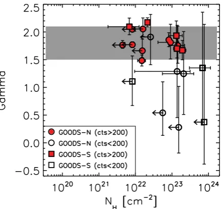
Figure 2. Photon index versus intrinsic hydrogen column density (NH)
for the X-ray-detected IR quasars in our sample, obtained using a simple absorbed power-law model (model 1); the sources XID 243N and XID 320S are not included in the plot because the andNH parameters could not
be simultaneously constrained from the spectral fit due to the low numbers of counts (<50 cts; see Section 4.1). Sources in GH-N and GH-S are rep-resented by circles and squares, respectively. Red filled symbols indicate sources with more than 200 net counts in theE=0.5–8 keV spectra; open symbols are sources with<200 net counts (i.e. with poor counting statis-tics). The grey shaded region represents the intrinsic photon indices typically found for AGN ( =1.8±0.3; e.g. Nandra & Pounds1994; Mainieri et al.
2002; Mateos et al.2005; Tozzi et al.2006). The quasars with low num-bers of counts have typically flat photon indices ( <1.5), suggesting the presence of additional spectral components, such as soft scattered emission and/or reflection (Section 4.1.1).
4.1.1 Basic spectral model fitting
We initially used a simple absorbed power-law model to character-ize the source spectra (model 1), in addition to Galactic absorption, which was fixed to the average values ofNH, Gal =1020cm−2 in GH-N andNH, Gal=9.0×1019cm−2in GH-S (Dickey & Lock-man1990). We left the photon index and the intrinsic hydrogen column density (NH) as free parameters. In Fig.2, we show the versusNHobtained from these fits. For two quasars (XID 243N and XID 320S; see Table1) with very low numbers of counts (<50 net counts, 0.5–8.0 keV), we only fit a simple power-law model with no intrinsic absorption as no useful constraints could be obtained si-multaneously on andNHfrom model 1. These two sources are not plotted in Fig.2. The results of the X-ray spectral analysis (includ-ing errors at 90 per cent confidence level) are reported in Table2. We note that 14 of the 24 analysed sources (∼58 per cent) have good counting statistics (net counts>200; see Table2). For these sources we obtained good spectral constraints with our simple model, with spectral slopes consistent with the intrinsic values typically found for AGN ( =1.8±0.3; e.g. Nandra & Pounds1994; Mainieri et al.
2002; Mateos et al.2005; Tozzi et al.2006). The sources with lower counting statistics (net counts<200) have typically flatter spectral indices, ranging between ≈0.3–1.4, with large errors. This indi-cates that the spectra of these sources are harder, and likely more obscured than those measured for the sources with higher numbers of counts; however the poor counting statistics do not allow us to simultaneously place tight constraints on the spectral parameters, andNH, as they are degenerate for low-count spectra (e.g. Mateos
et al.2008). The flat in these sources might also indicate that a simple absorbed power-law model does not properly characterize their X-ray emission and additional spectral components might be required (e.g. soft scattered component, or reflection).
For the sources with a flat photon index ( <1.5), we there-fore included an extra power-law component in the model to fit the emission at soft energies (E 1 keV; hereafter model 2). There are several processes that can cause emission at soft X-ray ener-gies, such as thermal emission from star-forming regions, radio jets, atomic processes in partially ionized gas, partial covering by a neutral absorber, or blurred ionized reflection from the inner parts of the accretion disc (e.g. Turner et al.1997; Gierli´nski & Done2004); however, given the limited numbers of counts available in our spec-tra it is not possible to fit more complex models. We therefore assume a power-law model as an approximation of the soft X-ray emission, with the photon index tied to that of the primary power law (e.g. Brightman et al.2014; Buchner et al.2014; Lanzuisi et al.
2015) to limit the number of free parameters in the model.6Fitting the spectra with model 2 constrained the power-law slopes to more typical values for AGN (see Table2), although the uncertainties on the parameters are still large. Where reasonable constraints on could not be obtained, we fixed =1.8 to obtain better constraints on the column densities. TheNHvalues resulting from the fitting of model 2 are typically higher than those obtained from model 1 and in some cases they are very high (NH>8×1023cm−2) and possibly consistent with CT absorption. In two cases (XID 435S and XID 490S; see Section 4.1.3), the column densities estimated by model 2 even exceedNH>1025cm−2. Although theseNHvalues are not reliable because the simple parametrization of the spectra with an absorbed power law is not suitable to constrain column densities of
NH>few×1023cm−2, they still indicate that these sources might indeed be heavily obscured, possibly CT. We investigate this hy-pothesis using more suitable models in Section 4.1.2. In model 2, we also estimated the fraction of intrinsic emission scattered at soft energies (fscatt), calculated from the ratio between the normaliza-tions of the scattered and intrinsic power-law components, which is on average only a few per cent, typically5 per cent (e.g. Turner et al. 1997; Ueda et al.2007). However, in some cases we find higher scattered fractions (see Table2), which might be due to the contribution from SF emission to the soft energy spectrum (E<
1–2 keV).
We also tested model 2 for sources showing significant X-ray absorption (NH>1022cm−2) from the fitting of model 1, but with steeper spectral slopes ( >1.5); the results are reported in Table2
for all of the sources where the normalization of the soft scattered power law could be constrained. Although the column densities obtained from these fits are typically higher than those obtained from model 1, the scatter on the parameters ( andNH) is larger and in all cases the results from the two models are consistent. We therefore use the best-fitting solutions from model 1 to estimate the luminosity for these sources.
From the best-fitting models (model 1 for the sources with mo1 >1.5, and model 2 for the remainders), we calculated the rest-frame 2–10 keV luminosity of the X-ray-detected IR quasars (L2−10 keV),
6We also tested the spectral fits of model 2 with a soft power-law slope free
Table 3. Spectral fits of the heavily obscured quasars using PLCABS (Yaqoob1997) and Torus (Brightman & Nandra2011).
PLCABS Torusa
No XID b N
Hc b NHc
3 171N 1.8 79.1+−5439..44 1.8 >332.5 4 190N 1.76−+00..7072 45.0+−2421..19 1.71+−00..7171 39.8+−2718..61 11 307N 1.8 43.8+−7526..90 2.39+−00..4839 >603.8d
16 423N 1.8 42.7+−23128.0.1 1.8 137.4+ 195.9
−125.6
20 149Sd 1.73+0.16
−0.16 21.9+ 4.0
−3.9 1.74+ 0.14
−0.17 19.6+ 3.2
−3.9
22 278S 1.8 84.3+−1815..78 1.8 78.1+−1816..46 23 320S 1.8 181.2+−67121.2.3 1.8 159.8+−15354.2.7 29 435S 1.90−+00..7062 685.4+−885424..20 1.90+−00..7484 251.4+−368135..69 30 490S 1.8 1013.4+−1962819.9.7 1.8 >429.5
Notes:aTo fit the Torus model, we fixed the opening angle toθ
tor=60◦
and the inclination angle toθinc=80◦, since these sources have typically
poor counting statistics and these parameters cannot be constrained from the spectral fits.bWhere sensible constraints could not be obtained simulta-neously for the photon index and the column densityNH, we fixed =
1.8.cThe column densityNHis expressed in units of 1022cm−2.dFor this
source, we did not include any soft power-law component as it is not needed in the fit.
as well as the unabsorbed 2–10 keV luminosity (L2−10 keV,intr), i.e. corrected for the best estimate of theNH(Table2).
4.1.2 Spectral models for heavily obscured AGN
From the spectral analysis using the simple models 1 and 2, for nine sources we obtained very large column density values (see Table2) indicating that they are heavily obscured (defined here as: NH>2×1023cm−2), or CT sources (NH>1.5×1024cm−2). However, simple absorbed power-law models are not suitable to reliably constrain such large column densities, as they do not ac-curately account for the Compton scattering and reflection of the absorbed photons through an optically thick material. We there-fore modelled the intrinsic emission of these sources using more appropriate models, such as: (i) PLCABS (Yaqoob 1997), which simulates the attenuation of a power-law continuum by dense, cold matter, and (ii) Torus (Brightman & Nandra2011), which is a table model based on Monte Carlo simulations of X-ray radiative transfer, self-consistently taking into account Compton scattering and iron fluorescence emission. To represent the soft X-ray emission we used a power-law model, as in model 2. To fit the PLCABS model we leftNHand free to vary, with tied to that of the soft power-law component; where both parameters cannot be constrained due to low counting statistics, we fixed =1.8. The maximum number of scatters in the model was set to 12 (see Yaqoob1997), and all other parameters were fixed to their default values. For the Torus model we fixed the inclination angle to an edge-on view,θinc=80◦, and an opening angle7ofθ
tor=60◦(see Brightman & Ueda2012). The NHand parameters were left free to vary, with tied to that of the soft scattered component, as for the PLCABS model, or fixed to
=1.8. The best-fitting parameters obtained with these two models are reported in Table3.
7We note that we also tried the fits withθ
tor=30◦, however, due to the
limited numbers of counts in the spectra it was not possible to determine which of the two geometries provided the best fit.
In general, there is good agreement between the results obtained from the PLCABS and the Torus models. Although the parameters are not tightly constrained, as the errors are relatively large, all the model solutions resulting from our analyses indicate that these quasars are, in fact, heavily obscured and in some cases, as for XID 320S, XID 435S and XID 490S, even CT. We note that three more sources, XIDs 171N, 307N and 423N are consistent with being CT quasars within the uncertainties on theNHparameter (Table3).
4.1.3 Notes on some individual sources
Although most of the source spectra can be fitted with the simple models described in the previous sections, and sensible results are obtained for their spectral parameters (see Tables2and3), some of the sources show some peculiar characteristics. Here, we describe in more detail the most interesting sources amongst our X-ray-detected IR quasar sample.
XID 171N. From the spectral fits using model 2 and PLCABS thisz=1.995 source shows a very high level of absorptionNH≈8 ×1023cm−2( =1.8), although not at CT levels. However, the residuals in the hard band (E3 keV, observed frame) suggest the presence of a reflection component and an emission line atE≈
2 keV (observed frame), typical of CT AGN spectra. Indeed, the spectral fit using the Torus model yields a column density lower limit which is well within the CT regime. Georgantopoulos et al. (2009) have also classified this source as a CT AGN. The strong emission line is consistent with the redshifted iron Kαline (E=
6.4 keV) with an equivalent width of EW=1.2+−11..61keV; given the limited counting statistics of the spectrum the uncertainties on the line EW are large, but still consistent with CT absorption.
XID 243N. The spectrum of thisz=2.004 source has only 12 net counts (0.5–8 keV) therefore a more complex model than a simple power law cannot be fit to the data. The effective photon index measured from the spectrum is =1.86+1.29
−0.87. Fitting the spectrum with an absorbed power law with =1.8 fixed to try to constrain the level of absorption results in an upper limit ofNH<8×1022cm−2, which is consistent with the source being unabsorbed. However, the X-ray luminosity of XID 243N is very low compared to the 6µm luminosity measured from its IR SED (see Table1) and the typicalLX−L6µmrelations (e.g. Lutz et al.2004; Fiore et al.2009; Mateos et al.2015). The observed X-ray luminosity is consistent with a suppression of a factor of∼300 with respect to the intrinsic luminosity measured in the MIR (see Table4), and still more than a factor of∼120 considering the intrinsic scatter of theLX−L6µm relation (∼0.35 dex; e.g. Mateos et al.2015). This suggests that XID 243N might be a heavily CT quasar (see Section 4.2 and Fig.3) and that the X-ray emission seen byChandrais only the soft scattered component (typically a few per cent of the intrinsic nuclear emission; e.g. Turner et al.1997; Ueda et al.2007; Young et al.2007, and references therein), or some emission due to SF in the host galaxy (see Table1and Section 4.3). Another possibility is that this source is intrinsically X-ray weak, as it has been found, for instance, for broad absorption line (BAL) quasars (see e.g. Luo et al.2014). However, XID 243N has never been identified as a BAL quasar to date. Although the hypothesis of intrinsically weak X-ray emission cannot be ruled out for this quasar, we favour here the heavy-obscuration interpretation (see Section 4.2).
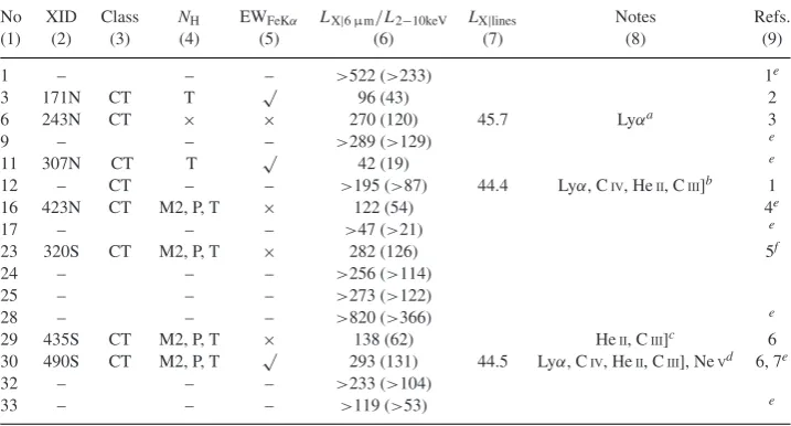
Table 4. Indication of CT quasar classification from various diagnostics for our CT quasars candidates. (1) Source number as in Table1; (2) XID as in Table1; (3) CT quasar classification: sources that we consider as secure CT quasars, based on various diagnostics explored in our analyses are marked as ‘CT’; all other sources are still CT quasar candidates; (4) X-ray spectral models yieldingNHvalues consistent, within the errors, with CT
absorptionNH>1.5×1024cm−2: ‘M2’ refers to model 2, ‘P’ to the PLCABS model and ‘T’ to the Torus model
(see Sections. 4.1.1 and 4.1.2); (5) sources showing an iron Kαline emission with EW1 keV; (6) factor of suppression of the observed X-ray luminosityL2−10keVcompared to the intrinsic X-ray luminosity derived from
the 6µm luminosity (LX|6µm) using the Lutz et al. (2004) relation; the values in parentheses correspond to the
suppression factors estimated using the lower boundary of the intrinsicLX−L6µmrelation assuming a scatter of ∼0.35 dex; (7) logarithm of the intrinsic X-ray luminosity derived from optical emission lines, in units of erg s−1;
we adopted the average emission-line flux ratios from Netzer et al. (2006) and the [OIII]λ5007-X-ray flux ratio
from Mulchaey et al. (1994); (8) list of emission lines detected in the optical spectra used to infer the intrinsic X-ray luminosity in column (7); (9) reference of previous work where these sources are classified as CT quasars, or CT quasar candidates: 1=Alexander et al. (2008), 2=Georgantopoulos et al. (2009), 3=Georgantopoulos et al. (2011b), 4=Georgantopoulos et al. (2011a); 5=Brightman et al. (2014), 6=Brightman & Ueda (2012) and 7=Feruglio et al. (2011).
No XID Class NH EWFeKα LX|6µm/L2−10keV LX|lines Notes Refs.
(1) (2) (3) (4) (5) (6) (7) (8) (9)
1 – – – >522 (>233) 1e
3 171N CT T √ 96 (43) 2
6 243N CT × × 270 (120) 45.7 Lyαa 3
9 – – – >289 (>129) e
11 307N CT T √ 42 (19) e
12 – CT – – >195 (>87) 44.4 Lyα, CIV, HeII, CIII]b 1
16 423N CT M2, P, T × 122 (54) 4e
17 – – – >47 (>21) e
23 320S CT M2, P, T × 282 (126) 5f
24 – – – >256 (>114)
25 – – – >273 (>122)
28 – – – >820 (>366) e
29 435S CT M2, P, T × 138 (62) HeII, CIII]c 6
30 490S CT M2, P, T √ 293 (131) 44.5 Lyα, CIV, HeII, CIII], NeVd 6, 7e
32 – – – >233 (>104)
33 – – – >119 (>53) e
Notes:aOptical emission line information from Adams et al. (2011);bAlexander et al. (2008);cDaddi et al. (2004); dSzokoly et al. (2004) and Feruglio et al. (2011).eThese sources also have MIR-to-optical colours typical of dust obscured galaxies (DOGs; see Fig.7and Section 5.2).fThis source is border-line CT in Brightman et al. (2014), but consistent with CT absorption within the errors, withNH=(0.5–2.9)×1024cm−2.
standard value forLX/L6µm(e.g. Lutz et al.2004; Fiore et al.2009; Mateos et al.2015), we estimate that the observed X-ray luminosity is consistent with being suppressed by a factor of∼35 (see Table4). This suppression is consistent with the effect of CT absorption, but it is less extreme than that observed for XID 243N. Moreover, no other diagnostics have been found to confirm the intrinsic AGN luminosity measured in the MIR band, therefore the possibility of intrinsic X-ray weakness cannot be ruled out.
XID 307N. In the lightly binned spectrum (1 count/bin) of this quasar, clear residuals around the observed ∼2 keV indicate the presence of a strong iron emission line, consistent with being Fe Kαat the source redshift ofz=2.14. We therefore added a Gaus-sian component to the fit, withE=6.4 keV and line width fixed atσ = 50 eV, to measure the strength of the line. Since the red-shift of this source is photometric, we initially left the redred-shift parameter in the model free to vary. From the X-ray spectral fit we obtained constraints on the redshift ofz=2.18+−00..0808, in good agreement with the photometric estimate reported in Table1. Fix-ingz=2.18 and fitting the spectrum, however, produces a very flat photon index of =0.70+0.95
−0.62, and no constraints are found on theNHparameter. Fixing =1.8 yields a column density of NH=(4.8+−38..20)×10
23cm−2with some residuals in the hard band (E
2 keV), suggesting a possible contribution from a reflection com-ponent in the spectrum. This hypothesis is supported by the high
EW measured for the iron line, EW=1.2+−10..08keV (rest frame), which is typical of CT AGN. Indeed, fitting the spectrum with the Torus model results in a column density lower limit ofNH>6× 1024cm−2(see Table3), i.e. in the CT regime. We tested this result also fitting the source spectrum with a pure reflection dominated model (i.e. PEXRAV model; Magdziarz & Zdziarski1995) with the reflection parameterR= −1 fixed, plus a Gaussian line, implying column density in excess ofNH>1025cm−2. This model provides a similarly good fit to the data as the previous models, yielding a spectral index of =2.07+0.37
−0.43. If XID 307N is really CT, its intrinsic luminosity would therefore beL2−10 keV,intr≈1045erg s−1. XID 390N. Thisz =1.146 quasar has a relatively strong iron Kαline (EW=0.38+−00..1314keV, rest frame,σ =50 eV fixed), which could be broad, as leavingσ free to vary in the fit, we obtainσ < 556 eV. Clear residuals suggest the presence of another emission line atE≈5.9 keV (rest frame) with EW≈0.28 keV, which could be a relativistically redshifted iron line from the inner parts of the SMBH accretion disc or an outflow (e.g. Fabian et al.2000). Although very interesting, more investigation on the emission lines of this quasar is beyond the scopes of this paper.
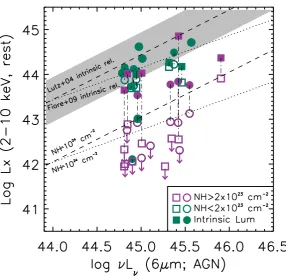
Figure 3. X-ray luminosity (2–10 keV rest frame) versus AGN rest-frame 6µm luminosity (in units of erg s−1) calculated from the SEDs; the observed
X-ray luminosity (not corrected for absorption) is plotted with open symbols, while the intrinsic luminosity, i.e. corrected for theNHmeasured from the X-ray
spectra (reported in Table2), is plotted with filled symbols. Unobscured and moderately obscured quasars (NH<2×1023cm−2) are plotted in green, while
the heavily obscured sources (NH≥2×1023cm−2) are plotted in magenta. Circles and squares correspond to sources in GH-N and GH-S, respectively. The
shaded region represents the scatter of the intrinsicLX−L6µm relation from Lutz et al. (2004) (dashed line); the dotted line represents the Fiore et al. (2009)
relation.
Although the X-ray spectrum does not show signs of any emission line, clear residuals aroundE≈1.5–2 keV (E≈5.7–7.6 keV, rest frame) indicate the presence of a strong absorption feature forming a P-Cygni type profile, which indicates the presence of a high-velocity outflow (e.g. Pounds & Reeves2009; Tombesi et al.2010). Indeed, this source has been identified in the optical band as a BAL quasar (Szokoly et al.2004). A BAL quasar interpretation would help explaining why the intrinsic X-ray luminosity of this quasar,L2−10 keV,intr≈2×1044erg s−1, which is corrected for the X-ray absorption derived from the spectral fitting, is lower than that expected from the MIR luminosityνL6µm≈8×1045erg s−1(see Fig.3), as BAL quasars have been found to be intrinsically X-ray weak (e.g. Luo et al.2014).8
XID 435S. Fitting this source spectrum with model 2 (see Section 4.1) results in a column density ofNH=(1.1−+10..27)×1025cm−2(with =1.89+−00..76), which is consistent with heavily CT material. Using the PLCABS and Torus models, we obtained smallerNHvalues of NH≈(3–7)×1024cm−2( ≈1.9), but still consistent with the source being CT (Table3). However the spectrum does not show a clear signature of a strong Fe Kαline. We note that, although these models are too complex for the limited counting statistics to provide tight constraints on the spectral parameters, the intrinsic 2–10 keV X-ray luminosity corrected for the CT column densities derived from the
8The X-ray weakness of BAL quasars is typically estimated with respect to
the optical band (αOX; e.g. Luo et al.2014). However, since BAL quasars
have SEDs consistent with those of typical quasars in the optical-to-IR bands (e.g. Gallagher et al.2007), we expect to see X-ray weakness relative to the MIR emission too.
spectral fits is in good agreement with the expectations from the MIR 6µm AGN luminosity, according to theLX−L6µmrelation. XID 435S was also classified as a CT AGN also by Brightman & Ueda (2012).
XID 490S. Thisz= 2.579 quasar shows evidence for a strong emission line, consistent with the redshifted Fe Kα line atE =
6.4 keV, with an equivalent width of EW>1 keV (although the lim-ited counting statistics prevent us from obtaining better constraints on the EW). The spectral-fitting results from model 2 constrained the intrinsic column density largely in the CT regime (see Table1). As in the previous case, fitting the spectrum with PLCABS or Torus models constrains the column density to lower values than that ob-tained from model 2 (NH≈(4–10)×1024cm−2), but still consistent with heavily CT columns. Similar results were obtained by Fer-uglio et al. (2011) and Brightman & Ueda (2012), who identified this source as CT. As for XID 435S, the intrinsic X-ray luminosity estimated by correcting for the highNHobtained from the spectral fit would place this source on theLX−L6µmrelation (see Fig.3).
4.2 Obscured AGN fraction
From the X-ray spectral analysis of the X-ray-detected sources, we found that a large fraction of the IR quasars (≈67 per cent, 16 out of 24 sources) are absorbed in the X-ray band by column densities
are consistent with being CT based on theirNH, depending on the adopted model (see Tables3and4), and on the detection of a strong iron Kαemission line (EW1 keV) in the case of XID 171N and 307N. We therefore classify these six sources as CT quasars. Due to the limited numbers of counts in the spectra, however, the strong Fe Kαline expected in CT spectra cannot be detected for all of these CT quasars.
To assess whether our IR quasars are indeed heavily obscured, or CT, we compared the X-ray luminosity (2–10 keV, rest frame) with the AGN 6µm luminosity measured from the best-fitting SEDs (see Section 3.1). Since the MIR band tends to be much less affected by obscuration than the X-ray band, the MIR luminosity is often used as a proxy for the intrinsic AGN luminosity (e.g. Lutz et al.2004; Alexander et al.2008; Gandhi et al.2009;DM13). In-deed, while unobscured sources are expected to lie on the intrinsic LX−L6µmrelation (e.g. Lutz et al.2004; Fiore et al.2009; Gandhi et al.2009; Mateos et al.2015; Stern2015), heavily obscured and CT sources, where the X-ray luminosity is strongly suppressed, are expected to have weak observed X-ray emission compared to the MIR emission, and therefore lie well below theLX−L6µm rela-tion. In Fig.3, we show the rest frameL2-10 keVversusL6µm,AGN for our IR quasars; open symbols represent the observed X-ray luminosity, while the filled symbols represent the intrinsic X-ray luminosityL2−10 keV,intr, i.e. corrected for theNHderived from the X-ray spectral fitting (see Table2). The unobscured and moder-ately obscured sources (shown in green) tend to agree with the local intrinsicLX−L6µm relation, although possibly showing a flatter slope than that defined by Lutz et al. (2004), more in agreement with Fiore et al. (2009). All of the heavily obscured IR quasars lie well below the correlation, in the region of the plot expected for CT AGN. Correcting their observed X-ray luminosity for absorption brings these sources much closer to the intrinsicLX−L6µm rela-tion, although they still lie systematically below. It is important to note that theNHof heavily obscured sources, obtained from spectral analyses ofE<10 keV data alone and with the simple parametriza-tion used here (i.e. models 1 and 2), could be underestimated, as shown in several X-ray studies of heavily obscured AGN performed usingChandraorXMM–Newtondata together with hard X-ray data (E> 10 keV) fromNuSTAR(e.g. Del Moro et al.2014; Gandhi et al.2014; Lansbury et al.2014,2015). For the three sources se-curely identified as CT quasars (XIDs 320S, 435S and 490S), the intrinsic X-ray luminosity results in very good agreement with that expected from the MIR luminosity; this is also true for XID 171N and 307N if we correct the X-ray luminosity for theNHderived from the Torus model, which gives logL2−10 keV,intr≈45.4 erg s−1 and logL2−10 keV,intr≈45.1 erg s−1, respectively, and possibly for XID 423N considering the large scatter on theNHvalue. This gives an extra indication that these sources are indeed CT.
We also note that all of the X-ray-undetected IR quasars (nine sources), for which we plot the X-ray luminosity upper limits, lie in the region of theLX−L6µmplane expected for CT sources, and therefore can be considered as CT candidates. Two of the X-ray-undetected quasars, #1 and #12, have been already investigated by Alexander et al. (2008) and were identified as CT on the basis of X-ray analyses andLX−L6µmanalyses. For #12, the intrinsic X-ray luminosity has also been estimated from the optical emis-sion lines (see Alexander et al.2008) using the average line ratio from Netzer et al. (2006) and the relation between the [OIII]λ5007 and X-ray fluxes from Mulchaey et al. (1994), yielding logLX|lines ≈44.4 erg s−1 (Table4), in agreement with that estimated from the MIR emission. This suggests that this source is intrinsically luminous, further confirming the CT nature of this quasar. The
evidence found for #12 also support our assumption that the X-ray-undetected IR quasars are CT candidates. We therefore infer that the fraction of X-ray obscured sources (NH>1022cm−2) in our sam-ple is≈76 per cent (25/33 quasars, including the X-ray-undetected quasars), with≈55 per cent being heavily obscured quasars (18/33 withNH>2×1023cm−2) and 15 out of 33 quasars (≈45 per cent) are likely to be CT.
From theLX−L6µmcomparison it also emerged that two sources having unabsorbed X-ray spectra (XID 243N and XID 287N; see Table2) have much weaker X-ray luminosity than that expected from their MIR luminosity, although for XID 287N theLX/L6µm ratio is not as extreme as for XID 243N (see Fig.3). XID 243N was classified as a candidate CT AGN also by Georgantopoulos et al. (2011b) on the basis of itsLX/L6µm ratio, similarly to our analysis. The detection of a strong Lyαemission line in the optical spectrum, which was attributed to AGN emission rather than SF by Adams et al. (2011), allowed us to estimate the expected intrinsic X-ray luminosity (as for source #12) logLX|lines ≈ 45.7 erg s−1, calculated assuming the average AGN Lyαto [OIII]λ5007line ratio from Netzer et al. (2006) and the [OIII]λ5007to X-ray flux ratio from Mulchaey et al. (1994). Although this luminosity is higher than that inferred from the MIR emission, possibly due to the uncertainties on the optical emission line ratios and perhaps to some contamination from SF emission to the Lyα flux, it supports the idea of XID 243N being intrinsically X-ray luminous; we therefore consider this source as CT (Table4). In this case, if we assume that the observed
E<8 keV spectrum is only due to scattering (∼1–3 per cent) of the intrinsic heavily obscured emission, we estimate the intrinsic X-ray luminosity to be logLX ≈ 43.6 erg s−1. This is in good agreement with the intrinsic LX−L6µm relation, supporting our classification of this quasar as CT. For XID 287N no other diagnostic has been found to establish whether this source is intrinsically X-ray luminous (and therefore likely CT) or X-ray weak (e.g. Luo et al.
2014); we thus do not include this source amongst our CT quasar candidates.
In Table4, we list all the CT quasars and CT quasar candi-dates identified in our analyses and the various indicators that point to a CT quasar classification, i.e. primarily the high column den-sity (NH>1.5×1024cm−2) and/or strong iron line (EW1 keV) derived from the X-ray spectral analysis, the suppression of the ob-served X-ray luminosity (more than a factor of∼30 for CT sources) compared to the intrinsic X-ray luminosity expected from the 6µm emission (LX|6µm), and other indicators found in the literature, such as the X-ray weakness compared to the intrinsic quasar lu-minosity derived from optical emission lines. The total fraction of CT quasars (and CT quasar candidates) in our sample is therefore
≈24–48 per cent (8–16 out of 33 quasars) and the total obscured quasar fraction is≈79 per cent.
4.3 Star formation rates