Spin-orbit alignment for three transiting hot Jupiters: WASP-103b, WASP-87b, and WASP-66b

(1)

SPIN

–

ORBIT ALIGNMENT FOR THREE TRANSITING HOT JUPITERS: WASP-103b, WASP-87b, and

WASP-66b

†

B. C. Addison1,2, C. G. Tinney1,2, D. J. Wright1,2, and D. Bayliss3

1

Exoplanetary Science Group, School of Physics, University of New South Wales, Sydney, NSW 2052, Australia;[email protected]

2

Australian Centre of Astrobiology, University of New South Wales, Sydney, NSW 2052, Australia

3

Research School of Astronomy and Astrophysics, Australian National University, Canberra, ACT 2611, Australia

Received 2015 April 6; accepted 2016 March 16; published 2016 May 18

ABSTRACT

We have measured the sky-projected spin–orbit alignments for three transiting hot Jupiters, 103b, WASP-87b, and WASP-66b, using spectroscopic measurements of the Rossiter–McLaughlin effect, with the CYCLOPS2 optical ﬁber bundle system feeding the UCLES spectrograph on the Anglo-Australian Telescope. The resulting sky-projected spin–orbit angles ofλ=3°±33°,λ=−8°±11°, andλ=−4°±22° for 103b, WASP-87b, and WASP-66b, respectively, suggest that these three planets are likely on nearly aligned orbits with respect to their host star’s spin axis. WASP-103 is a particularly interesting system as its orbital distance is only 20% larger than its host star’s Roche radius and the planet likely experiences strong tidal effects. WASP-87 and WASP-66 are hot(Teff=6450±120 K andTeff=6600±150 K, respectively)mid-F stars, making them similar to the majority of stars hosting planets on high-obliquity orbits. Moderate spin–orbit misalignments for 103b and WASP-66b are consistent with our data, but polar and retrograde orbits are not favored for these systems.

Key words:planets and satellites: dynamical evolution and stability –stars: individual(WASP-103, WASP-87, WASP-66)–techniques: radial velocities

1. INTRODUCTION

Measurements of the projected obliquity(i.e., sky-projected angle between planetary orbits and their host star’s spin axis)of exoplanetary systems are key to understanding the various mechanisms involved in the formation and migration of extrasolar planets (e.g., Albrecht et al. 2012b). As of 2015 November, 91 exoplanetary systems4, including WASP-66, WASP-87, and WASP-103 as reported here, have measured projected obliquities. These measurements have revealed a stunning diversity of planetary orbits that includes 36 planets on signiﬁcantly misaligned orbits(∣ ∣l >22 . 5 ), 15 of which are on nearly polar orbits (67 . 5 <∣ ∣l <112 . 5 or

∣ ∣l  < < 

247 . 5 292 . 5), and 9 are on retrograde orbits

(112 . 5 ∣ ∣l 247 . 5 ). The vast majority of reported spin– orbit alignments come from spectroscopic measurements of the Rossiter–McLaughlin effect (e.g., McLaughlin 1924; Rossiter

1924; Queloz et al. 2000; Ohta et al. 2005), a radial velocity anomaly produced during planetary transits from the rotation-ally broadened stellar line proﬁles of a star being asymme-trically distorted when speciﬁc regions of the stellar disk are occulted by a transiting planet.

Hot Jupiters orbiting stars cooler than 6250 K have been observed to be generally in spin–orbit alignment, while hotter stars are seen to host high-obliquity systems, as noted by Winn et al. (2010a), Albrecht et al.(2012b), and others. The reason for this observed dichotomy is thought to be linked to the amount of mass in the stellar convective envelope, which acts to tidally dampen orbital obliquities. Therefore, the realignment timescale for planets is believed to be correlated with the stellar convective envelope mass. Cooler stars have a thicker convective envelope than hotter stars (as supported by stellar

interior models; see Pinsonneault et al. 2001) and can thus drive planets that are on highly misaligned orbits onto low-obliquity orbits more quickly. Albrecht et al.(2012b)propose that the mechanism(s)responsible for migrating giant planets into short period-orbits are also randomly misaligning their orbits. Stars with Teff>6250 K can only weakly dampen orbital obliquities and are thus unable to realign planetary orbits. Therefore, the Albrecht et al. (2012b) model predicts that stars with Teff>6250 K should be observed to host planets on a random distribution of orbital obliquities while cooler stars should host planets on nearly aligned orbits.

An expansion of the parameter space for which spin–orbit angles are measured will be important for testing whether these observed trends continue to hold and so test models for orbital migration. In particular, obliquity measurements need to be carried out for suitable systems that belong to the least explored parameter space, which includes sub-Jovian, long-period, and multiplanet systems. Several mechanisms have been proposed for producing hot Jupiters and misaligning their orbits, and these can generally be grouped into two categories: disk migration and high-eccentricity migration. Disk migration occurs through the interactions between a planet and its surrounding protoplanetary disk(e.g., see Ward1997). Migra-tion through this process leads to the producMigra-tion of short-period planets on well-aligned orbits(Bate et al.2010); therefore, this mechanism is disfavored for producing the observed population of hot Jupiters on high-obliquity orbits. High-eccentricity migration through either Kozai–Lidov resonances(Kozai1962; Lidov 1962; Fabrycky & Tremaine 2007), planet–planet scatterings (Chatterjee et al. 2008), secular chaos (Wu & Lithwick 2011), or some combination of these mechanisms appears to be the likely route for producing misaligned hot Jupiters.

To further expand the sample of planets with spin–orbit alignment measurements, we have observed the Rossiter– McLaughlin effect for 66b, 87b, and

†Based on observations obtained at the Anglo-Australian Telescope, Siding

Spring, Australia.

4

This study has made use of René Heller’s Holt-Rossiter–McLaughlin

Encyclopaedia and was last updated on 2015 November. http://www.astro.

(2)

103b, three recently discovered Hot Jupiter planets from the Wide Angle Search for Planets (see Hellier et al. 2012; Anderson et al.2014; Gillon et al.2014). These systems were predicted to have large observable velocity anomalies and were good candidates for follow-up observations to determine their orbital obliquities.

WASP-103 is a late F star with a mass ofM =1.220-+0.036 0.039

M_e, a radius of R=1.436-+0.0310.052 Re, and an effective

temperature of Teff=6110160K and has a moderate rotation (vsini=10.6 0.9 km s−1) as reported by Gillon et al. (2014). It hosts a planet with a mass of MP=1.490±0.088MJ, moderately inﬂated with a radius of

= _-+

RP 1.528 0.0410.073 RJ, and an orbital period of just

= 

P 0.925542 0.000019 days(Gillon et al.2014).

WASP-103 is a particularly interesting system as it consists of a Hot Jupiter that is orbiting at only 1.2 times the Roche radius of the host star and 1.5 times its stellar diameter(Gillon et al. 2014). The planet likely experiences strong tidal forces that cause signiﬁcant mass loss with Roche-lobe overﬂow and is very near the edge of being tidally disrupted. Measuring the spin–orbit angle for this system could potentially offer insights into the processes involved in the migration of WASP-103b to its current ultra-short-period orbit. This planet currently has the second-shortest orbital period of all planetary systems with reported spin–orbit angle measurements (WASP-19b has the shortest orbital period with a measured obliquity; Hellier et al.2011; Albrecht et al.2012b; Tregloan-Reed et al.2013). WASP-87 is a mid-F star with a mass ofM_å=1.204±0.093 M_e, a radius ofR_å=1.627±0.062R_e, an effective temperature of Teff=6450±120 K, and rotating with a vsini =9.60.7 km s−1, as reported in Anderson et al. (2014). It hosts a giant planet with a mass ofMP=2.18±0.15MJ, with a

radius of RP=1.385±0.060 RJ, and an orbital period of

P=1.6827950±0.0000019 days (Anderson et al. 2014). A possible bound early-G stellar companion was observed 8. 2 from WASP-87 by Anderson et al. (2014). WASP-87 was predicted to be a good candidate for follow-up Rossiter– McLaughlin observations due to the highvsini and largeRP.

WASP-66 is a mid-F star with a mass ofM_å=1.30±0.07 M_e, a radius ofR_å=1.75±0.09R_e, an effective temperature of Teff=6600±150 K, and rotating with a vsini =13.40.9 km s−1, as reported in Hellier et al. (2012). It hosts a massive planet with a mass ofMP=2.32±0.13MJ,

slightly inﬂated with a radius ofRP=1.39±0.09RJ, and an

orbital period of P=4.086052±0.000007 days (Hellier et al. 2012). WASP-66 was also predicted to be a good candidate for follow-up Rossiter–McLaughlin observations.

2. OBSERVATIONS

We carried out the spectroscopic observations of WASP-103b, WASP-87b, and WASP-66b using the CYCLOPS2ﬁber feed with the UCLES spectrograph on the Anglo-Australian Telescope (AAT). The instrumental setup and observing strategy for the transit observations closely followed that presented in our previous Rossiter–McLaughlin publications

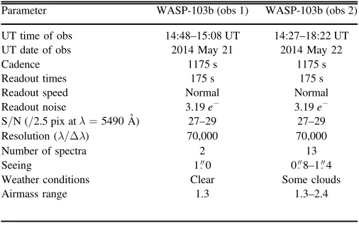
(i.e., WASP-79b and HATS-3b; Addison et al. 2013,2014a). We used a thorium–argon calibration lamp(ThAr)to illuminate all on-skyﬁbers, and a thorium–uranium–xenon lamp(ThUXe) to illuminate the simultaneous calibration ﬁber for calibrating the observations. We provide a summary of the observations in Tables 1and 2.

2.1. Spectroscopic Observations of WASP-103b

Spectroscopic transit observations of WASP-103b were obtained on the night of 2014 May 22, starting ∼50 minutes before ingress andfinishing∼15 minutes after egress. A total of 13 spectra were obtained on that night(7 during the ∼2.5 hr transit) in good observing conditions for Siding Spring Observatory with seeing between 0 7 and 1. 1 and some patchy clouds. WASP-103 was observed at an airmass of 1.3 for thefirst exposure, 1.5 near mid-transit, and 2.4 at the end of the observations. A signal-to-noise ratio (S/N)= 29 per 2.5 pixel resolution element at λ=5490Å (in total over all 16 fibers) was obtained at an airmass of 1.3, 0. 8 seeing, and integration times of 1000 s.

We also obtained two out-of-transit observations of WASP-103b on the previous night(May 21)and attempted to use them to determine the radial velocity offset between our data set and the Gillon et al.(2014)data set. Observing conditions on this night were good with seeing ~ 1. 0 and clear skies. An S/N=28 per 2.5 pixel resolution element atλ=5490Å(in total over all 16 ﬁbers) was obtained for WASP-103 when observed at an airmass of 1.3.

We observed WASP-87b on the night of 2015 February 28, starting 70 minutes before ingress and ﬁnishing 80 minutes after egress. A total of 17 spectra were obtained on that night

[image:2.612.317.570.74.243.2]

(including 9 during the ∼3 hr transit) in good observing conditions with seeing between 0 9 and 1 3. WASP-87 was

Table 1

Summary of WASP-103b Transit Spectroscopic Observations

Parameter WASP-103b(obs 1) WASP-103b(obs 2)

UT time of obs 14:48–15:08 UT 14:27–18:22 UT

UT date of obs 2014 May 21 2014 May 22

Cadence 1175 s 1175 s

Readout times 175 s 175 s

Readout speed Normal Normal

Readout noise 3.19e− 3.19e−

S/N(/2.5 pix atl=5490Å) 27–29 27–29

Resolution(λ/Δλ) 70,000 70,000

Number of spectra 2 13

Seeing 1 0 0 8–1 4

Weather conditions Clear Some clouds

Airmass range 1.3 1.3–2.4

Table 2

Summary of WASP-87b and WASP-66b Transit Spectroscopic Observations

Parameter WASP-87b WASP-66b

UT time of obs 11:03–16:44 UT 12:25–17:46 UT

UT date of obs 2015 Feb 28 2014 Mar 21

Cadence 1275 s 1375 s

Readout times 175 s 175 s

Readout speed Normal Normal

Readout noise 3.19e− 3.19e−

S/N(/2.5 pix atλ=5490Å) N/A 37–39

Resolution(λ/Δλ) 70,000 70,000

Number of spectra 17 15

Seeing 1. 0 1. 2

Weather conditions Some clouds Some clouds

(3)

observed at an airmass of 1.8 for theﬁrst exposure, 1.20 near mid-transit, and 1.1 at the end of the observations.

We obtained transit observations of WASP-66b on the night of 2014 March 21, starting ∼30 minutes before ingress and ﬁnishing∼20 minutes after egress(see Table2for a summary of these observations). A total of 15 spectra with an exposure time of 1200 s were obtained on that night (11 during the

∼4.5 hr transit)in good observing conditions with seeing∼1 2 and some patchy clouds. The airmass at which WASP-66 was observed varied from 1.0 for theﬁrst exposure, to 1.1 near mid-transit, to 2.2 at the end of the observations. An S/N=39 per 2.5 pixel resolution element atλ=5490Å(in total over all 16 ﬁbers)was obtained at an airmass of 1.0 and in 1 2 seeing.

2.4. Independent Determination of Stellar Rotational Velocity

We determined the stellar rotational velocity for WASP-103 and WASP-66 independently of the Rossiter–McLaughlin effect by fitting a rotationally broadened Gaussian to a least-squares deconvolution line profile for every spectral order(as done in Addison et al.2013,2014a)of the two best spectra of WASP-103 and WASP-66. For WASP-103, vsini =8.80.7 km s−1, and for WASP-66, vsini=11.8 0.4 km s−1.vsinidetermined from the Rossiter– McLaugh-lin effect for these two systems (as presented in Section4)is consistent with the values determined from the least-squares deconvolution method, but with significantly larger uncertain-ties.vsinias reported in Gillon et al.(2014)and Hellier et al.

(2012) for WASP-103 and WASP-66, respectively, are inconsistent with the values determined from the least-squares deconvolution method. Gillon et al.(2014)did not specify the method they used to derive the vsini value of WASP-103. Hellier et al. (2012) and Anderson et al. (2014) determined



vsini values of WASP-66 and WASP-87, respectively, by ﬁtting several unblended FeIline proﬁles.

3. ROSSITER–MCLAUGHLIN ANALYSIS

Spectroscopic data were reduced by tracing each fiber and optimally extracting each spectral order using custom MATLAB routines developed by the authors (see Addison et al.2013,2014a). For WASP-103 and WASP-66, each of the 15 useful fibers, in each of the 17 useful orders, are used to estimate a radial velocity(and associated uncertainty)by cross-correlation with a spectrum of a bright template star, HD 157347, of similar spectral type to the targets, using the IRAF task,fxcor, as described in Addison et al.(2013,2014a). For WASP-87, we found that the best radial velocities were produced by cross-correlation of each of the 15 usefulfibers in each of the 17 useful orders with a 5000 K synthetic template star. A variety of templates were trialed for cross-correlation, including observations of other bright template stars (such as HD 10700, HD 206395, and HD 86264), as well as synthetic spectra of F- and G-type stars. The lowest inter-fider5velocity scatter was obtained using the spectrum of HD 157347 for WASP-103 and WASP-66. The weighted average velocities for each observation were computed, and the uncertainties for each weighted velocity were estimated from the weighted standard

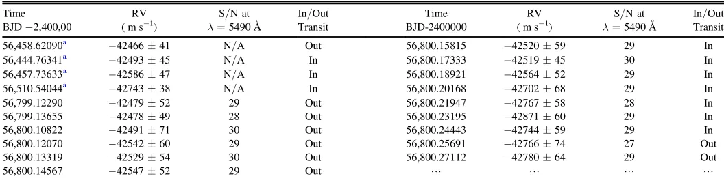
deviation of the ﬁder velocity scatter. The weighted radial velocities for the WASP-103, WASP-87, and WASP-66 transit observations, including their uncertainties and total S/N, are given in Tables3,4, and 5, respectively.

The Exoplanetary Orbital Simulation and Analysis Model

(ExOSAM; see Addison et al. 2013, 2014a) was used to determine the best-ﬁt λ and vsini values for WASP-103, WASP-87, and WASP-66 from Rossiter–McLaughlin effect measurements. We have implemented a Metropolis–Hastings Markov Chain Monte Carlo (MCMC)algorithm in ExOSAM that replaces the Monte Carlo model used in Addison et al.

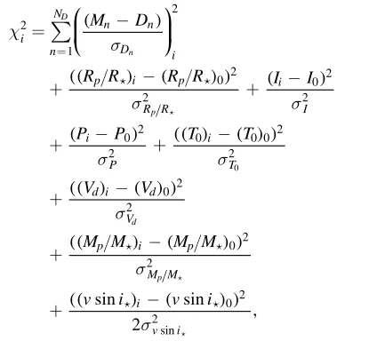
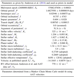
(2014a)to derive accurate posterior probability distributions of λandvsiniand to opitmize theirﬁt to the radial velocity data. Our MCMC procedure largely follows from Collier Cameron et al. (2007) and is outlined as follows. There are 16 input parameters used to model the Rossiter–McLaughlin effect for these three systems, of which 14 are prior values given by Gillon et al.(2014)for WASP-103, Anderson et al.(2014)for WASP-87, and Hellier et al. (2012) for WASP-66. The 14 priors are the planet-to-star radius ratio (R Rp ); the orbital inclination angle(I); the orbital period(P); the mid-transit time

(T0)at the epoch of observation; a radial velocity offset (Vd)

between the AAT data sets presented here and previously published data sets; a velocity offset term (Vs)accounting for

systematic effects between the AAT data sets taken over multiple nights; planet-to-star mass ratio (M Mp ); orbital eccentricity (e); argument of periastron (ϖ); two adopted quadratic limb-darkening coefﬁcients (q1 and q2); the micro-turbulence velocity (x_t); the macroturbulence velocity (vmac); and the center-of-mass velocity(VTP)at published epochTP.

Weﬁxedq1andq2,ξt,vmac, andVTPto their literature values. All three planets are also consistent with being on circular orbits, so we ﬁxed e=0 and v=0. The two out-of-transit observations obtained on 2014 May 21 for WASP-103 could not be reliably used in constrainingVdbetween our data and the

Gillon et al. (2014) data. This was due to systematic velocity offsets between the two nights that could not be well characterized from the small number of out-of-transit radial velocities that were obtained. We discarded the two observa-tions from May 21 and determined Vd using the six

out-of-transit radial velocities taken on the night of the out-of-transit. Therefore, the velocity difference,Vs, between the May 21 and

22 data sets was not used in modeling the velocity anomaly. For WASP-66 and WASP-87,Vswas not used in modeling the

velocity anomaly since the objects were observed only on one night.

We assumed Gaussian distributions for the other six priors

(R Rp ,I,P,T0,Vd, andM Mp )and allowed them to perform a random walk in the MCMC. Values for these parameters are randomly drawn from a Gaussian distribution centered on the previously accepted MCMC iteration and their reported 1σ uncertainties, as given in Tables6–8 for 103, WASP-87, and WASP-66, respectively, as described by Equations(1)– (6). The 1σ prior uncertainties remainedﬁxed in the MCMC, but are multiplied by the scale factorf, an adaptive step-size controller that evolves with the estimated uncertainties for the proposal parametersλandvsini as described below:

( ) ( )

 = - +s 

R Rp _i R Rp _i ₁ R Rp G 0, 1 ,f 1

( ) ( )

s

= - +

Ii Ii 1 IG 0, 1 ,f 2

( ) ( )

s

= - +

Pi Pi 1 PG 0, 1 ,f 3

( ) ( )

s

= - +

T0i T0i 1 T0G 0, 1 ,f 4

5

The term“ﬁder”refers to the spectrum extracted from a singleﬁber in a

(4)

( ) ( ) s

= - +

Vd i Vd i 1 VdG 0, 1 ,f 5

( ) ( )

 = - +s 

M Mp _i M Mp _i ₁ M Mp G 0, 1 ,f 6

where i is the current iteration and i−1 is the previously accepted MCMC iteration,sR Rp _ is the standard deviation on Rp/Rå, σI is the standard deviation on I, σP is the standard

deviation on P,sT0 is the standard deviation onT0,sVd is the standard deviation on Vd,sM Mp  is the standard deviation on



M Mp ,G(0, 1)is a random Gaussian deviate of mean zero and standard deviation of unity, and f is an adaptable scale factor that is used to ensure that the acceptance rate is maintained

close to the optimal value of 25%(see Tegmark et al. 2004; Collier Cameron et al.2007).

λ and vsini represent our proposal parameters for describing the Rossiter–McLaughlin effect. They perform a random walk through the parameter space that maps out the joint posterior probability distribution by the generation of a cloud of points. A value is drawn for λ and vsini at each MCMC iteration (i) by perturbing the previously accepted proposal values by a small random amount as described by Equations(7)and (8):

( ) ( )

li=li-1+slG 0, 1 ,f 7

( ) ( )

 =  - +s 

[image:4.612.41.569.74.208.2]

vsini ,i vsini ,i 1 vsini G 0, 1 ,f 8

Table 3

Radial Velocities for WASP-103(Fiber and Order Averaged)Taken on 2014 May 21 and 22

Time RV S/N at In/Out Time RV S/N at In/Out

BJD−2,400,00 (m s−1₎ _λ₌₅₄₉₀_Å _Transit _BJD-2400000 ₍_{m s}−1₎ _λ₌₅₄₉₀_Å _Transit

56,458.62090a −42466±41 N/A Out 56,800.15815 −42520±59 29 In

56,444.76341a −42493±45 N/A In 56,800.17333 −42519±45 30 In

56,457.73633a ₋₄₂₅₈₆__±_₄₇ _N_/_A _In _56,800.18921 ₋₄₂₅₆₄__±_₅₂ ₂₉ _In

56,510.54044a −42743±38 N/A In 56,800.20168 −42702±68 29 In

56,799.12290 −42479±52 29 Out 56,800.21947 −42767±58 28 In

56,799.13655 −42478±49 28 Out 56,800.23195 −42871±60 29 In

56,800.10822 −42491±71 30 Out 56,800.24443 −42744±59 29 In

56,800.12070 −42542±60 29 Out 56,800.25691 −42766±74 27 Out

56,800.13319 −42529±54 30 Out 56,800.27112 −42780±64 29 Out

56,800.14567 −42547±52 29 Out L L L L

Note.

[image:4.612.44.569.270.408.2]

a_{Published near-transit radial velocities from Gillon et al.}₍₂₀₁₄₎_{that have been adjusted for the velocity offset between the data sets.}

Table 4

Radial Velocities for WASP-87(Fiber and Order Averaged)taken on 2015 February 28

BJD−2,400,00 (m s−1) λ=5490Å Transit BJD-2400000 (m s−1) λ=5490Å Transit

56,361.75702a −13323±21 N/A Out 57,082.07871 −13416±23 N/A In

56,361.77401a ₋₁₃₃₃₂__±_₂₂ _N_/_A _In _57,082.09350 ₋₁₃₄₇₅__±_₁₅ _N_/_A _In

57,081.96030 −13315±23 N/A Out 57,082.10831 −13558±16 N/A In

57,081.97511 −13269±37 N/A Out 57,082.12311 −13561±24 N/A In

57,081.98990 −13306±29 N/A Out 57,082.13790 −13527±25 N/A In

57,082.00470 −13344±24 N/A Out 57,082.15271 −13540±18 N/A Out

57,082.01949 −13328±27 N/A In 57,082.16751 −13529±29 N/A Out

57,082.03430 −13343±22 N/A In 57,082.18230 −13507±18 N/A Out

57,082.04910 −13312±34 N/A In 57,082.19711 −13526±23 N/A Out

57,082.06391 −13362±28 N/A In L L L L

Note. a

Published near-transit radial velocities from Anderson et al.(2014)that have been adjusted for the velocity offset between the data sets.

Table 5

Radial Velocities for WASP-66(Fiber and Order Averaged)taken on 2014 March 21

BJD-2400000 (m s−1₎ _λ₌₅₄₉₀_Å _Transit _BJD-2400000 ₍_{m s}−1₎ _λ₌₅₄₉₀_Å _Transit

56,738.02316 −9967±60 39 Out 56,738.15050 −10088±53 37 In

56,738.03908 −9960±58 39 Out 56,738.16642 −10108±61 38 In

56,738.05499 −9973±58 39 In 56,738.18233 −10174±62 39 In

56,738.07090 −9991±56 38 In 56,738.19824 −10172±53 37 In

56,738.08682 −9982±63 37 In 56,738.21416 −10103±65 39 In

56,738.10273 −9925±59 38 In 56,738.23007 −10085±56 39 Out

56,738.11865 −10018±54 38 In 56,738.24599 −10051±58 39 Out

[image:4.612.44.569.470.584.2]

(5)

where σ_λ is the standard deviation on λ and svsini_ is the standard deviation onvsini.

We initially setf=0.5, but allow it to evolve in conjunction with the estimated proposal uncertainties. Following the procedure of Collier Cameron et al. (2007), we adjust f and update the uncertainties for λ and vsini from the Markov chains themselves on every 100th accepted MCMC iteration. The reason for allowing the λ and vsini uncertainties to evolve withfis to ensure that their step sizes are sufﬁcient for the adequate exploration of the parameter space. The simple linear algorithm fnew =400fold NT is used to determine f,

whereNTis the number of trailed proposals during the previous

100 successful iterations.

The best-ﬁt values and conﬁdence intervals forλandvsini are determined from calculating the joint posterior probability distribution, given as the following:

( ) ( ∣ ) ( ) ( )         l l c =

-R -R I P T V M M v i

D v i R R I P T V M M

, , , , , , , sin

, sin , , , , , ,

exp 2 , 9

p d p

0

2

where (R Rp , ,I P T V M M, 0, d, p ,l,vsini) and

( ∣ )

 Dl,vsin ,i R Rp , ,I P T V M M, 0, d, p  are the prior prob-ability distribution and the likelihood of obtaining the observed dataDgiven the modelM, respectively.χ2is calculated as

( ) (( ) ( ) ) ( ) ( ) (( ) ( ) ) (( ) ( ) ) (( ) ( ) ) (( ) ( ) ) ( )         

å

c s s s s s s s s = -+ - + -+ - + -+ -+ -+ -= ⎛ ⎝ ⎜ ⎞ ⎠ ⎟ M D

R R R R I I

P P T T

V V

M M M M

vsini vsini

2 , 10

i n

N

n n

D _i

p i p

R R i I i P i T

d i d

V

p i p

M M i v i 2 1 2 0 2 2 0 2 2 0 2 2

0 0 0 2

2 0 2 2 0 2 2 0 2 sin 2 D n p d p 0

whereiis theith accepted proposal,NDis the number of radial

velocitiesDbeingﬁtted to the modelM, andnis the nth radial velocity datum.

To determine the best-ﬁt λfor WASP-103, WASP-87, and WASP-66, we imposed a weak prior onvsini and assume a ﬂat prior onλ. This was done by setting the prior to thevsini value determined from the least-squares deconvolution method for WASP-103 and WASP-66(see Section2.4)and the value determined spectroscopically by Anderson et al. (2014) for WASP-87, using the2svsini_as the uncertainty forvsini. The decision to impose a weak prior on vsini for these three systems was based on reducing the potential bias onλfrom the large radial velocity uncertainties, inadequate sampling of the Rossiter–McLaughlin effect during their transits, and the strong correlations between λ and vsini from the small impact parameter.

The decision whether to accept or reject a given set of proposals is made by the Metropolis–Hastings rule (Collier Cameron et al.2007). This rule states that ifQiQi-1, then

the new proposal values are accepted; otherwise ifQi>Qi-1,

then the proposals are accepted with probabilityexp(-DQ 2), where D ºQ Qi-Qi-1 and Qi=c_i2. The algorithm ﬁrst converges to the optimal solution and then explores the parameter space around it.

[image:5.612.337.549.213.405.2]

The optimal solutions of λ and vsini for WASP-103, WASP-87, and WASP-66 were computed from the mean of the MCMC chains. Likewise,slandsvsini_are computed from the standard deviation of their mean. We obtained sufﬁcient convergence and well mixing of the Markov chains from 10,000 accepted MCMC iterations with no “burn-in” period.

Table 6

System Parameters for WASP-103

Parameter Value

Parameters as given by Gillon et al.(2014)and used as priors in model

Mid-transit epoch(2400000-HJD)a,T0 56800.19903±0.00075

Orbital perioda_,_P _0.925542__±__{0.000019 days}

Semimajor axisa_,_a _0.01985__±__{0.00021 AU}

Orbital inclinationa,I 86°. 3±2°. 7

Impact parametera_,_b _0.19__±__0.13

Transit deptha,(RP R)2 1.195-+0.0380.042

Orbital eccentricityb_,_e _0.0₍_assumed₎

Argument of periastronb,ϖ N/A(e=0)

Stellar reﬂex velocityb_,_K

å 271±15 m s−1

Stellar massa_,_M

å 1.220-+0.0360.039Me

Stellar radiusa,Rå 1.436-+0.0310.052Re

Planet massa,MP 1.490±0.088MJ

Planet radiusa,RP 1.528-+0.0470.073RJ

Stellar microturbulenceb_,_ξ

t 1.1±0.2 km s−1

Stellar macroturbulenceb_,_v

mac N/A

Stellar limb-darkening coefﬁcientc,q1 0.3999(adopted)

Stellar limb-darkening coefﬁcientc_,_q

2 0.2939(adopted)

Stellar effective temperatured_,_T

eff 6110±160 K(adopted)

Velocity at published epochTPb,VTP −42.001±0.005 km s

−1

RV offset between Gillon et al. and AAT data seta,Vd

32±29 m s−1

Parameters determined from a Markov Chain Monte Carlo modelﬁt using

AAT velocities

Projected obliquity anglee,λ 3 33

Projected stellar rotation velocityf,vsini 6.5±2.0 km s−1

Independent measurement ofvsini(Ind)from LSD method and Gillon et al.

(2014)vsini( )G published value

Projected stellar rotation velocity,vsini(Ind) 8.8±0.7 km s−1

Projected stellar rotation velocity,vsini( )G 10.6±0.9 km s−1

Notes. a

Prior parametersfixed to the indicated value forfinalfit, but allowed to vary in the MCMC for uncertainty estimation.

b

Parametersﬁxed at values given by Gillon et al.(2014).

c

Limb-darkening coefﬁcients determined from look-up tables in Claret &

Bloemen(2011).

d

Effective temperature from Gillon et al.(2014)and used to determine

limb-darkening coefﬁcients.

e_λ_{obtained by imposing a prior on}



vsini ofvsini(Ind)and2svsini(Ind).

f

No informative prior was imposed onvsinito obtain the best-ﬁt value and

(6)

Burn-in is a colloquial term that describes the process in which a certain number of iterations at the start of an MCMC run are discarded and the rest are kept for calculating the best-ﬁt parameters and conﬁdence intervals. Geyer in Brooks et al.

(2011, chap. 1) has suggested that this procedure is mostly unnecessary as long as the Markov chain is started reasonably close to the equilibrium distribution (determined from preliminary MCMC runs or some prior knowledge of the distribution). Therefore, we follow the advice of Geyer in Brooks et al.(2011, chap. 1)by not applying a burn-in phase in ExOSAM.

3.1. WASP-103 Results

The best-fit parameters and their 1σuncertainties for WASP-103 are given in Table6. Figure1shows the modeled Rossiter– McLaughlin anomaly with the observed velocities overplotted. The posterior probability distribution for λ and vsini resulting from our MCMC simulations is shown in Figure 2. The 1σ and 2σ confidence contours are plotted, along with normalized density functions marginalized over λand vsini with fitted Gaussians. A non-Gaussian distribution for λand



vsini is observed, suggesting that the parameters are correlated with each other or with other input parameters. λ and vsini are typically degenerate when the transit impact parameter is small(b 0.25).

The Rossiter–McLaughlin effect is seen as a positive anomaly between ∼80 minutes prior to transit and mid-transit and then as a negative anomaly between mid-mid-transit and

∼80 minutes after mid-transit. This indicates that the planetﬁrst transits across the blueshifted hemisphere during ingress and then across the redshifted hemisphere during egress, producing a nearly symmetrical velocity anomaly as shown in Figure 1. Therefore, the orbit of WASP-103b is nearly aligned with the spin axis of its host star (i.e., the system is in “spin–orbit alignment”).

A projected obliquity of l=  3 33 and a

= 

vsini 6.5 2.0 km s−1 was obtained for this system. Thevsini measured from the Rossiter–McLaughlin effect is anomalously low compared to the value determined from the least-squares deconvolution method (8.8±0.7 km s−1) and reported by Gillon et al. (2014) as 10.6±0.9 km s−1. Additional radial velocities covering the WASP-103b transit are needed in order to obtain a more precise spin–orbit angle.

We determined the best-ﬁt projected obliquity andvsinifor

WASP-87b as l= -  8 11 and

= 

vsini 9.8 0.6 km s−1(using a prior onvsini), respec-tively, as given in Table 7. The vsini measured from the Rossiter–McLaughlin effect is in agreement with the value reported by Anderson et al.(2014)of 9.6±0.7 km s−1. Figure

3 shows the modeled Rossiter–McLaughlin anomaly with the observed velocities overplotted.

This system appears to be well aligned, as shown by the nearly symmetrical velocity anomaly in Figure3, and moderate misalignments (l22 . 5 ) can be ruled out by >2σ. The Rossiter–McLaughlin effect is seen as a positive anomaly between∼100 minutes prior to mid-transit and mid-transit and then as a negative anomaly between mid-transit and ∼100 minutes after mid-transit.

The posterior probability distribution for λ and vsini resulting from our MCMC simulations is shown in Figure4. The 1σ and 2σ conﬁdence contours are plotted, along with normalized density functions marginalized overλand vsini withﬁtted Gaussians.

[image:6.612.49.291.51.243.2]

Table 8 presents the best-ﬁt parameters and their 1σ uncertainties for WASP-66. The best-ﬁt solution for λ is l= -  4 22andvsini =12.12.2 km s−1. Thevsini measured from the Rossiter–McLaughlin effect is consistent(to within the measured uncertainties)with the value reported by Hellier et al. (2012) of 13.4±0.9 km s−1 and the value we determined using the least-squares deconvolution method

Figure 1.Spectroscopic radial velocities of the WASP-103 transit. Velocities from just before, during, and after the transit are plotted as a function of time

(minutes from mid-transit at 2,456,800.19903 HJD)along with the best-ﬁtting

model and corresponding residuals. Theﬁlled blue circles with red error bars

[image:6.612.323.564.54.220.2]

are radial velocities obtained in this work on 2014 May 22. The four black circles with a cross and with blue error bars are previously published velocities by Gillon et al.(2014)using their quoted uncertainties. The zero velocity offset for the data set presented here was determined from the Gillon et al.(2014) out-of-transit radial velocities.

Figure 2.Posterior probability distribution ofλandvsinifrom the MCMC

simulation of WASP-103. The contours show the 1σand 2σconﬁdence regions

(in yellow and red, respectively). We have marginalized overλandvsiniand haveﬁt them with Gaussians(in red). This plot indicates that the distribution is somewhat non-Gaussian and suggests that there are some correlations between

(7)

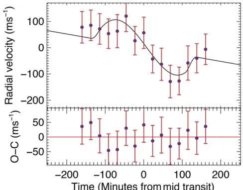
(11.8±0.4 km s−1). High-obliquity orbits can be ruled out from our data, but additional radial velocities covering the WASP-66b transit are needed to lock down a more precise spin–orbit angle. A modeled Rossiter–McLaughlin anomaly with the observed velocities overplotted is shown in Figure 5. Figure 6 shows the resulting posterior probability distribu-tion ofλandvsini, including the locations of the1sand 2σ conﬁdence contours, for WASP-66 from the MCMC simula-tions. We have also produced normalized density functions, marginalized over λandvsini and with ﬁtted Gaussians, as shown in Figure6. The resulting distribution forλandvsini appears to be Gaussian, indicating that these parameters are mostly uncorrelated.

Similar to WASP-103b and WASP-87b, the observed Rossiter–McLaughlin effect for WASP-66b is seen as a positive anomaly between ∼140 minutes prior to mid-transit and transit and then as a negative anomaly between mid-transit and ∼140 minutes after mid-transit, as shown in Figure5. This indicates that the orbit of WASP-66b is nearly aligned with the spin axis of its host star.

4. DISCUSSION

[image:7.612.320.565.51.243.2]

We have carried out measurements of the spin–orbit alignments for three hot Jupiters, WASP-103b, WASP-87b, and WASP-66b. Our results indicate that the three planets are in nearly aligned orbits with respect to the projected rotational

Table 7

Parameter Value

Parameters as given by Anderson et al.(2014)and used as priors in model

Mid-transit epoch(2400000-HJD)a,T0 57082.07656±0.00021

Semimajor axisa_,_a _0.02946__±__{0.00075 au}

Orbital inclinationa,I 81°. 07±0°. 63

Impact parametera_,_b _0.604__±__0.028

Transit deptha,(RP R)2 0.00765±0.00013

Orbital eccentricityb,e 0.0(assumed)

Argument of periastronc,ϖ N/A(e=0)

Stellar reﬂex velocityc,Kå 325±14 m s−1

Stellar massc,Må 1.204±0.093Me

Stellar radiusa,Rå 1.627±0.062Re

Planet massc,MP 2.18±0.15MJ

Planet radiusa_,_R

P 1.385±0.060RJ

Stellar micro-turbulencec_,_ξ

t 1.34±0.13 km s−1

Stellar macro-turbulencec,vmac 5.9±0.6

Stellar limb-darkening coefﬁcientd_,_q

1 0.3749(adopted)

Stellar limb-darkening coefﬁcientd,q2 0.2669(adopted)

Stellar effective temperaturee,Teff 6450±120 K(adopted)

Velocity at published epochTPc,VTP −14.1845±0.0079 km s

−1

RV offset between Anderson et al. and AAT data seta,Vd

770±12 m s−1

AAT velocities

Projected obliquity anglef_,_λ ₋₈_°__±_₁₁_°

Projected stellar rotation velocityg_, 

vsini 9.9±0.6 km s−1

Anderson et al.(2014)vsini( )A published value

Projected stellar rotation velocity,vsini( )A 12.2±1.9 km s−1

Notes. a

b

Parameterﬁxed to zero.

c

Parametersﬁxed at values given by Anderson et al.(2014).

d

Limb-darkening coefﬁcients determined from look-up tables in Claret &

Bloemen(2011).

e

Effective temperature from Anderson et al.(2014)and used to determine

f

λobtained by imposing a prior onvsiniofvsini(Ind)and2svsini(Ind).

g

[image:7.612.40.295.87.352.2]

uncertainty.

Figure 3.Spectroscopic radial velocities of the WASP-87 transit. Velocities from just before, during, and after the transit are plotted as a function of time

(minutes from mid-transit at 2,457,082.07656 HJD)along with the best-ﬁtting

model and corresponding residuals. Theﬁlled blue circles with red error bars

are radial velocities obtained in this work on 2015 February 28. The two black circles with a cross and with blue error bars are previously published velocities

by Anderson et al.(2014)using their quoted uncertainties. The zero velocity

offset for the data set presented here was determined from the Anderson et al.

(2014)out-of-transit radial velocities.

(in yellow and red, respectively). We have marginalized overλandvsiniand haveﬁt them with Gaussians(in red). The distribution appears to be Gaussian,

[image:7.612.323.563.351.519.2]

(8)

axis of their host star. The spin–orbit angle measured for WASP-103b isl=  3 33. The best-ﬁtvsini for WASP-103b using the Rossiter–McLaughlin effect and not imposing an informative prior onvsini isvsini =6.52.0 km s−1, which is in disagreement (within uncertainties) with both the value determined from the least-squares deconvolution method and the value of 10.6±0.9 km s−1reported by Gillon et al.

(2014). This is concluded to potentially be due to stellar line broadening mechanisms other than rotation.

We measured a projected obliquity of l= -  8 11 for WASP-87b. The stellar rotational velocity of WASP-87 from the Rossiter–McLaughlin effect isvsini =9.80.6 km s−1. This is in agreement (within uncertainties) with the value of

9.6±0.7 km s−1reported by Anderson et al. (2014). Out of the three systems analyzed in this work, WASP-87b has the best-constrained spin–orbit angle.

[image:8.612.321.565.51.242.2]

For WASP-66b, the spin–orbit angle is determined to be l= -  4 22. The best-ﬁt vsini obtained using the Rossiter–McLaughlin effect is vsini =12.12.2 km s−1, which is in agreement with both the value determined from least-squares deconvolution and the value of 13.4± 0.9 km s−1reported by Hellier et al.(2012). Additional radial velocities of the Rossiter–McLaughlin effect for both WASP-103 and WASP-66 are required to rule out moderately misaligned orbits; however, polar and retrograde orbits are disfavored for both systems.

Table 8

Parameter Value

Parameters as given by Hellier et al.(2012)and used as priors in model

Mid-transit epoch(2,400,000-HJD)a,T0 56738.13445±0.00035

Semimajor axisa_,_a _0.0546__±__{0.0009 au}

Orbital inclinationa,I 85 . 9  0 . 9

Impact parametera_,_b

-+

0.48 0.080.06

Transit deptha_,₍ ₎



RP R 2 0.00668±0.00016

Orbital eccentricityb,e 0.0(assumed)

Argument of periastronb_,_ϖ _N_/_A₍_e₌₀₎

Stellar reﬂex velocityb,Kå 246±11 m s−1

Stellar massb_,_M

å 1.30±0.07Me

Stellar radiusa_,_R

å 1.75±0.09Re

Planet massb,MP 2.32±0.13MJ

Planet radiusa,RP 1.39±0.09RJ

Stellar micro-turbulenceb,xt 2.2±0.3 km s−

1

Stellar macro-turbulenceb,vmac N/A

Stellar effective temperatured,Teff 6600±150 K(adopted)

Velocity at published epochTPb,VTP −10.02458±0.00013 km s−

1

RV offset between Hellier et al. and AAT data seta_,_V

d

-33-+2322 m s−1

AAT velocities

Projected obliquity anglee_,_λ _{-  }₄ ₂₂_

Projected stellar rotation velocityf,vsini 12.1±2.2 km s−1

Independent measurement ofvsini(Ind)from LSD method and Hellier et al.

(2012)vsini( )H published value

Projected stellar rotation velo-city,vsini(Ind)

11.8±0.4 km s−1

Projected stellar rotation velocity,vsini( )H 13.4±0.9 km s−1

Notes. a

b

Parametersﬁxed at values given by Hellier et al.(2012).

c

Limb-darkening coefﬁcients determined from look-up tables in Claret et al.

(2013).

d

Effective temperature from Hellier et al.(2012)and used to determine

e

λobtained by imposing a prior onvsiniofvsini(Ind)and2svsini(Ind).

f

[image:8.612.41.296.80.391.2]

uncertainty.

Figure 5.Spectroscopic radial velocities of the WASP-66 taken just before,

during, and after the transit. These are plotted as a function of time(minutes

from mid-transit at 2,456,738.13445 HJD)along with the best-ﬁtting model

and corresponding residuals. Theﬁlled blue circles with red error bars are

radial velocities obtained in this work on 2014 March 21. The zero velocity

offset for our data set was determined from the Hellier et al.(2012)

out-of-transit radial velocities(not shown). The velocities appear to be anomalously

below the best-ﬁt model of the Rossiter–McLaughlin effect during theﬁrst half of the transit. The cause for this is unknown but might be due to the planet transiting over a star spot, random noise in the data, or systematic effects that have not been accounted for in producing the radial velocities.

[image:8.612.322.564.370.536.2]

(9)

The tidal dissipation timescale was determined for WASP-103b, WASP-87b, and WASP-66b following the procedures given by Albrecht et al. (2012b). For WASP-103b, the tidal dissipation timescale is tCE=1.24´109yr (using the con-vective timescale for alignment). It is helpful to normalizetCE

to a useful stellar timescale of 5 Gyr, which results in tCE/5 Gyr=0.248. If the mass of the convective envelope is taken into account (the second approach of Albrecht et al. 2012b), the timescale becomes tmcz=3.11´106yr. Normalizing this to the model age for the host star

(Tzams=4.0´109yr)results intmcz/Tzams=7.77´10-4.

The tidal dissipation timescale for WASP-87b is tRA=1.05´1013yr (using the radiative timescale for align-ment) and tRA/5 Gyr=2.11´103. If the mass of the convective envelope is taken into consideration, then the timescale becomestmcz=1.94´1011yr andtmcz/Tzams=51

when Tzams=3.8´109yr is set to the model age of WASP-87.

For WASP-66b, the tidal dissipation timescale is tRA=1.11´1015yr (using the radiative timescale for align-ment) and tRA/5 Gyr =2.22´105. Taking the mass of the convective envelope into consideration, the timescale becomes tmcz=2.41´1012yr andtmcz/Tzams=731whenTzams=3.3

´109_{yr is set to the model age of WASP-66.}

The low-obliquity orbit found for WASP-103b is expected given the very short realignment timescale for this system. The planet is likely experiencing very strong tidal forces and could be in the process of being tidally disrupted and consumed by its host star. Investigations of the orbital migration histories of other ultra-short-period hot Jupiters through spin–orbit align-ment measurealign-ments may provide clues on the processes involved in their formation and migration, as well as tidal interactions they might be experiencing with their host star.

WASP-87 is a hot (6450±110 K), metal-poor mid-F star with a relatively long radiative realignment timescale that would not be very efﬁcient at realigning a high-obliquity planetary orbit. In addition, Anderson et al. (2014) found a nearby early-G star8. 2 from WASP-87A that appears to be a bound companion, suggesting that Kozai resonances might have inﬂuenced the obliquity of WASP-87b. Given these circumstances, WASP-87b was predicted to have high prob-ability of being misaligned, but was observed to be on a low-obliquity orbit.

Similarly, WASP-66 is a hot(Teff=6600150K), mid-F primary with a long radiative realignment timescale and was also predicted to have high probability of being misaligned. However, the orbital obliquity for this planet is low (though moderate misalignments cannot be ruled out). Orbital obliqui-ties are thought to be distributed randomly from the migration processes that produce hot Jupiters, regardless of the value of Teff(Winn et al.2010a; Albrecht et al.2012b). Therefore, the observed obliquities should be randomly distributed for systems with long tmcz and low obliquites for systems with

short tmcz (Winn et al. 2010a; Albrecht et al. 2012b).

Alternatively, WASP-66b and WASP-87b could have under-gone type 1 and 2 disk-driven migration(e.g., Lin et al.1996)

and therefore never had their orbits misaligned by the migration process.

It is important to emphasize that the true spin–orbit angle(ψ) cannot be determined directly by the Rossiter–McLaughlin effect(e.g., see Fabrycky & Winn2009). Instead, we measure the sky-projected spin–orbit angle(λ), since the orientation of

the stellar rotation axis to our line of sight is unknown. Fabrycky & Winn (2009), Morton & Johnson (2011), and Chaplin et al.(2013)have shown thatλis only a lower limit on ψand that a small∣ ∣l does not necessarily translate as a small true misalignment (∣ ∣y). However, a large∣ ∣l does indicate a large value for∣ ∣y (Fabrycky & Winn2009). There are ways of constraining the true spin–orbit angle (see, e.g., Fabrycky & Winn2009; Morton & Johnson2011; Perryman2011; Chaplin et al.2013). One way to estimate the inclination of a star’s spin axis (iå) is by combining the projected rotational velocity

(vsini from line broadening), the stellar rotational periodProt

(from high-precision photometry), and R_å (from accurate knowledge of the spectral type). Then usingsini, I, and λ, one can determineψ(see Chaplin et al.2013). Asteroseismol-ogy is a powerful technique that provides an additional means of estimating sini and determining ψ for transiting planets, independent of the Rossiter–McLaughlin effect (e.g., see Chaplin et al.2013).

Winn et al. (2010a) and Albrecht et al. (2012b) noted a dependence between the effective temperature of a host star and the degree of orbital misalignment of its planet. They observed that obliquities generally fall into two distinct populations. The coolest stars (T<6250K) tend to host planets with well-aligned orbits, while stars hotter than 6250 K host planets with a wide distribution of orbital obliquities.

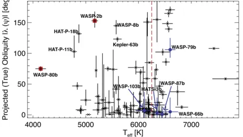
Figure7 shows an updated version of the projected orbital obliquity verses stellar temperature plot from Esposito et al.

(2014) and Addison et al. (2014a), with our measured spin– orbit angles for WASP-103b, WASP-87b, and WASP-66b and from our recently published work on WASP-79b (Addison et al.2013)and HATS-3b(Addison et al.2014a). Thisﬁgure suggests that the temperature trend observed in previous studies is no longer so clear-cut. A substantial number of stars with

<

Teff 6250K host planets on misaligned orbits. Of the 68 stars withTeff<6250K that have measured spin–orbit angles, 21

(~31%)host planets on misaligned orbits.

The most obvious outliers in Figure 7 are the six planets labeled to the left of the red dashed line at Teff=6250K, which are on signiﬁcantly misaligned orbits. These systems clearly break the observed trend between obliquity and temperature. However, two of those planets (WASP-80b, Triaud et al.2013a; and WASP-2b, Albrecht et al.2011)do not have well-constrainedλvalues despite the small uncertainties reported. For WASP-80b, this is due toλbeing almost entirely dependent on the value of vsini. For WASP-2b, Albrecht et al. (2011)could not detect the Rossiter–McLaughlin effect from the 66 spectra they obtained for this system that span the transit using the Planet Finding Spectrograph on Magellan and the High Dispersion Spectrograph on Subaru, contradicting the signiﬁcant misalignment measured by Triaud et al.(2010)from the 15 spectra they obtained using the High Accuracy Radial velocity Planet Searcher.

(10)

stars withTeff<6250K(a trend that has been noted by Winn et al.2010a; Albrecht et al.2012b; and others).

The(weakly)observed temperature trend might be explained by the thickness of the stellar convective envelope and its ability to tidally dampen orbital obliquities (as discussed in Addison et al. 2014a). Stars with Teff6250K have thin convective layers; therefore, planet–star tidal interactions are weak and unable to realign highly misaligned orbits(Albrecht et al. 2012b). In contrast, stars with Teff<6250K have a thicker convective envelope, which results in stronger planet– star tidal interactions and shorter realignment timescales. It should be noted that whileTeff=6250K is often used (e.g., Winn et al. 2010a; Albrecht et al. 2012b) as the dividing boundary between stars with thin versus thick convective layers, this boundary is only approximate. The convective zone mass actually decreases exponentially as a function of stellar temperature above Teff~5500K while decreasing linearly below this temperature(Pinsonneault et al. 2001).

Hence, the ability of a star to host planets on high-obliquity orbits for billions of years is dependent more on the tidal dissipation timescale than just the stellar effective temperature. Cool stars can host planets on misaligned orbits if the tidal dissipation timescale for realignment is very long (i.e., as suggested by the realignment timescale Equations (2)–(4) in Albrecht et al. 2012b). The relationship between tidal dissipation timescale and orbital obliquity is more clearly illustrated in Figure8, which is an updated plot6from Albrecht et al. (2013)and Addison et al.(2014a)using Equations(11)

and (12). It shows a trend toward higher orbital obliquities for

longer relative tidal dissipation timescales. This trend does appear to be more obvious than the widely reported temperature versus obliquity correlation (see Figure 7). This is likely because high obliquities are dependent on other relevant physical parameters(i.e.,a R,MP M, andMP M) than just stellar temperature alone:

( )



t = ´

-⎜ ⎟

⎛ ⎝

⎞ ⎠

q a R

1 1

10 10 yr 40 , 11

CE 9

2

6

( )  ( )

t = ´ ´ +

-⎜ ⎟

⎛ ⎝

⎞ ⎠

q q a R

1 1

0.25 5 10 yr 1 6 , 12

RA 9

2 5 6

17 2

where tCE and tRA are the tidal dissipation timescales

considering either stars with convective (Teff<6250K) or radiative (Teff 6250K)envelopes, respectively, and qis the planet-to-star mass ratio (MP M). The tidal dissipation timescalestCE and tRA in Figure 8 were derived by Albrecht

et al.(2012b)from the studies of tidal friction in close binary stars, as carried out by Zahn(1977). A potential caveat is the decision whether a star has a convective or radiative envelope. Albrecht et al. (2012b) has made the assumption that the convective envelopes for starsTeff6250K are too thin to realign orbital obliquities and therefore set the boundary at that temperature. However, this does not take into consideration the gradual thinning of the convective envelope with increasing stellar temperature.

To circumvent this issue, Albrecht et al.(2012b)devised a second approach for calculating the tidal dissipation timescales by deriving an equation that takes into account the mass of the convective envelope(tmcz; see Equation(13)):

· · ( )

t = ⎜ ⎟

⎛ ⎝ ⎞⎠

C M q R

a

1

, 13

mcz

cz 2

[image:10.612.322.563.55.192.2]

6 Figure 7.Projected orbital obliquity(λ)of exoplanets as a function of their

host star’s stellar effective temperature(Teff). We have updated thisﬁgure from

Addison et al.(2014a)to include WASP-103b, WASP-87b, and WASP-66b as

measured here, as well as the systems with newly published spin–orbit angles.

The red dashed line indicates theTeff=6250K boundary between thin and

thick stellar convective zones that inﬂuence the strength of planet–star tidal interactions that dissipate orbital obliquities. The ﬁlled blue circles represent

the systems WASP-103b, WASP-87b, WASP-66b, HATS-3b (Addison

et al.2014a), and WASP-79b(Addison et al.2013). The systems labeled to

the left of the red dashed line have anomalously large obliquities that break the observed trend of cool stars(Teff<6250K)hosting planets on low-obliquity

orbits(WASP-80b, Triaud et al.2013a; HAT-P-11b, Winn et al.2010c;

HAT-P-18b, Esposito et al. 2014; WASP-2b, Triaud et al. 2010; Kepler-63b,

Sanchis-Ojeda et al.2013; and WASP-8b, Queloz et al.2010). Theλvalues are

not well constrained for the two planets(WASP-80b, Triaud et al.2013a; and

[image:10.612.47.292.57.195.2] [image:10.612.325.571.440.499.2]

WASP-2b, Albrecht et al.2011)marked in red squares.

Figure 8. Projected spin–orbit alignments of exoplanetary systems as a function of their relative alignment timescale for stars with either convective

(CE)or radiative envelopes (RA), calibrated from binary studies. We have

updated thisﬁgure from Albrecht et al.(2013)and Addison et al.(2014a)to

include the obliquity measurements of 103b, 87b, and WASP-66b(indicated by the arrow and green dot), as well as systems with spin–orbit angles measured in the literature since these publications. Stars that have

effective temperatures higher than 6250 K are represented byﬁlled red circles

and squares with red error bars, while blueﬁlled circles and squares with blue

error bars are for stars with effective temperatures less than 6250 K. The circles and squares that are half red and blue show stars that have measured effective

temperatures consistent with 6250 K from the1suncertainty. The dark black

borders around the symbols are for systems with multiple transiting planets.

Systems with measured true obliquities (ψ) are plotted as squares, while

projected obliquities(λ)are shown as circles. WASP-79b and HATS-3b from

our previous publications(Addison et al.2013,2014a)are also shown in this

ﬁgure.

6

Figure 8 was produced from the compilation of stellar and planetary

(11)

where Mcz is the amount of mass in the convective envelope

and C is a proportionality constant equal to 105gs-1 ₍_as

provided to us by S. Albrecht 2014, private communication). Dr. Albrecht has also informed us that the equation for tmcz

(given as1 tmczµ1 Mczin Albrecht et al.2012b)is incorrect

and should be 1 tmczµMcz. This correction has been

implemented in Equation (13)and is the equation being used in this work.

We present Table9, which lists theTeff, age,λ,ψ(if known),

Mcz,tCE ortRA, andtmcz and their associated uncertainties of

the exoplanetary systems with measured spin–orbit angles,7 including WASP-66, WASP-87, and WASP-103 reported in this publication, as a reference for the community. We are not aware of any published summary of all these tidal dissipation timescales and the stellar convective zone masses. The stellar and planetary physical parameters used for calculatingMcz,tCE

or tRA, andtmcz were obtained from the TEPCat catalog8and

the Extrasolar Planets Encyclopaedia.9 Mcz were calculated

from the EZ-Web10tool made available by Richard Townsend. Results from a direct imaging survey, carried out by Ngo et al. (2015) to search for stellar companions around hot Jupiters with measured spin–orbit alignments, shows no correlation between the incidence of stellar companions and planets being on misaligned or eccentric orbits. The Ngo et al. survey targeted a sample of 50 systems, 27 hosting planets on misaligned and/or eccentric orbits, and 23 on well-aligned and circular orbits(classiﬁed as the“control sample”)to determine if any correlations exist between misaligned/eccentric hot Jupiters and the incidence of stellar companions. They discovered 19 stellar companions around 17 stars and from this result determined that the companion fraction for systems hosting misaligned planets is approximately equal (to within their reported uncertainties) to that of spin–orbit aligned systems. Their survey suggests that stellar companions may not play a dominant role in producing planets on high-obliquity orbits. Interestingly, Law et al.(2014)found tentative evidence

(at the 98% conﬁdence) for stellar companions leading to an increased rate of close-in giant planets from an adaptive optics survey of 715 Kepler planetary system candidates with the Robo-AO robotic laser adaptive optics system. Therefore, migration mechanisms that require the presence of stellar companions to operate, such as the Kozai mechanism

(Kozai 1962; Lidov 1962; Fabrycky & Tremaine 2007), are disfavored. Other migration scenarios, such as planet–planet scattering (Chatterjee et al. 2008)or primordial disk misalign-ments (from binary companions that were present at an earlier epoch but later removed through dynamical processes; see Batygin2012), might be more favored.

Our group is also conducting a similar direct imaging survey, but in the southern hemisphere, to search for stellar companions around planetary systems with measured spin– orbit alignments. We are using the Magellan Adaptive Optics system on the 6.5 m Magellan Telescope at the Las Campanas Observatory in Chile to survey nearby stars within 250 pc(see

Addison et al. 2014a, 2014b). The results from our direct imaging search will be available soon and will complement the Ngo et al.(2015)survey. Taken together, the results from the two surveys will provide a strong test of the Kozai mechanism as the dominant driver for misaligning planetary orbits.

In addition to these direct imaging searches, a radial velocity survey was conducted by Knutson et al.(2014)of 51 transiting planetary systems (50 of which were in the Ngo et al. 2015

direct imaging survey). Knutson et al. found no correlation between planets on high-obliquity orbits and the occurrence rate of long-period massive planetary companions. This seems to suggest that planet–planet scattering may also not be playing a signiﬁcant role in shaping the orbital obliquities of planets. Ngo et al.(2015)offer an alternative hypothesis, proposing that the protoplanetary disks are perturbed out of alignment at the epoch of star and planet formation due to primordially bound stellar binaries. The binary companions are later removed from the planetary systems through dynamical interactions between stars in crowded stellar clusters, eliminating their current observational signatures (Malmberg et al. 2007; Ngo et al.2015).

If high-obliquity hot Jupiters are indeed the result of primordial disk misalignments, then there should be a signiﬁcant number of debris disks observed to be in misalignment with the spin axis of their host star. Recent observations of well-aligned debris disk (e.g., Kennedy et al. 2013; Greaves et al.2014), however, argue against this mechanism being responsible for the majority of spin–orbit misalignments. This model can also be tested from measure-ments of spin–orbit alignments in coplanar multiplanet systems with stellar companions. Since multiple transiting planet systems are nearly coplanar (at least for the planets that are transiting), presumably their orbits trace the plane of the protoplanetary disk from which the planets formed originally

(Albrecht et al. 2013). Therefore, misalignments produced through dynamical mechanisms would result in planets on various orbital planes and with different observed obliquities. If these systems are found to be predominantly in spin–orbit alignment, then high-obliquity Hot Jupiter systems are likely the result of high-eccentricity migration (i.e., planet–planet scatterings, secular chaos, Kozai-Lidov resonances, etc.) instead of primordial star–disk misalignments (Albrecht et al. 2012b). If, however, the obliquities of multiplanet systems are similarly distributed to those observed for hot Jupiters, then this would suggest that spin–orbit misalignments are produced through processes other than migration such as primordial disk misalignments. Recent spin–orbit alignment measurements of transiting multiplanet systems have revealed that six host planets on low-obliquity orbits (Sanchis-Ojeda et al.2012; Albrecht et al.2013; Chaplin et al.2013; Sanchis-Ojeda et al.2015), while one hosts planets on misaligned orbits

(Huber et al. 2013). Statistical studies on the distribution of orbital obliquities of Kepler transiting planets, using the photometric stellar rotational amplitudes produced from star spots in theKeplerlight curves, suggest that planets are more likely to be found on misaligned orbits around hot stars than cool stars(Mazeh et al.2015)and if they orbit a star with only a single detected transiting planet as opposed to orbiting a star with multiple detected transiting planets (Morton & Winn 2014). The sample size, however, is too small to draw any deﬁnitive conclusions. Therefore, more multiplanet systems need to have their spin–orbit angles measured to test

7 _{Spin–orbit alignments obtained from the René Heller’s Holt-Rossiter–}

McLaughlin Encyclopaedia on 2015 November 20.http://www.astro.physik.

uni-goettingen.de/~rheller/.

8

The TEPCat catalog can be accessed athttp://www.astro.keele.ac.uk/jkt/

tepcat/tepcat.html.

9

The Extrasolar Planets Encyclopaedia can be accessed athttp://exoplanet.

eu/.

10